Key Predistribution Schemes in Distributed Wireless Sensor Network

Key Predistribution Schemes in Distributed Wireless Sensor Network using Combinatorial Designs Revisited Anupam Pattanayak, B. Majhi Computer Science & Engineering Department, National Institute of Technology, Rourkela, India – 769008 { [email protected], [email protected] }

Abstract – A Sensor Node in Wireless Sensor Network has very limited resources such as processing capability, memory capacity, battery power, and communication capability. When the communication between any two sensor nodes are required to be secured, the symmetric key cryptography technique is used for its advantage over public key cryptography in terms of requirement of less resources. Keys are predistributed to each sensor node from a set of keys called key pool before deployment of sensors nodes. Combinatorial design helps in a great way to determine the way keys are drawn from the key pool for distributing to individual sensor nodes. We study various deterministic key predistribution techniques that are based on combinatorial design. Keywords: Key predistribution, Combinatorial Design, Distributed Sensor Network

1.

Introduction

In general, a sensor node consists of four basic units: (i) Processing unit, (ii) Sensing unit, (iii) Transceiver unit, and (iv) Power unit [6]. There are a large number of sensor nodes in a sensor network. Sensor networks consisting of 10,000 nodes or 1,00,000 nodes are not uncommon. Although individual sensor nodes have limited resources, they are capable of achieving worthy task of big volume when they work as a group. Sensor networks are used in a number of different areas such as military, industry, health, environment, and home [3, 4]. Locations of sensor nodes in the network are not pre determined in most of the cases. This permits us to deploy sensor nodes in hostile environments such as border area of a hostile neighbor country by some means, for example, by using aeroplane. When secured communication between two sensor nodes is required, then they can follow either symmetric key cryptography or asymmetric key cryptography. Asymmetric key cryptography requires huge computing resources that a tiny sensor can’t afford. So a symmetric key cryptography is preferred. But key generation and distribution using Diffie-Hellman technique or public key infrastructure is also more or less infeasible in distributed sensor network consisting of resource limited sensor nodes. So distributing a set of keys to each sensor node before their deployment is a good solution. A sensor node can communicate with other node if the second one is lying within the circle of radio frequency range of the first one, and if both of them share a common key. In a key predistribution scheme, there are three phases. These are key predistribution,

shared-key discovery, and path-key establishment [9]. In key predistribution phase a set of keys are chosen from a key pool following a predetermined order. In shared-key discovery phase if two nodes want to communicate and they are lying in one another’s radio frequency range then they communicate to each other and find which one is the common key between them. If two nodes Ni and Nj want to communicate with each other and there is no common key then they look for one or more intermediate nodes such that every pair of adjacent nodes share a common key, so that Ni and Nj are able to communicate with each other securely. This phase is known as path-key establishment. In our survey we focus on the key predistribution phase only. The first work related to key predistribution can be traced back in 1985, by R. Blom [16]. The research momentum in this field gained after the seminal work by Eschenauer & Gligor [17]. Keys of a key-chain are selected from a key pool randomly and assigned to a sensor node. This method of key predistribution is probabilistic. Key predistribution schemes based on combinatorial designs are deterministic. Our main focus is to present key predistribution schemes based on combinatorial designs only. We have also given examples of way of key generations by the different schemes, whenever possible. We believe this will particularly help the new researchers in this field. For a very good discussion on the applicability of combinatorial designs in key predistribution one can refer the work by K M Martin [18]. We have organized this survey paper as follows. In section 2, we have discussed necessary background in combinatorial design. In section 3 we have mentioned the various metrics to judge a key predistribution scheme (KPS). Then in section 4 we have discussed the KPS based on projective plane and KPS based on generalized quadrangle. Transversal design based KPS is discussed in section 5. PBIBD based KPS has been discussed in section 6. Section 7 describes the KPS based on orthogonal array. Section 8 discusses the KPS based on 3-design, followed by conclusion in section 9. 2.

Background

The subject combinatorial design found its application initially in the design of experiments in statistics for long days. Then it was used extensively in the field of coding theory. Also combinatorial design techniques have been used in numerous other area of computer science such as Boolean function, authentication code, visual cryptography, multiple accesses to channel, software testing etc. For detail on these areas where combinatorial designs have been used, one can refer [2]. In this paper we will discuss the works done on key predistribution schemes that are devised following different combinatorial design techniques. 2.1

Combinatorial Design

Combinatorial design theory is interested in arranging elements of a finite set into subsets to satisfy certain properties. It is the study of families of subsets with various prescribed regularity properties. Members of the universal set S in a combinatorial design

are usually called treatments, or varieties, and the subsets chosen are called blocks. A regular design based on a v-set S is a collection of k-sets from S such that every member of S belongs to r of the k-set blocks. It is usual to write b for the number of blocks in a design. So a regular design has four parameters: v, b, r, and k. However these parameters are not independent. A regular design is represented as (v, b, r, k)-design. In any regular design, b*k = v*r. A block design is proper if all of its block have same length. The number of blocks that contain a given treatment is the replication number, r. If all v treatments occur in a block of a design, then the block is called complete. If a regular design has the property this property then that design is called complete design. Complete design is of very little interest unless some further structure is imposed (such as in Latin Square). In a design, if at least one block is incomplete then that design is an incomplete design. If v = b, the design is called symmetric. If x and y are any two different treatments in an incomplete design, we shall refer to the number of blocks that contain both x and y as the covalency of x and y, and write it as λxy. 2.2

BIBD

A Balanced Incomplete Block Design (BIBD) is an arrangement of v distinct objects into b blocks such that each block contains exactly k distinct objects, each object occurs in exactly r different blocks, and every pair of distinct objects occurs together in exactly λ blocks. The design can be expressed as (v, k ,  ) , or equivalently (v, b, r , k ,  ) , where:  (v  1)  r (k  1) and bk  vr . Following is an example of (9,12,4,3,1)-BIBD: 123 456 789 147 258 369 168 249 357 159 267 348 A BIBD is symmetric BIBD when b=v and therefore r=k. It is represented as (v, k, λ)-design. For every prime power q ≥ 2, there exists a symmetric design (q2+q+1, q+1, 1). 2.3

Projective Plane

A Projective Plane consists of a set of lines and a set of points, and a relation between points and lines called incidence, having the following properties: 1. Given any two distinct points, there is exactly one line incident with both of them. 2. Given any two distinct lines, there is exactly one point incident with both of them. 3. Every point has q+1 lines through it. 4. Every line contains q+1 points. A projective plane is therefore a symmetric (q2 + q + 1, q+1, 1) block design. A projective space PG(d, q) of dimension d over a field F is constructed from the vector space of dimension d+1 over F as follows [7]: 1. Objects are all subspaces of the vector space, 2. Two objects are incident if one contains the other, Subspaces with dimension 1, 2, and d are called points, lines, and hyperplanes respectively. A partial linear space arranges objects into subspaces in the form of incidence structure. These subsets are called lines. In a partial linear space [7]: 1. Each line is incident with at least two points, and 2. Any two points are incident with at most one line. A partial geometry [7] is a partial linear space where: 1. Number of points on a line is constant, 2. Number of lines through a point is constant, and 3. Given a point x on a line L, the number of points on L that are collinear with x is constant. Finite generalized quadrangle (GQ) is a special class of partial geometry. 2.3

Transversal Design

A Group-divisible design of type gu and block sizek is a triplet (X, H, A), where X is a finite set of cardinality gu, H is a partition of X into u parts (called groups) of size g, and A is a set of subsets of X (called blocks), that satisfy following properties: 1) H1  A1  1 for H1  H and every A1  A. 2) Each pair of elements of X from different groups occurs in exactly one block in A. A transversal design (TD) is a group-divisible design. A TD(k, n) is equivalent to a set of k-2 mutually orthogonal latin squares of order n. A (v, b, r, k)-configuration is a (v, b, r, k)-1 design such that the number of common point between any two blocks is either zero or one. A (v, b, r, k, λ)-BIBD is a (v, b, r, k)-1 design such that any pair of points occur in exactly λ blocks. 2.4

PBIBD

An association scheme with m associate classes on the set X is a family of m symmetric anti-reflexive binary relations on X such that:

1. any two distinct elements of X are i-th associates for exactly one value of i, where 1≤i≤m, 2. each element of X has ni i-th associates, 1≤i≤m, and 3. for each i, if x and y are i associates, then there are pijl elements of X which are both j-th associates of x and l-associates of y. The numbers vi (1≤i≤m) and pijl (1≤i,j,l≤m) are called the parameters of the association schemes. A triangular association scheme is a partially balanced design with two associate classes. Here the association scheme is an array of n rows and n columns, and number of varieties is n(n-1)/2. It has the following properties: 1. The principal diagonal elements (from top-left to bottom-right) are left blank. 2. The n(n-1)/2 positions above the principal diagonal are filled with numbers 1, 2, …, n(n-1)/2 corresponding to the varieties. 3. The n(n-1)/2 positions elements below the diagonal are filled in a way such that the array is symmetrical. 4. For any variety i, the first associates are those elements which lie in the same row (or the same column) as i, the second associates are the rest of the elements. A partially balanced incomplete block design with m associate classes, denoted by PBIBD(m) is a design on a v-set X, with b blocks each of size k and with each element of X being repeated r times, such that if there is an association scheme with m classes defined on X where, two elements x and y are ii-th (1≤i≤m) associates, then they occur together in λi blocks. Such design is denoted by PB[k, λ1, λ2, … , λm; v]. 2.5

Orthogonal Array

An N x K array A with elements from S (|S|=s) is said to be OA with s levels, strength t and index λ (0≤t ≤k) if every N x t sub-array of A contains each t-tuple based on S exactly λ times as a row. When λ=1 we say OA has index unity. N, k, s, t, λ are parameters of OA. λ can be derived from other parameters (λ=N/st). So an OA is represented as OA(N, k, s, t). 2.5

t-design

A t-design is a design (X, A) such that the following properties are satisfied: (1) |X| = v, (2) each block contains exactly k points, and (3) every set of t distinct points is contained in exactly λ blocks. The general term t-design is used to denote any t-(v, k, λ)-design. A 2-(v, k, λ)-design is just a (v, k, λ)-BIBID. 3.

Metrics of key predistribution Scheme

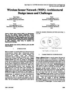
Metrics to judge a given key predistribution scheme are: connectivity, resiliency, scalability, complexity of shared-key discovery and path-key establishment. Given any two nodes, connectivity defines the probability that there is a common key between them. Resiliency refers to the sustainability of the sensor network when some of its nodes have compromised by attacker. There are two kinds of resiliency: E(s), and V(s). Given a sensor network, if s nodes are compromised, then E(s) = number of communication links broken / total number of communication links, V(s) = number of victim nodes / total number of nodes. Scalability means given the same key pool and same key-chain length the ability to add new nodes in the distributed sensor network and assign them key-chains. Complexity of shared key discovery refers to the number of computation steps needed to find out the common key between any two sensor nodes. Complexity of path-key establishment refers to the number of computations needed to find common keys between adjacent intermediate nodes when there is no common key between two sensor nodes. We illustrate connectivity and resiliency using the example given below.

Figure 3.1 A sensor network of six sensor nodes. In the above network there are six sensor nodes. The key pool is {1, 2, 3, 4}. Each sensor has two keys. We assume all these sensors are in the communication range of each other. So any two nodes in this network can communicate if they have a common key. For example, Node 3 and Node 4 share a common key 1. So there is a communication link between them. But nodes 4 and 5 do not share any key, so there is no communication link between them. In the above example, there are 6 nodes. So maximum number of connections possible in the network is

= 15. The number of direct communication

links that exist in the network is 11. So connection probability p =

= 0.733.

In our example, let us suppose that s = 2 and attacker has captured the nodes 1 and 2. So she is able to extract the keys used by these nodes. This compromised key pool set is {1, 2, 4}. As a result we can check that among eleven communication links total nine communication links are compromised. So E(2) = = 0.818. And we see that due to this compromise of nodes 1 and 2, a different node that is node 4 is no more able to

communicate with no other node. Because all keys of this node are compromised. In other words this node 4 has become victim node due to the compromise of nodes 1 and 2. Note that no other node turns victim node. So here V(2) = = 0.066. 4.

KPS based on Projective Plane, and Generalized Quadrangle

Now we will discuss combinatorial design based key predistribution schemes (KPS). We’ll first discuss KPS proposed by Camtepe and Yener. This was the first such proposal that uses combinatorial design for key predistribution in wireless sensor network. They have used two kinds of designs – projective plane and generalized quadrangle. Next we’ll discuss KPS proposed by Lee and Stinson. They have used transversal design for KPS. Dong, Pei, and Wang. They have proposed two different kind of KPS based on Orthogonal Array, and based on 3-design. At last we’ll see the KPS, proposed by Ruj and Roy, which is based on partially balanced incomplete block design (PBIBD). 4.1

KPS based on Projective Plane

To construct (q2+q+1, q+1, 1) symmetric design, Camtepe and Yener have used complete set of (q-1) mutually orthogonal latin squares (MOLS) [7]. A Latin Square on q symbols is a q x q array such that each symbol appears only once in each row and in each column. Order of a latin square is q. Suppose A = (aij), and B = (bij) are two q x q latin squares. These two squares are orthogonal if the superimposition of two squares produces a square with all distinct elements. Latin squares A1, A2, A3, … , An are mutually orthogonal latin squares (MOLS) if they are orthogonal in pairs. A set of (q-1) MOLS of order q is called complete set, where q is a prime power. A complete set of (q-1) MOLS can be used to construct affine plane of order q, which is a (q2, q, 1) design. An Affine plane of order q can be transformed to a projective plane of order q, which is a (q2+q+1, q+1, 1) symmetric design. 4.1.1 Algorithm for constructing a (q2+q+1, q+1, 1) symmetric design Input: total number of sensor nodes, N Step 1. Find the minimum prime power q that satisfies q2+q+1 ≥ N. Step 2. Construct q-1 MOLS of order q. Step 3. Construct q2 blocks of affine plane of order q. Step 4. This affine plane is basically projective plane, which can be used for key predistribution. Each block of this design is assigned to a sensor node as its key-chain.

4.1.2 Simpler Construction Method Ruj and Roy used an equivalent but simpler construction method in [11] based on the technique given in [12]. Blocks (or sensor nodes) are indexed by the identifiers (1, b, c), (0, 1, c), and (0, 0, 1) where b, c  GF(q). So there will be total q2+q+1 blocks.

Elements (or keys) are indexed by (x, y, z) where x, y, z  GF(q). The identifiers of these nodes are either (x, y, 1), (x, 1, 0), (1, 0, 0) where x, y, z  GF(q). So there are total q2+q+1 keys. And these keys are distributed among q2+q+1 number of nodes according to the following rule: A key (x, y, z) is distributed to node (a, b, c) if ax + by + cz = 0 mod q. This design yields PG(2, q). We now give the algorithm to predistribute keys in PG(2, q) following [11]. Step1. For all b  q do Step 2. For all c  q do Step 3. For all y  q do Step 4. x = -(c + by) mod q. Step 5. Assign key (x, y, 1) to node (1, b, c) Step 6. [ end of step 3 loop] Step 7. Assign key (-b, 1, 0) to node (1, b, c) Step 8. [ end of step 2 loop] Step 9. [ end of step 1 loop] Step 10. For all c  q do Step 11. For all x  q do Step 12. Assign key (x, -c, 1) to node (0, 1, c) Step 13. [ end of step 11 loop] Step 14. Assign key (1, 0, 0) to node (0, 1, c) Step 15. [ end of step 10 loop] Step 16. For all x  q do Step 17. Assign key (x, 1, 0) to node (0, 0, 1) Step 18. [ end of step 11 loop] Step 19. Assign key (1, 0, 0) to node (0, 0, 1) Algorithm 1. Key predistribution using PG(2, q) Suppose we need to assign key-chains to a distributed wireless sensor network consisting of 21 nodes following the above describe key predistribution algorithm. So we take q = 4 as q2+q+1 = 21. The following table shows the nodes and their assigned keys following the above scheme in PG(2, q). Node Index (1,0,0) (1,0,1) (1,0,2) (1,0,3) (1,1,0) (1,1,1) (1,1,2) (1,1,3) (1,2,0) (1,2,1)

(0,0,1) (3,0,1) (2,0,1) (1,0,1) (0,0,1) (3,0,1) (2,0,1) (1,0,1) (0,0,1) (3,0,1)

(0,1,1) (3,1,1) (2,1,1) (1,1,1) (3,1,1) (2,1,1) (1,1,1) (0,1,1) (2,1,1) (1,1,1)

Keys (0,2,1) (3,2,1) (2,2,1) (1,2,1) (2,2,1) (1,2,1) (0,2,1) (3,2,1) (0,2,1) (3,2,1)

(0,3,1) (3,3,1) (2,3,1) (1,3,1) (1,3,1) (0,3,1) (3,3,1) (2,3,1) (2,3,1) (1,3,1)

(0,1,0) (0,1,0) (0,1,0) (0,1,0) (3,1,0) (3,1,0) (3,1,0) (3,1,0) (2,1,0) (2,1,0)

(1,2,2) (1,2,3) (1,3,0) (1,3,1) (1,3,2) (1,3,3) (0,1,0) (0,1,1) (0,1,2) (0,1,3) (0,0,1)

(2,0,1) (1,0,1) (0,0,1) (3,0,1) (2,0,1) (1,0,1) (0,0,1) (0,3,1) (0,2,1) (0,1,1) (0,1,0)

(0,1,1) (3,1,1) (1,1,1) (0,1,1) (3,1,1) (2,1,1) (1,0,1) (1,3,1) (1,2,1) (1,1,1) (1,1,0)

(2,2,1) (1,2,1) (2,2,1) (1,2,1) (0,2,1) (3,2,1) (2,0,1) (2,3,1) (2,2,1) (2,1,1) (2,1,0)

(0,3,1) (3,3,1) (3,3,1) (2,3,1) (1,3,1) (0,3,1) (3,0,1) (3,3,1) (3,2,1) (3,1,1) (3,1,0)

(2,1,0) (2,1,0) (1,1,0) (1,1,0) (1,1,0) (1,1,0) (1,0,0) (1,0,0) (1,0,0) (1,0,0) (1,0,0)

Table 4.1 Distribution of keys following KPS using PG(2, q). 4.1.2

Analysis of projective plane based KPS

In projective plane any two blocks share a common element. So when we assign each block to a sensor node, we can say that a node always shares a common key with any other node, and this number of common key is always one. This is a very good property. So connective probability = 1 here. But when the network size is large, then each node requires quite large memory because the number of keys in a node is near equal to the √N, where N is the number of nodes in the network. This design is not scalable. Given a fixed key-chain size k=q+1, this design can support a sensor network of size N ≤ q2+q+1. To accommodate more sensor nodes we have to raise the value of k to the next prime power. 4.2

KPS based on Generalized Quadrangle

Camtepe and Yener also proposed another KPS based on generalized quadrangle. In a GQ(s, t), there are v = (s+1)(t+1) points and b = (t+1)(st+1) lines. Each line contains s+1 points, and each point appears on t+1 lines. So a line shares a point with t(s+1) other lines. If we look from key predistribution, it can be rephrased as a block shares a key with t(s+1) other blocks. If two blocks do not share a key, there are s+1 other blocks sharing a key with both of those two blocks. 4.2.1 Three known generalized quadrangles GQ(q, q), GQ(q, q2), and GQ(q2, q3) have been used. A point is a vector X = in GF(q) for PG(d, q) and in GF(q2) for PG(d, q2). GQ(q, q) is from projective space PG(4, q) with canonical equation: Q( X ) = x 02 + x1x2 + x3x4 = 0. GQ(q, q2) is from PG(5, q) with canonical equation:

Q( X ) = f(x0, x1) + x2x3 + x4x5 = 0 where f(x0, x1) is an irreducible binary quadratic of the form f(x0, x1) = c x 02 + x0x1 + x 12 . GQ(q2, q3 ) is from PG(4, q2) with canonical equation: Q( X ) = f(x0, x1) + x2x3 + x4x5 = 0 where f(x0, x1) is an irreducible binary quadratic of the form f(x0, x1) = x q0 1 + x 1q 1 + x q2 1 + x 3q 1 + x q4 1 = 0. A point a = is in the projective space PG(d, s) with the canonical equation Q( X ) = 0 if Q( a )=0. Points a and b are said to be collinear if B(a, b) = 0 c = . where B(a, b) = Q( c ) – Q( a ) – Q( b ) for

4.2.2 Construction of GQ(s, t) based KPS Input: GQ(s,t), and total number of sensor nodes N. Step 1. Take the minimum prime power q such that number of blocks in design, b ≥ N. Step 2. Find v = (s + 1)(st + 1) points holding the corresponding canonical equation. Step 3. For every point a , generate the set of points collinear with a . Step 4. Construct b = (t + 1)(st + 1) lines with s+1 points. For example take the generalized quadrangle GQ(q, q) where q=2. So from this GQ we can obtain (q+1)(q2+1)=15 points such that each point x = satisfies the canonical equation Q( x ) = x 02 + x1x2 + x3x4 = 0. Among those points we select (q+1)( q2+1)=15 points that satisfy this canonical equation. This operation is in GF(2). Since GQ(q, q) is from PG(4, q). So there will be four elements in each point vector. For example, we choose the following points in GQ(2, 2): Point Id 0 1 2 3 4 5 6 7 8 9 10 11 12

Points

13 14 Figure 4.1 Points in GQ(2, 2) Points a and b are said to be collinear (which is denoted by a  b ) if [Q( c ) – Q( a )-Q( b )]=0, where c =< a0+ b0, a1+ b1, … , ad+ bd >. Let a  represents the set of points collinear with point a . Then a line connecting two distinct and collinear points a and b is denoted by a   b  . 4.2.3 Example of KPS using Generalized Quadrangle Suppose, a = , b = , a  = {1, 3, 4, 6, 7, 9, 10, 11, 12}, b  = {0, 1, 8, 10, 11}. So a   b  = {1, 10, 11} that contains q+1=3 points. So this line represented by a   b  is a block or equivalently a key-chain in key predistribution scheme. Following is the example given in [7] we list the blocks obtained from GQ(2, 2): The key pool set, v = {0, 1, 2, 3, 4, 5, 6, 7, 8, 9, 10, 11, 12, 13, 14}, and the blocks are {0, 7, 8}, {0, 11, 12}, {0, 3, 4}, {2, 11, 14}, {1, 7, 9}, {1, 11, 13}, {1, 3, 5}, {4, 10, 13}, {2, 3, 6}, {5, 10, 12}, {4, 9, 14}, {2, 7, 10}, {6, 8, 13}, {6, 9, 12}, {5, 8, 14}. 4.2.4 Analysis of KPS based on Generalized Quadrangle Probability that two blocks share a key is t (s  1) PGQ = ( t  1)(st  1) GQ(s, t) provides better resilience than projective plane [7].

5.

Key Predistribution Scheme using Transversal Design

This scheme is proposed by Lee and Stinson [9]. This scheme uses Transversal design, which is a special kind of group-divisible design. Here, any two distinct blocks intersect in zero or one point. 5.1

Algorithm To Derive TD(t, p) We write the algorithm to construct transversal design as given in [9]. Step 1. Define X = { 0, 1, … , k-1} x p. Step 2. For 0 ≤ x ≤ k-1, define Hx = { x } x p. Step 3. Define = { Hx | 0 ≤ x ≤ k-1 }. Step 4. For every ordered pair (i, j)  p x p,

define a block Ai,j = { (x, ix+j mod q) | 0 ≤ x ≤ k-1 }. Step 5. Obtain A = { Ai,j | (i, j)  p x p}. Step 6. (X, , A) is a TD(k, p). 5.2

Example of Transversal Design based KPS

To understand the above algorithm, we give the following example showing how do the blocks are formed. In this example number of blocks = 49, block size = 4, a prime power = 7. Now the blocks are constructed as below:

A0, 0:

(0, 0), (1, 0), (2, 0), (3, 0)

A0, 1:

(0, 1), (1, 1), (2, 1), (3, 1)

A0, 2:

(0, 2), (1, 2), (2, 2), (3, 2)

A0, 3:

(0, 3), (1, 3), (2, 3), (3, 3)

A0, 4:

(0, 4), (1, 4), (2, 4), (3, 4)

A0, 5:

(0, 5), (1, 5), (2, 5), (3, 5)

A0, 6:

(0, 6), (1, 6), (2, 6), (3, 6)

A1, 0:

(0, 0), (1, 1), (2, 2), (3, 3)

A1, 1:

(0, 1), (1, 2), (2, 3), (3, 4)

A1, 2:

(0, 2), (1, 3), (2, 4), (3, 5)

A1, 3:

(0, 3), (1, 4), (2, 5), (3, 6)

A1, 4:

(0, 4), (1, 5), (2, 6), (3, 0)

A1, 5:

(0, 5), (1, 6), (2, 0), (3, 1)

A1, 6:

(0, 6), (1, 0), (2, 1), (3, 2)

A2, 0:

(0, 0), (1, 2), (2, 4), (3, 6)

A2, 1:

(0, 1), (1, 3), (2, 5), (3, 0)

A2, 2:

(0, 2), (1, 4), (2, 6), (3, 1)

A2, 3:

(0, 3), (1, 5), (2, 0), (3, 2)

A2, 4:

(0, 4), (1, 6), (2, 1), (3, 3)

A2, 5:

(0, 5), (1, 0), (2, 2), (3, 4)

A2, 6:

(0, 6), (1, 1), (2, 3), (3, 5)

A3, 0:

(0, 0), (1, 3), (2, 6), (3, 2)

A3, 1:

(0, 1), (1, 4), (2, 0), (3, 3)

A3, 2:

(0, 2), (1, 5), (2, 1), (3, 4)

A3, 3:

(0, 3), (1, 6), (2, 2), (3, 5)

A3, 4:

(0, 4), (1, 0), (2, 3), (3, 6)

A3, 5:

(0, 5), (1, 1), (2, 4), (3, 0)

A3, 6:

(0, 6), (1, 2), (2, 5), (3, 1)

A4, 0:

(0, 0), (1, 4), (2, 1), (3, 5)

A4, 1:

(0, 1), (1, 5), (2, 2), (3, 6)

A4, 2:

(0, 2), (1, 6), (2, 3), (3, 0)

A4, 3:

(0, 3), (1, 0), (2, 4), (3, 1)

A4, 4:

(0, 4), (1, 1), (2, 5), (3, 2)

A4, 5:

(0, 5), (1, 2), (2, 6), (3, 3)

A4, 6:

(0, 6), (1, 3), (2, 0), (3, 4)

A5, 0:

(0, 0), (1, 5), (2, 3), (3, 1)

A5,1:

(0, 1), (1, 6), (2, 4), (3, 2)

A5, 2:

(0, 2), (1, 0), (2, 5), (3, 3)

A5, 3:

(0, 3), (1, 1), (2, 6), (3, 4)

A5, 4:

(0, 4), (1, 2), (2, 0), (3, 5)

A5, 5:

(0, 5), (1, 3), (2, 1), (3, 6)

A5, 6:

(0, 6), (1, 4), (2, 2), (3, 0)

A6, 0:

(0, 0), (1, 6), (2, 5), (3, 4)

A6,1:

(0, 1), (1, 0), (2, 6), (3, 5)

A6, 2:

(0, 2), (1, 1), (2, 0), (3, 6)

A6, 3:

(0, 3), (1, 2), (2, 1), (3, 0)

A6, 4:

(0, 4), (1, 3), (2, 2), (3, 1)

A6, 5:

(0, 5), (1, 4), (2, 3), (3, 2)

A6, 6:

(0, 6), (1, 5), (2, 4), (3, 3)

5.3 -Common Intersection Designs (-CID) Suppose that two nodes Ni and Nj are located within each other’s communication range, but do not share a common key. So we look for a common neighbor Nh that shares a common key with both Ni and Nj. Suppose (X, A) is a (v, b, r, k)-configuration. (X, A) is a -CID provided that

A

h



 A A i  A h   and A j  A h    

Whenever Ai  Aj = .

It is always preferable to construct a (v, b, r, k)-configuration with  as high as possible. This maximum  is denoted as *(v, b, r, k).

5.4

Analysis of KPS based on Transversal Design

Let (v, b, r, k)-configuration, which is a -CID, is used for KPS. Suppose Ni and Nj are two nodes located within each other’s communication range. The probability that Ni and Nj share a common key is k * (r  1) . b 1 If the number of nodes, compromised by attacker, is s then resiliency V(s) is as follows:

P=

V(s) = 1 –

6. PBIBD based KPS Ruj and Roy have used PBIBD with two associate classes based on triangular association scheme [10]. Let us take the following example:

* 1 A= 2 3 4

1 * 5 6 7

2 5 * 8 9

3 4 6 7 8 9 * 10 10 *

In this design, v = b = 10, r = k = 6. The blocks that are formed from this design are as follows: {2, 3, 4, 5, 6, 7}, {1, 3, 4, 5, 8, 9}, {1, 2, 4, 6, 8, 10}, {1, 2, 3, 7, 9, 10}, {1, 2, 6, 7, 8, 9}, {1, 3, 5, 7, 8, 10}, {1, 4, 5, 6, 9, 10}, {2, 3, 5, 6, 9, 10}, {2, 4, 5, 7, 8, 10}, {3, 4, 6, 7, 8, 9}. So if we map this to a sensor networks the key-chain corresponding to nodes are as follows: Nodes Block 0 Block 1 Block 2 Block 3 Block 4 Block 5 Block 6 Block 7 Block 8 Block 9

Key-Chain {2, 3, 4, 5, 6, 7} {1, 3, 4, 5, 8, 9} {1, 2, 4, 6, 8, 10} {1, 2, 3, 7, 9, 10} {1, 2, 6, 7, 8, 9} {1, 3, 5, 7, 8, 10} {1, 4, 5, 6, 9, 10} {2, 3, 5, 6, 9, 10} {2, 4, 5, 7, 8, 10} {3, 4, 6, 7, 8, 9}

Figure 6.1 Key predistribution based on PBIBD So this design can be mapped to a key predistribution scheme with number of nodes N = n(n-1)/2, total number of keys in key pool = n(n-1)/2, and length of key chain in each sensor node k = 2(n-2), and degree of each key r = 2(n-2). Here every pair of node can communicate with each other directly. Any two nodes, which lie in the same row (or column) of A matrix, share n-2 keys. Any other pair of nodes shares four common keys. 6.1

Resiliency of PBIBD based KPS

Initially when the nodes are deployed, a node has more than one common key with any other node. Maximum number of nodes disconnected when s nodes are compromised is s(s-1)/2. It can be noted that any two nodes that belongs to the different row (or column) in array A will not disconnect any other node. 6.2

Scalability of PBIBD based KPS

In the above design, we can not have number of sensor nodes more than n(n-1)/2. Now suppose one wants to add more nodes without replacing the existing scheme. Ruj and Roy proposed augmentation of this scheme by simultaneous use of another triangular PBIBD with same parameters as of the first PBIBD.

A’ =

* 1 1 * 5 2 8 6 10 9

5 2 * 3 7

8 6 3 * 4

10 9 7 4 *

The blocks that are formed from this design are: {2, 5, 6, 8, 9, 10}, {1, 3, 5, 6, 7, 9}, {2, 4, 5, 6, 7, 8}, {3, 6, 7, 8, 9, 10}, {1, 2, 3, 7, 8, 10}, {1, 2, 3, 4, 8, 9}, {2, 3, 4, 5, 9,10}, {1, 3, 4, 5, 6, 10}, {1, 2, 4, 6, 7, 10}, and {1, 4, 5, 7, 8, 9}. So we have two PBIBDs one with n(n-1)/2 nodes and other with n(n-1)/2 nodes. Combining these two PBIBDs we can support a sensor network with n(n-1) nodes. For example from combining A and A’ we can support network up to 20 nodes, where as the key pool remains the same. But if we want to make sure that a node can communicate with any other node, we can’t continue adding new nodes arbitrarily.

7.

Orthogonal Array based KPS

Dingyi Pei et el proposed key predistribution scheme based on orthogonal array design [12]. They have used OA of index one. Further they have used Bush’s construction for constructing OA of index one. 7.1

Bush’s construction method of OA of index one Step 1: Start. Step 2: GF(s) is a Galois Field with s=qn elements. These elements are denoted by ei for i=0, 1, … , s-1. Step 3: Consider the polynomial yj(x)=at-1*xt-1 + at-2*xt-2 + … + a1*x + a0, where ai  GF(s) Step 4: So we can have st polynomials (j=0,1,…,st – 1). Step 5: Form an s by st array by inserting u at OA[i, j] such that yj(ei)= eu mod q. Step 6: Stop.

7.2

Example of Bush’s Construction

Let qn=5 and t=2. So s=5. And e0=0, e1=1, e2=2, e3=3, e4=4, and the polynomial is yj(x)= a1*x + a0 , where ai  GF(5). So there are 25 polynomials such as y0(x)= 0*x + 0 y1(x)= 0*x + 1 y2(x)= 0*x + 2 y3(x)= 0*x + 3 y4(x)= 0*x + 4 y5(x)= 1*x + 0 y6(x)= 1*x + 1 y7(x)= 1*x + 2

y8(x)= 1*x + 3 y9(x)= 1*x + 4 y10(x)= 2*x + 0 , and so on.

7.3

Construction of the Array Suppose we take a polynomial y8(x)= 1*x +3

y8(0)= 3 y8(1)= 4 y8(2)= 5 mod 5 =0 y8(3)= 6 mod 5 = 1 y8(4)= 7 mod 5 = 2 so we get the 8th row of array: 3 4 0 1 2 x this x i.e., OA[i,q+1] term is filled up as the coefficient of the leading term. So here x=1. 7.4

The Key Predistribution Scheme

This OA is used to construct a combinatorial design (X, B ) with v = |X| = q*(q+1) = q2+1, b = qt , k = q+1. That is, Size of key pool = q2+1, number of sensor nodes = qt, number of keys in each node = q+1. Elements from different columns of OA are considered as different elements of OA. So, Key Pool, X = { ai,j | 0≤ i ≤q-1, 0≤ j ≤q }. 7.4 Analysis of OA based KPS Authors have compared their scheme with other existing KPS based on two parameters: (1) (2)

Connectivity Probability Probability fail(1)

The parameter fail(1) denotes the probability of a node becomes victim node when a single node is compromised. Value of q Value of t N Connective E(1) V(1) or probability fail(1) 5 3 125 0.707 0.218 0.008 5 4 625 0.757 0.216 0.001 7 3 343 0.648 0.148 0.002 7 4 2401 0.726 0.148 0.0004 7 5 16807 0.715 0.148 0.00006

11 3 1331 0.593 0.092 0.0007 11 4 14641 0.701 0.092 0.00006 13 3 2197 0.579 0.077 0.004 13 4 28561 0.695 0.0776 0.00003 Figure 7.1: Measurement of Connective Probability, and of Resiliency when a single node is Compromised in KPS by J Dong et al.

8. 3-Design based KPS Proposition: Let q be a prime or a prime power. Then there exists a 3-(qn+1,q+1,1) design with then number of blocks b = (qn(q2n-1))/(q(q2-1)) where n ≥ 2. Suppose n = 2. Then we will get 3-(q2+1, q+1, 1) design. Let λi (1 ≤ I ≤ 3) indicate the number of blocks where any i number of distinct elements occur together. Lemma: In the 3-(q2+1, q+1, 1) design, the number of block b = q3+1, λ1 = q2+1 λ2 = q+1, and λ3 = 1. 8.1

Construction of 3-Design:

Let q is a prime. An irreducible polynomial of order 2, f(x), is used to construct a field Fq 2 = Zq / (f(x)). Let f(x) = x2 + f1' x + f 01 . Let the field elements are f0, f1, f2, … , f q 2 1 . Here f0 = 0, and f1 = 1. Select a, b, c, d  Fq 2 such that ad – bc ≠ 0. Let   Fq 2 . Now define a function

 ax  b  cx  d if x  Fq and cx + d  0   if x  Fq , ax + b  0 and cx + d = 0   a b  (x)   cd     a if x   and c  0 c  if x   , a  0 and c  0  Define PGL(2, q2) to consist of all distinct permutations   a b  , where and a, b, c, d   cd   

q2

, and ad – bc  0 then   a b  is a permutation of q {  }. It has been shown that there cd   

6

2

are q – q such permutations [15]. We need to consider only the distinct blocks, and there are total q3 + q distinct blocks. So the maximum number of sensor nodes is q3 + q. Let the key chain assigned to node ii is denoted by { k (t i ) : 0  t  q }. Maximum number of keys that can be shared by any two nodes is two.

8.2

Example of 3-Design based KPS Consider the following example [11]:

Let q = 2. So the number of elements in the filed  q 2 is four. And these elements are 0, 1, x, and 1+x. We construct q3 + q = 10 number of blocks with each block containing q+1 = 3 keys as given below: Block Number 1 2 3 4 5 6 7 8 9 10

a 0 0 0 0 0 0 1 1 1 1

b 1 1 1 1 1 1 1 1 1 1

c 1 1 x x 1+x 1+x 0 0 0 1

d 0 1 0 x 0 x 1 x 1+x 1+x

Blocks {∞, 1+x, 0} {1, x, 0} {∞, x, 0} {1, 1+x, 0} {∞, 1, 0} {1+x, x, 0} {1, 1+x, ∞} {1+x, x, ∞} {x, 1, ∞} {x, 1+x, 1}

Figure 8.1: Blocks of 3-(5, 3, 1) design 8.3

Analysis of 3-Design based KPS Following [13], connectivity of 3-design based KPS is

when q

. Resiliency fail(1) or V(1) is given by

0 when q

.

9. Conclusion Designs provide balanced set systems. This balance yields some good algorithmic consequences. One consequence is that it helps us to get efficient description of key establishment algorithms when designs are used for key predistribution. Key predistribution using combinatorial designs are an area of active research. There are three phases of key predistribution scheme. Among these three phases, namely key predistribution, shared-key discovery, and path-key establishment, we have presented the survey for key distribution phase. This survey will definitely help researchers to get understanding of the recent works in this area. And there are scopes of further improvement in this area that can improve the parameters like resiliency, connectivity, scalability etc. in a distributed wireless sensor network.

References [1] C. J. Colbourn and P. C. Van Oorschot, Applications of Combinatorial Design in Computer Science, ACM Computing Surveys, Vol. 21, No. 2, June 1989. [2] C. J. Colbourn, J. H. Dinitz, D. R. Stinson, Application of Combinatorial Design in Communications, Cryptography, and Networking, [3]

I. F. Akyildiz, W. Su, Y. Sankarasubramaniam, E. Cayirci, A Survey on Sensor Networks,

[4] Praveen Rentala, Ravi Musunuri, Shashidhar Gandham, Udit Saxena, Survey On Sensor Networks, Proceedings of International Conference on Mobile Computing and Networking, 2001. [5] Marcos A. M. Vieira, Claudinor N. Coelho. Jr., DiÓgenes C. Da Silva Jr., José M. da Mata, Survey on Wireless Sensor Network Devices, Emerging Technologies and Factory Automation, 2003. Proceedings. ETFA '03, IEEE Conference. [6] I. F. Akyildiz, W. Su, Y. Sankarasubramaniam, E. Cayirci, Wireless Sensor Networks: a Survey, Computer Networks 38 (2002) 393-422. [7] S. A. Camtepe and B. Yener, Combinatorial Design of Key Distribution Mechanisms for Wireless Sensor Networks, IEEE/ACM Transactions on Networking, Vol. 15, No. 2, April 2007. [8] S. A. Camtepe and B. Yener, Key Distribution Mechanisms for Wireless Sensor Netowork: a Survey, Rensselaer Polytechnic Institute Technical Report TR-05-07 (March 2005). [9] J. Lee and D. R. Stinson, A Combinatorial Approach to Key Predistribution for Distributed Sensor Networks, IEEE Communications Society/WCNC 2005. [10] Sushmita Ruj and Bimal Roy, Key Predistribution using PBIBD in Wireless Sensor Network, ISPA 2007, LNCS 4742, pp. 431-445, 2007. [11] Sushmita Ruj and Bimal Roy, Key Establishment Algorithms for some Deterministic Key Predistribution Schemes, WOSIS 2008: 68-77 [12] Junwu Dong, Dingyi Pei, Xueli Wang, A Class of Key Predistribution Based on Orthogonal Arrays, Journal of Computer Science and Technology 23(5):825-831 Sept. 2008. [13] Junwu Dong, Dingyi Pei, Xueli Wang, A Class of Key Predistribution Based on 3-Designs, Inscrypt 2007, LNCS 4990, pp.81-92, 2008. [14] Street A. P. and Street D. J, Combinatorics of Experimental Design, Clarendon Press, Oxford (1987). [15] D. R. Stinson, Combinatorial Designs: Constructions and Analysis. Springer-Verlag, New York (2004). [16] Blom, R. An optimal class of symmetric key generation systems. Advances in Cryptology: Proceedings of EUROCRYPT 1984, Lecture Notes in Computer Science, Springer-Verlag 209, 335–338. [17] Eschenauer L. and Gligor V. D. A Key-Management Scheme for Distributed Sensor Networks. In Proceedings of the 9th ACM Conference on Computer and Communications Security 2002. 41–47. [18] K. M. Martin. On the Applicability of Combinatorial Designs to key predistribution for wireless sensor networks, 2009. http://arxiv.org/abs/0902.0458v1