Aug 16, 2018 - circular 2D reactor, are shown in the inset (see Fig. 2b-c for the 3-particle case). arXiv:1710.09249v3 [cond-mat.soft] 16 Aug 2018 ...
Kinetics of 2D constrained orbitally-shaken particles Dhananjay Ipparthi and Marco Dorigo IRIDIA, Universit´e Libre de Bruxelles, 1050 Brussels, Belgium
Tijmen A. G. Hageman and Leon Abelmann KIST - Europe, Saarland University, 66123 Saarbr¨ ucken, Germany and University of Twente, 7500 AE Enschede, The Netherlands
Nicolas Cambier
arXiv:1710.09249v1 [cond-mat.soft] 28 Sep 2017
Universit´e de Technologie de Compi`egne, 60200 Compi`egne, France
Metin Sitti and Massimo Mastrangeli Physical Intelligence Department, Max Planck Institute for Intelligent Systems, and Max Planck ETH Center for Learning Systems, 70569 Stuttgart, Germany We present an experimental study of the kinetics of orbitally-shaken macroscopic particles confined to a two-dimensional bounded domain. Discounting the forcing action of the external periodic actuation, the particles show translational velocities and diffusivity consistent with a confined random walk model. Such experimental system may therefore represent a suitable macroscopic analog to investigate aspects of molecular dynamics and self-assembly.
Concepts pertaining to self-assembly can explain a variety of natural phenomena occurring across different scales, from molecular to macroscopic [1–3]. An inherent difficulty in studying the self-assembly of molecular systems is posed by the very size of the self-assembling agents, here generically defined as particles, and by the short duration of their interactions. As an alternative to fast spectroscopic techniques [4], analog macroscopic models of self-assembling systems can provide magnified if approximate representations of the interactions between particles and of their time scales amenable to easier investigations [5]. Analog macroscopic models have proven useful to study at least two aspects of selfassembling systems: particles’ kinetics [6] and population/concentration dynamics [7, 8]. Time evolution of particle populations has been theoretically studied using difference equations [7–9]. The simulated results of these works show qualitative correspondence with experimental data obtained from systems of macroscopic particles. Among available options [10–12], orbital shaking is a useful agitation method for macroscopic setups to study the dynamics and interactions of granular matter [13–18]. The statistics of the motion that orbital shaking imparts to solid, in-plane bound particles was however not characterised to date. In this letter we assess the motion of macroscopic, orbitally-shaken particles confined to a two-dimensional (2D) bounded space, and whether it may approximate the motion of molecules in a highly diluted 2D solution. The statistics of diffusing particles [19] is described by random walk and Brownian motion models [20–22]. In our analogy with the macroscopic realm, we adopt the latter as guiding frameworks to interpret our experimental data, though the mechanism underlying our particles’ motion is admittedly different. Our experimental setup was composed of a 2D circular
Tracking camera
Mechanical arm
50 mm
Particle
Reactor
FIG. 1: Schematic of the experimental setup used in this study. A single particle and its trajectory, tracked through the overhanging camera solidal with the circular 2D reactor, are shown in the inset (see Fig. 2b-c for the 3-particle case). reactor confining 3D-printed particles, an orbital shaker (orbit diameter dorb = 2.5(1) cm) imparting motion to the particles through the reactor, and an overhead camera for optical tracking (Fig. 1). The particles were 7 mm thick, geometrically equal sectors of a circle with radius of 25 mm and spanning angle of 45◦ . The particles’ homogeneous colour and shape were chosen to facilitate the tracking of their positions and angular orientations, respectively. The circular reactor with inner diameter of 250 mm had rough interior surface, as we found surface roughness to reduce friction and improve the mobility of the particles. The camera was made solidal to the noninertial frame of the shaker through a mechanical arm to avoid the need for shaker motion subtraction prior to image analysis. The experiments were carried out under two conditions, whereby the motion of one and three particles were
2 particle motion. After filtering, the motion of the particles is mainly characterised by low frequencies, whose normalised amplitude decayed by a factor 100 at 1 Hz.
(a) amplitude [A.U.]
respectively tracked. Each experiment was performed by placing the particle(s) into the closed reactor, starting the video frame capture at 20 fps, and then running the shaker at a frequency f = 5.00(2) Hz. Each experiment was run for 8 min 20 s to capture 10 000 frames. Image processing of each acquired frame involved background subtraction, low-pass filtering and linear discriminant analysis to isolate the colour blobs corresponding to the particles based on their RGB value. Morphological operations were used to clean the blobs of remaining artifacts. Within the shaker frame, the position x of each particle was assumed to be the centre of mass of the corresponding blob. The orientation θ of each particle was obtained by fitting lines onto the straight edges of the particles and evaluating the subtended angle in the shaker frame of reference. We analysed three aspects of the particle kinetics: (1) velocity distribution, (2) translational diffusion and (3) rotational diffusion. Diffusion is the motion of particles caused by thermal energy [23]. In the random walk model of Brownian motion, the translational velocities of particles with k translational degrees of freedom are χk -distributed [24]. The velocities of particles moving by Brownian motion in three dimensions follow a χ3 distribution, i.e., a Maxwell-Boltzmann distribution [24]. Since in our case we allow the particles to move in two dimensions (k = 2), we might expect the 2D translational velocities and their 1D projections to respectively follow a χ2 distribution – i.e., a Rayleigh distribution:
frequency [Hz]
(b)
(c) unfiltered
filtered
2 cm
2 cm
(1)
FIG. 2: (a) Typical spectrum of the x -coordinate of a particle, normalised to a maximum amplitude of 1, along with the band-stop filter designed to exclude the actuation frequency of the orbital shaker. (b) Unfiltered and (c) filtered trajectories of 3 particles recorded over a period of 5 s. The recorded video is available as additional material.
with velocity v and velocity mode σ – and a χ1 distribution, i.e., a Gaussian, if a diffusion analogy holds for our system. In the kinetic analysis, we first consider the constant orbital component of the particle motion, expressed in the form of repetitive, short-range circular trajectories superposed to the linear, long-range displacements of the particles (Fig. 1-inset and Fig. 2b). Such orbital motion, due to the global actuation forced by the shaker, equally and synchronously affects all particles. Therefore, while causing the motion of the particles, the orbital motion does not primarily contribute to particle interactions in a sparse particle system. Particle interactions are mainly due to relative motion differences, as induced by e.g. mutual collisions and boundary effects. We discounted for the constant orbital component in the analysis of particle trajectories to focus on relative particle motion. The external actuation frequency was consequently omitted from the tracking data by designing a band-stop filter in the frequency domain, to mask the spectrum of the Fast Fourier Transform of the 1D projections of particle trajectories (Fig. 2a), and then inverse-transforming the filtered trajectories back to the time-space domain (Fig. 2c). The filter, with center frequency of 5 Hz and width of 2 Hz (Fig. 2a), only suppressed the actuation frequency, and did not alter the phase behaviour of the
Fig. 3-left shows a typical unfiltered 2D velocity distribution of a single orbitally-shaken particle tracked in the reactor, characterised by a mean of 33.42(3) cm s−1 and a standard deviation of 2.9 cm s−1 . The mean particle velocity is expectedly close to the maximal orbital speed afforded by the shaker, i.e., vorb ≈ f πdorb = 39(2) cm s−1 The filtered 2D particle velocity distribution appears to be Rayleigh-like, as shown by the fitting in Fig. 3-right. A fitting routine for the Rayleigh distribution (Eq. 1) was used which minimizes the maximum distance Dmax between the cumulative distribution (CDF) of the velocity measurements and the cumulative Rayleigh distribution, yielding the fitting parameter σ and its uncertainty �σ . A Kolmogorov-Smirnoff (K-S) test was used to quantify the goodness of fit (GOF) and obtain a significance level Q to disproof the null hypothesis that the two distributions are the same [25]. The results of the fit and the K-S test are presented in Table I, and the normalised CDF of the experimental velocities and the fitted Rayleigh function are presented in Fig. A1[26]. Despite the apparent quality of the fit represented in Fig. 3-right, using a Qvalue of 5% as the limit for rejecting the hypothesis the GOF test suggests that the velocities are actually not Rayleigh distributed. The large sample size (9600) makes the analysis very sensitive to subtle deviations from a true Brownian motion, possibly arising from local variations in roughness and flatness of the reactor surface, and
f (v, σ) =
v −v2 /(2σ2 ) e σ2
3 TABLE I: Fitting of the velocity distributions. Values for velocity distribution parameter σ with uncertainty �σ , and for significance level Q corresponding to the error measure Dmax obtained from the K-S test are reported when using either all velocity data (top) or excluding velocity values over 10 cm s−1 to omit the effect of reactor boundaries (bottom). Samples
Dimensionality
All
2D 1Dx 1Dy 2D 1Dx 1Dy
v ≤ 10 cm s−1
σ �σ [cm s−1 ] [cm s−1 ] 2.45 0.02 2.48 0.03 2.34 0.04 2.39 0.02 2.40 0.03 2.32 0.04
Dmax [%] 2.6 1.3 2.1 1.7 1.2 2.4
Q 3.7E-6 8.6E-2 3.8E-4 6.2E-3 1.5E-1 3.0E-5
particularly from the presence of boundaries. Closer examination suggests that the observed velocities in the tail of the experimental distribution (Fig. 3-right) are consistently higher than in the fitted Rayleigh distribution, as also evident in Fig. A1. Fig. B1-a shows the unfiltered velocities plotted against the distance from the centre of the reactor, and Fig. B1-b evidences that higher velocities were observed along the edges of the reactor. This supports that upon collisions the edges impulsively transmitted kinetic energy to the components and raised their velocities. Notably, by omitting particle velocities above 10 cm s−1 from the distribution a significantly improved GOF was obtained, as also presented in Table I. As mentioned, we might furthermore expect the distributions of particle velocity projected over orthogonal, one-dimensional axis to be Gaussian (i.e., χ1 ) distributions; and, for a given particle system, the velocity mode σ to be similar. The 1D projected velocity distributions for a single particle in the reactor are shown in Fig. 4, together with the Gaussian fit obtained using the same fitting procedure earlier described. The results of the fit and K-S test are presented in Table I. The fitting parameter σ for the 1Dx and 2D velocity distributions are similar, while this is not the case for the 1Dy distribution. The GOF test suggests that the y-velocity is not Gaussian distributed. Omitting the velocities in excess of 10 cm s−1 observed at the edges, the GOF for xvelocity improves, but it deteriorates for y-velocity. The velocity distributions and corresponding χk fits for the 3-particle experiment, presented in Fig. C1, show a more pronounced deviation from an ideal Brownian behavior, possibly reflecting the effect of inter-particle collisions. To study a particle diffusion in the reactor, we consider its complete trajectory, divide it into equal-length sub-trajectories and compute averages of the square displacement, defined as the Euclidean distance from the starting point of the trajectory. For a two-dimensional system, we might expect the following relation:
� X 2 = 4Dt
(2)
� where X 2 is the mean square displacement, D the dif-
FIG. 3: Typical 2D velocity distribution for an unfiltered (left) and filtered (right) trajectory of a single particle tracked in the reactor.
FIG. 4: Distribution of the x- (left) and y-components (right) of the single tracked particle velocity of Fig. 3-right. fusion coefficient and t the time [20, 21, 27]. Choosing more trajectories smoothens the data and�decreases the standard error in estimating the true X 2 , but also decreases the observation time. From Fig. 5a it can be seen that the trajectories start off with a ballistic regime, characterised by a quadratic curve for t < 0.5 s, before entering a linear regime. The curves enter a saturation regime after roughly 4 s (Fig. 5b). The latter transition is in accordance with the confined random walk principle [21, 27]. The diffusion coefficient, calculated by determining the slope of the linear regime using a χ-square fitting method, varies from approximately 0.5 cm2 s−1 to 5 cm2 s−1 . As mentioned, in self-assembling systems spatial collisions and interactions are allowed by the differential motion of the particles. To characterise how particles move with respect to one another in the shaken reactor, we define a measure of relative diffusion between two particles drel as the change in distance vector d(i) with respect to the initial distance d(0): drel (i) = |d(i) − d(0)|
(3)
where d(i) = [x1 (i)−x2 (i) y1 (i)−y2 (i)], xn and yn being the coordinates of particle n in the shaker frame. We calculate the mean square displacements from these values. Fig. 5c shows the result of applying these metrics to three particles in the reactor. The curves have a similar shape to the standard diffusion curves, but have a higher magnitude. The relative diffusion coefficient approximately
4
(a)
(b)
(c)
(d)
FIG. 5: Kinetics of three particles in the reactor. (a) Mean square displacement as a function of time (≤1.5 s). The profile is indicative of the ballistic regime for t ≤ 0.5 s. (b) Mean square displacement as a function of time (≤15 s). (c) Mean square relative displacement as function of time (≤15 s). (d) Mean absolute angular displacement as a function of time (≤5 s). In all plots, dashed lines indicate the standard error around the mean value. varies from 1 cm2 s−1 to 8 cm2 s−1 . Qualitative inspection suggests the relative diffusion equals roughly the sum of the diffusion of the individual particles, as it might be expected from a Brownian diffusion model [19], though the relationship was not quantitatively investigated. We investigated whether the angular orientation of particles follows a random walk-like behaviour by observing their angular displacement over time. For this purpose, the values of the angular orientation θ, normally restricted to the interval −π to π, were unwrapped to a continuous, unbounded value. The result of this conversion is shown in Fig. D1. Similarly to the displacement trajectories, the total angular trajectory was subdivided into shorter trajectories, from which we calculated the mean absolute and the mean squared angular displacement. The latter might be expected to follow [20]:
2� θ = 2Dr t
(4)
where Dr is the rotational diffusion coefficient, and the scalar factor 2 follows from the single angular degree of freedom available to the particles. The calculated mean absolute angular displacement, shown in Fig. 5d, appears to grow linearly with time, in contrast to what the Eq. 4 predicts. Closer observation shows that the particles tend to rotate in a single direction with approximately fixed rate on long-term scale; and they do not often undergo random rotation direction change, as typical of random walks. This confirms that the angular rotation of the particles does not follow a simple diffusive model. In conclusion, we studied the kinetics of centimetersized, orbitally-shaken particles by recording and analysing their 2D-constrained motion in a bounded space. Our results show that the particles possess Rayleigh-like distributed velocities in addition to the constant orbital motion components globally forced by the external actuation. Orthogonal 1D projections of particle velocity follow a Gaussian-like distribution. The
parameter characterising the x -projected velocity distribution agrees with the corresponding parameter for the Rayleigh distribution within error bars, but neither of them are close to the parameter for the y-velocity distribution. The mean square displacement of the particles obeys a confined random walk model, characterised by the sequence of ballistic, linear and saturating regimes respectively for short, medium and long observation times, which is expected given the presence of hard boundaries to particle motion. The relative diffusion coefficient appears approximately equal to the sum of the diffusion coefficient of the particles. Conversely, the angular particle displacement appears to follow a superdiffusive model. The analogy with diffusional kinetics qualitatively supported by the results of our analysis is particularly striking when considering that the mechanism underlying the statistics of our particles’ motion in the reactor is significantly different from that of e.g. molecules in a solvent. In particular, discounting for the impact of air molecules, our particles are not impinged by numerous collisions from other, smaller particles, which conversely defines simple Brownian diffusion [19]. We hypothesize that the specific motion statistics of our diluted particle system may partly arise from properties of the sliding friction between the surfaces of particles and reactor. This could be tested by tailoring the surfaces with specific patterns and textures. Future work will additionally investigate the kinetics of denser 2D orbitally-shaken granular gases of macroscopic particles to develop more effective selfassembly processes.
ACKNOWLEDGMENTS
The authors would like to thank the good folks at MPIIS Stuttgart, Thomas Janson, Carsten Brill and Holger Krause of KIST Europe for experimental support, and
5 Per L¨ othman, Marc Pichel and Andreas Manz of KIST
Europe and Zoey Davidson of MPI-IS Stuttgart for fruitful discussions and comments.
[1] A. Klug, Angew. Chem. Int. Edit. 22, 565 (1983). [2] G. M. Whitesides and M. Boncheva, P. Natl. Acad. Sci. USA 99, 4769 (2002). [3] G. M. Whitesides and B. Grzybowski, Science 295, 2418 (2002). [4] F. Calegari, D. Ayuso, A. Trabattoni, L. Belshaw, S. De Camillis, S. Anumula, F. Frassetto, L. Poletto, A. Palacios, P. Decleva, J. B. Greenwood, F. Mart´ın, and M. Nisoli, Science 346, 336 (2014). [5] T. Hageman, P. Loethman, N. Bienia, L. Woldering, M. Elwenspoek, A. Manz, and L. Abelmann, in Foundations of Nanoscience (FNANO 2015) (2015). [6] B. A. Grzybowski, H. A. Stone, and G. M. Whitesides, P. Natl. Acad. Sci. USA 99, 4147 (2002). [7] K. Hosokawa, I. Shimoyama, and H. Miura, Artif. Life 1, 413 (1994). [8] S. Miyashita, M. G¨ oldi, and R. Pfeifer, Int. J. Robot. Res. 30, 627 (2011). [9] D. T. Gillespie, Annu. Rev. Phys. Chem. 58, 35 (2007). [10] R. Ojha, P. Lemieux, P. Dixon, A. Liu, and D. Durian, Nature 427, 521 (2004). [11] A. Kudrolli, Reports on progress in physics 67, 209 (2004). [12] D. Kumar, N. Nitsure, S. Bhattacharya, and S. Ghosh, Proc. Natl. Acad. Sci. USA 112, 11443 (2015). [13] R. Cademartiri, C. A. Stan, V. M. Tran, E. Wu, L. Friar, D. Vulis, L. W. Clark, S. Tricard, and G. M. Whitesides, Soft Matter 8, 9771 (2012). [14] S. Tricard, C. A. Stan, E. I. Shakhnovich, and G. M.
Whitesides, Soft Matter 9, 4480 (2013). [15] S. Tricard, R. F. Shepherd, C. A. Stan, P. W. Snyder, R. Cademartiri, D. Zhu, I. S. Aranson, E. I. Shakhnovich, and G. M. Whitesides, ChemPlusChem 80, 37 (2015). [16] A. Hacohen, I. Hanniel, Y. Nikulshin, S. Wolfus, A. AbuHorowitz, and I. Bachelet, Sci. Rep. 5 (2015). [17] N. Bhalla, D. Ipparthi, E. Klemp, and M. Dorigo, in International Conference on Parallel Problem Solving from Nature (Springer, 2014) pp. 751–760. [18] M. Gr¨ unwald, S. Tricard, G. M. Whitesides, and P. L. Geissler, Soft Matter 12, 1517 (2016). [19] D. T. Gillespie and E. Seitaridou, Simple Brownian diffusion: an introduction to the standard theoretical models (Oxford University Press, 2012). [20] A. Einstein, Annals of Physics 17 (1905). [21] M. V. Smoluchowski, Zeitschrift fur Physik 17, 557 (1916). [22] P. Langevin, C. R. Acad. Sci. 146, 530 (1908). [23] A. Cooksy, Physical Chemistry: Thermodynamics, Statistical Mechanics & Kinetics (Pearson, 2014). [24] H. C. Berg, Random walks in biology (Princeton University Press, 1993). [25] W. H. Press, S. A. Teukolsky, W. T. Vetterling, and B. P. Flannery, Numerical Recipes in C (2nd Ed.): The Art of Scientific Computing (Cambridge University Press, New York, NY, USA, 1992). [26] Figs. A1, B1 and C1 are presented in the supplementary online material. [27] J. Perrin, Annales de Chimie et de Physique 18, 5 (1909).
6 Appendix A: Cumulative 2D velocity distribution
1
c(v) [s cm!1 ]
0.8 0.6 0.4 0.2 0
Experimental Rayleigh
0
2
4
6
8
10
v [cm s!1 ] FIG. A1: Normalised cumulative distribution of the measured and filtered 2D velocity of a single particle (see Fig. 3) and the fitted cumulative Rayleigh distribution.
Appendix B: Spatial particle velocity distribution
(a)
(b)
FIG. B1: Scatter plots of (a) unfiltered and (b) filtered particle velocity versus particle distance from the centre of the reactor.
7 Appendix C: Individual particle velocity distributions
(a) Particle 1
(b) Particle 2
(c) Particle 3
FIG. C1: Velocity distributions for each particle in the 3-particle experiment. First column: unfiltered 2D velocity distributions; second column: filtered 2D velocity distributions and Rayleigh fitting; third and fourth column: xand y-component 1D velocity distributions and Gaussian fittings. See text for the fitting algorithm.
8
Angle [rad]
Appendix D: Conversion of bounded angle
2 0 -2
Cumulative angle [rad]
0
5
10
15
20
25
30
35
40
25
30
35
40
Time [s] 60
Particle 1 Particle 2 Particle 3
40 20 0
0
5
10
15
20
Time [s]
FIG. D1: Conversion of bounded to unbounded angles for three particles in the reactor.