of the signal during a round-trip in the cavity include diffraction in the empty part of the ... The field Ei = E(r, 0) at the start of the next round trip is ... is small; the pump field is assumed to be constant in space. ... falls off exponentially [10], and the size of the critical nucleus is acr = O(σ ln ... The resulting evolution equation of a is.
Kink Arrays and Solitary Structures in Optically Biased Phase Transition L.M. Pismen Department of Chemical Engineering, Technion – Israel Institute of Technology, 32000 Haifa,
arXiv:patt-sol/9608006v1 20 Aug 1996
Israel ()
Abstract An interphase boundary may be immobilized due to nonlinear diffractional interactions in a feedback optical device. This effect reminds of the Turing mechanism, with the optical field playing the role of a diffusive inhibitor. Two examples of pattern formation are considered in detail: arrays of kinks in 1d, and solitary spots in 2d. In both cases, a large number of equilibrium solutions is possible due to the oscillatory character of diffractional interaction.
Typeset using REVTEX 1
There is a growing interest in transverse effects in nonlinear optics that manifest themselves in spontaneous pattern formation in both active optical devices (lasers) and feedback systems (ring and Fabry – Perot cavities) driven by coherent sources. Symmetry breaking phenomena in passive nonlinear optical systems were studied in connection to self-focusing effects, stimulated Raman and Brillouin scattering and optical bistability in feedback systems [1–5]. A balance of non-linearity and diffraction that is needed for pattern formation arises through sequential operation of the two effects in an optically thin nonlinear medium and in the empty part of the cavity. Transverse optical patterns have attracted particular attention in view of a possibility to imitate a variety of other pattern formation processes in non-equilibrium systems that, typically, require far longer observation times. Optical experiments are, however, at disadvantage in that they have relatively small aspect ratios. The limiting factor here is the diffractional length that fixes the smallest scale of inhomogeneities of the intensity of the optical field. At the same time, far steeper inhomogeneities, limited by a short diffusional scale, are possible in a nonlinear optical medium. While the optical field cannot cause such inhomogeneities, it may stabilize them if they arise spontaneously, for example, near a Maxwell point in either equilibrium or non-equilibrium phase transition. The situation we envisage reminds of a common mechanism of formation of Turing patterns [6,7]: a nonlinear medium that can exist in two alternative states plays the role of a “slowly diffusing activator”, while the role of the optical field is that of a “rapidly diffusing inhibitor”. The analogy is, of course, not exact: nonlinear diffractive interaction in a feedback optical device is far more complex than diffusive interaction, and leads to a great number of alternative stable configurations. Our basic model is an optical ring cavity containing a thin sample of nonlinear medium with the thickness l in the direction of beam propagation negligible compared to the length L of the optical path in the empty part of the cavity. Under these conditions, diffraction of the light beam inside the nonlinear medium can be neglected, and consecutive transformations of the signal during a round-trip in the cavity include diffraction in the empty part of the 2
cavity, mixing with the pump beam, and point transformation in the nonlinear medium. In the paraxial approximation, the complex envelope amplitude E of the electric field in the empty part of the cavity obeys the parabolic equation iEz = ∇2 E.
(1)
Here the coordinate z in the direction of propagation is scaled by the length L, and the transverse coordinates, by the diffraction length
q
L/k; ∇2 denotes the transverse Laplacian.
Since the material response time is typically much larger than the round-trip time in the cavity, we shall be interested in stationary solutions of Eq. (1) that give the field U(r) in the nonlinear medium corresponding to an instantaneous distribution of the material variable χ(r). We define U as the field obtained by mixing the attenuated cavity signal Ef (r) = E(r, 1) with the field P of the pump beam. Then U(r) = P + αEf (r) where α is the transmission coefficient. The field Ei = E(r, 0) at the start of the next round trip is obtained by adding a phase shift βχ due to interaction with the medium. Expressing the solution of Eq. (1) by a functional Ef (r) = Ψ [Ei (r)], and adding also a constant phase shift Ω yields the functional equation for the quasistationary field U(r): h
i
U(r) = P + αeiΩ Ψ U(r)eiβχ(r) .
(2)
We adopt a model of material dynamics allowing for a phase transition biased by the intensity of the electric field in the medium. The simplest model of this type can be written as an evolution equation for the material variable χ with a cubic nonlinearity, including a weak bias dependent on the intensity of the electric field: χt = σ 2 ∇2 χ + χ − χ3 + w(|U|).
(3)
In the following, we shall use the bias function w(|U|) = (|U|2 − |U0 |2 ). The variable χ can be interpreted as a phase field, in the spirit of common phenomenological phase-transition models [8]. The material response time is taken as unity; σ is the ratio of the diffusional and diffractional lengths. Typically, σ ≪ 1, so that the interphase boundary is sharp. As usual, 3
we assume a thin sample approximation; then Eq.(3) retains only the transverse Laplacian ∇2 . Eq. (3) is a dissipative dynamic equation of the form χt = −δF /δχ derivable from a suitable expression for the free energy F (playing the role of a Lyapunov functional): F=
Z �
�
1 1 2 σ |∇χ|2 + (1 − χ2 )2 + χ(|U|2 − |U0 |2 ) dV. 2 4
The last term, responsible for the field-induced bias, is recognized as a standard correction to the free energy of a dielectric in the electric field when the dielectric permittivity is linearly dependent on χ. The model is therefore applicable wherever two dielectric phases with different permittivities may coexist. Experimentally, this situation can be realized, for example, near an isotropic – nematic transition. In this case, imposing a suitable orientation of the nematic phase can be used to enhance the difference between the refraction indices of the two phases. A more exotic possibility is a non-equilibrium phase transition between alternative steady states of a photochemical reaction. If U is eliminated with the help of Eq. (2), slow transverse dynamics is determined by the evolution equation (3). The situation is somewhat similar to typical models of large aspect ratio dissipative pattern-forming systems where it is often possible to eliminate the “vertical” structure (in the direction of a flux sustaining the system in a non-equilibrium state). A substantial difference is that the effect of diffraction hidden in Eq. (2) is non-local, which makes the analysis far more difficult. Once the diffractional problem is solved, Eq. (3) can be treated in a standard way [7,8]. At σ ≪ 1, χ approaches one of alternative equilibrium values everywhere except boundary regions of O(σ) thickness (kinks). The phase equilibrium at |U| = |U0 | is biased by variable local field intensity, which sets the kinks into motion. The dynamics of a weakly bent kink is completely determined by its local geometry and the intensity of the biasing field |U| at the kink position. The general equation of motion for a weakly curved kink is derived in a most transparent way with the help of multiscale expansion in a coordinate frame aligned with the kink [9]. The kink propagates with the speed 4
c = −σκ ∓ bw(|U|),
(4)
where κ is the curvature of the kink, and the coefficient b equals, for the cubic model in √ Eq.(3), to 3/ 2. The upper sign in Eq.(4) applies to a kink with χ(±∞) = ±1, and the lower, to an antikink with the reverse orientation. Curvature effects may balance the biasing field at κ ≈ w/σ. This balance can be achieved when a curvature radius is measurable on a long (diffractional) scale, provided the bias is weak. In the following, I shall restrict to the dissipative limit when the transmission coefficient is small; the pump field is assumed to be constant in space. Then Eq. (2) yields, to the leading order in α, U(r) = P (1 + αu(r)) ,
i
h
u(r) = eiΩ Ψ eiβχ(r) .
(5)
I shall consider first a one-dimensional model, and assume that the two phases coexist on an infinite x axis, with an interphase boundary (kink) at x = 0. In the zero order, the coexistence condition is |P | = |U0 |. Assuming it holds, the profile of the material variable valid on the long (diffractional) scale is simply χ(x) = 2H(x) − 1, where H(x) is the unit step function: H(x) = 1 at x > 0, H(x) = 0 at x < 0. The jump is effected in a narrow O(σ) interval that is negligible on the diffractional scale. Then Eq. (1) has to be solved with the initial condition h
i
E(x, 0) = P e−iβ + 2i sin β H(x) .
(6)
The solution is expressed through the error function of a complex argument. This gives the cavity field u = u1 (x) in Eq. (5) h
u1(x) = eiΩ cos β + i sin β erf
�
1 2
√ �i ix .
(7)
Since Eq. (2) is linear, solutions corresponding to n alternating kinks and antikinks are obtained by superposition: un (x) =
n X
j=1
qj u1 (x − xj ), qj = (−1)j−1 . 5
(8)
The corresponding bias of the field intensity is w = 2α|P |2Re un (x). An O(α) bias of the electric field at the kink location x = xk causes it to migrate, according to Eq. (4), with the speed √ c = −3 2qk α|P |2Re un (xk )
(9)
Incorporating various constants into the time scale brings the equation of motion of a system of kinks and antikinks to the form X dxk =− qj qk ψ(xk − xj ), ψ(x) = Re u1 (x). dt j6=k
(10)
This equation can be written in the gradient form ∂V dxk =− , dt ∂xk where
Φ(x) =
V = Z
0
X j,k
x
qj qk Φ(xk − xj ),
(11)
ψ(ξ)dξ !
2 x2 + π −Ω . = xψ(x) + √ sin β sin π 4
(12)
The function ψ(x) is a combination of Fresnel integrals dependent on the phase angles √ β and Ω. Both real and imaginary parts of the function erf( 21 ix) oscillate with increasing frequency and decreasing amplitude at |x| → ∞ around the asymptotic real value erf(∞) = 1. These oscillations lead to a high complexity of solutions. Unlike long-range diffusive interaction in Turing patterns, the sign of diffractional interaction between kinks alternates with varying separation, and the potential Eq. (12) may have a great number of minima (see Fig. 1). We shall be mostly interested in the case when a kink and an antikink repel each other at short distances, which would lead to nucleation of kink-antikink pairs. This requires the derivative of the biasing field ψ ′ (0) to be positive. Assuming 0 < β < π, this requires − 14 π < Ω < 43 π. The repelling action may prevail, of course, on the diffractional scale only. Shortrange attractive interaction takes over at O(σ) distances. The balance of attraction and repulsion determines the critical size of a nucleus. In one dimension, short-range interaction falls off exponentially [10], and the size of the critical nucleus is acr = O(σ ln α) is very small. 6
Equilibrium separations of a kink/antikink pair, or, equivalently, the size of a solitary structure formed by the bound pair, are defined as zeroes of the biasing field ψ(x). In a special case Ω + β = ±π/2, the asymptotic value of ψ(x) at x → ∞ vanishes. In this case, the equation ψ(x) = 0 has an infinite number of solutions. Asymptotically at large separations, !
2 x2 + π ψ(x) = cos(β + Ω) − √ sin β sin −Ω . πx 4 By this formula, equilibrium separation distances are xk =
(13)
q
(4k − 1)π + Ω, n = 1, 2, . . ..
Alternating points correspond to stable equilibria. The asymptotic values are very close to “exact” solutions, except for x1 ; e.g. at Ω = 0, β = π/2 the exact value is x1 = 3.17, as √ compared to 3π = 3.07. Although the average interaction strength decays with separation not too fast (∝ x−1 ), equilibrium positions of neighboring kinks in a multikink array are shifted only by few percentage points from positions computed taking into account pair interactions only. The minimal separation value for a symmetric triplet at Ω = 0, β = π/2 is ≈ 3.35. There is, of course, also a variety of asymmetric equilibria forming an infinite grid at Ω + β = π/2. In multikink arrays the minimal separation between neighboring kinks tends to increase with the increasing size of the array. Early stages of evolution to equilibrium may appear to be rather disordered. An example of the relaxation process for a symmetric array of 11 kinks, starting from positions corresponding to the minimal stable separation for a 3-kink array, is shown in Fig. 2. When the number of kinks is large, there are alternative close lying equilibria even when separations are close to minimal one. Such equilibria were detected when the dynamic equations of a symmetric 15-kink array were integrated starting from slightly different initial conditions. Multikink arrays may form chaotic structures containing an arbitrary number of gaps of different size. At Ω + β differing from ±π/2, the number of equilibria for kink-antikink pairs is finite, and is decreasing rapidly with growing deviation from the straight angle. The asymptotic √ estimate for a most distant equilibrium position is xmax ≍ (2/ π)| sin β/ cos(Ω + β)|. With 7
no average bias |P |2 − |U0 |2 , equilibrium positions exist only while β remains within the range of maximal variation of this curve; e.g. at Ω = 0 there are no solutions at β > 0.65π or β < 0.41π. In two dimensions, an additional factor is the line tension, that affects the kink motion through the curvature term in Eq. (4) . An island of one state (say, χ ≈ −1) within a twodimensional continuum of the alternative state would shrink, save for the optical interactions, when the phase equilibrium is unbiased. Due to nonlinear diffractional effects, the curved interphase boundary may stabilize at certain positions while retaining its circular shape because of the line tension. An a priori estimate for the radius a of a stationary island is a ≈ σ/α. Solving Eq. (1) in polar coordinates with the initial condition h
i
E(x, 0) = P e−iβ + 2i sin βH(r − a) .
(14)
yields the cavity field h
i
u(r) = eiΩ e−iβ + 2i sin β v(r; a) ; v(r, a) = 1 − a
Z
0
∞
2
e−iλ J1 (λa)J0 (λr)dλ,
(15)
where Jn (x) is a Bessel function. Equilibrium radii a verify the equation a−1 = Q Re u(a), where Q = 2bα|P |2σ −1 . At r = a, the integral in Eq. (15) can be computed analytically: v(a; a) = 1 + J0
!
!
ia2 a2 exp . 2 2
(16)
The resulting evolution equation of a is Qh(a) sin β − 1 1 da = − Q cos Ω cos β; σ dt a ! ! a2 a2 h(a) = a sin . + Ω J0 2 2
(17)
A convenient form of the equation defining equilibrium values of a is (Q sin β)−1 + a cos Ω cot β = h(a). 8
(18)
Solutions of this equation can be obtained as intersections of a straight line presenting its left-hand side with the plot of the function h(a) drawn in Fig. 3. The latter oscillates with an asymptotically constant amplitude between the maximum and minimum values √2 π
cos2
� � π 8
≈ 0.963 and − √2π sin2
� � π 8
≈ −0.165. The number of solutions is infinite when
either β or Ω equals to ± π2 , and the inverse of Q sin β lies within this interval. The stability condition with respect to radially symmetric perturbations is ah′ (a) < h(a) − 1. At a ≫ 1, stable solutions lie on descending segments in Fig. 3, i.e. at (2n − 54 )π < a2 < (2n − 14 ). Stability against asymmetric perturbations dependent on the polar angle φ is tested [9] by perturbing the interphase boundary, r = a[1+ζ(φ, t)], while retaining the quasistationary approximation for the optical field. If ζ(φ, t) ≪ 1, the curvature of the kink is expressed as κ = a−1 (1 − ζ − ζφφ ). Expanding the long-range biasing field w(r, φ) in the vicinity of the unperturbed position brings Eq.(4) to the form e dζ/dt = a−2 σ (ζφφ + ζ) + b [w(a, φ) + ws′ (a)ζ] .
(19)
Here ws′ (a) is the derivative of the stationary biasing field at the kink position obtained from e Eq. (15), and w(r, φ) is the perturbation of the biasing field caused by the perturbation of
the boundary. The latter field is obtained by solving Eq. (1) with the initial condition E(r, φ, 0) = 2i sin β ζ(φ)σ(a). Setting ζ(φ, t) = ρn (t) cos nφ and adding, as usual, a constant phase shift, we obtain the scaled perturbation of the cavity field ue(r, φ; a) = 2iaρn sin β eiΩ cos nφ uen (r, ; a); uen (r; a) =
Z
0
∞
2
λe−iλ Jn (λa)Jn (λr)dλ.
(20)
At n = 1, this expression is just the derivative du/dx of the stationary field Eq. (15) taken with the opposite sign; consequently, the two bracketed terms in Eq. (19) cancel, as they must do since this perturbation mode is equivalent to merely shifting the spot along the x axis. Computing the integral in Eq. (20) to express the perturbed biasing field e w(a, φ) = 2α|P |2Re ue(r, φ; a), and using it in Eq. (19) yields the stability condition
a−2 (n2 − 1) > 2aQ sin β [hn (a) − h1 (a)], 9
(21)
where hn (a) =
Z
0
∞
λ sin(λ2 − Ω)Jn2 (λa)dλ !
!
1 a2 − nπ a2 cos = Jn −Ω . 2 2 2
(22)
At intermediate values of a, the quadrupole mode n = 2, deforming the disk into an ellipse, causes instability on the “stable” descending branches in Fig. 3 below the inflection point. At very large values of a, the solution is unstable against either n = 3 or n = 5 mode, depending on the value of Ω. Instability may lead to the phenomenon of “replicating spots” similar to that observed in simulations of Turing patterns [11]. Spots may be arranged in crystalline arrays, though their shape remains nearly circular only at large separations. Acknowledgement. This research has been supported by the Fund for Promotion of Research at the Technion.
10
REFERENCES [1] A.C. Newell and J.V. Moloney, Nonlinear Optics, (Addison – Wesley, 1992). [2] N.B. Abraham and W.J. Firth, J. Opt. Soc. Am., B7, 951 (1990). [3] F.T. Arecchi, Nuovo Cimento A 107 1111 (1994). [4] M. Brambilla, G. Broggi, and F. Prati, Physica D 58 339 (1992). [5] C.O. Weiss, Phys. Reports 219 311 (1992). [6] L. Segel and J.L. Jackson, J. Theor. Biol. 37 545 (1972). [7] P.C. Fife, Mathematical Aspects of Reacting and Diffusing Systems, (Springer, Berlin, 1979). [8] G. Caginalp and P.C. Fife, SIAM J. Appl. Math. 48 506 (1988). [9] L.M. Pismen, J. Chem. Phys. 101 3135 (1994). [10] K. Kawasaki and T. Ohta, Physica A 116 573 (1982). [11] W.N. Reynolds, J.E. Pearson, and S. Ponce-Dawson, Phys. Rev. Lett. 72 2797 (1994).
11
FIGURES 10
8
6
4
2
2
4
6
8
10
FIG. 1. The relief of the potential for a kink – antikink – king triplet.
3.5
distance
3.45
3.4
3.35
3.3
0
10
20 t
30
40
FIG. 2. Evolution of separation distances between kinks and antikinks in a symmetric 11-kink array (β = π2 , Ω = 0). Darker curves correspond to kinks lying closer to the center.
12
0.8
h(a)
0.6 0.4 0.2 0
0
1
2
3
4
5
a
FIG. 3. The function h(a) used for finding equilibrium radii of a solitary spot (Ω = 0).
13