neural network (BNN), have been selected for comparison. LR was included as it is a reliable statistical technique that does not need initial settings or prior.
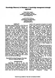
Knowledge Discovery in a Dairy Cattle Database (Mining for predictive models) H.A. Abbass1 P.E. Macrossan2 M. Towsey1 K. Mengersen2 G. Finn1 Queensland University of Technology, School of Computing Science, Machine Learning Research Centre, Data Mining Lab, GPO Box 2434, QLD 4001, Australia. 2 Queensland University of Technology, Department of Mathematical Sciences, GPO Box 2434, QLD 4001, Australia. 1
Technical Report: TR-FIT-99-01
Abstract. Proper design of a breeding program has been an issue of pri-
mary concern in much animal breeding research during the last decade. Data Mining (DM) is a powerful paradigm for nding patterns that can be used to predict the productivity of progeny given information about their sire, dam and the environment. The more accurate the discovered patterns, the more genetic gain one can achieve in a breeding program. This paper describes a DM process on an Australian dairy database. The focal point of this paper is the selection of a point estimation model for predicting the daughter milk yield within an intelligent decision support system, currently being developed for the Australian dairy industry. The selection of the minimum number of attributes, su�cient for satisfactory prediction, and of an accurate mining algorithm form the overall objective of the paper. In addition, the advantages of Bayesian neural networks over conventional feed-forward neural networks are explored.
1 Introduction The dairy industry in Australia is one of the country's main agricultural resources. In 1995-96, there were 13,888 dairy farms nationwide (Source: Australian Dairy Corporation) with 1.924 million dairy cows and a total milk production of 8.7 billion litres with a value of $AUD3 billion (Source: Australian Bureau of Statistics). Increases in productivity come from e�cient breeding programs and improved management practices. During the last decade, decision support systems have been developed to increase productivity in the dairy industry. Previous studies [10, 6] have shown the potential of using Neural Networks (NNs) as part of an animal breeding program to determine which cows should be selected for breeding in a given year and which should be culled. The Victorian Department of Agriculture [4] developed a computer program "Selectabull" for selecting the most suitable bulls for breeding into a farmer's herd and ranking them according to the predicted pro tability of the progeny of each. The program depends on
the Australian Breeding Values (ABVs) which measure an animal genetic potential. Given the low heritability of milk, fat, and protein, it is clear that the ABVs for these attributes are not su�cient for better decision-making. Moreover, ABVs are calculated using the Best Linear Unbiased Predictor (BLUP), which assumes that the relations between di�erent traits are linear. Another system, "ConnectiBull" [5], was developed by the Machine Learning Research Centre at the Queensland University of Technology. However, ConnectiBull is designed around an NN speci c for each bull and therefore su�ers from being bull speci c. Although BLUP predicts the expected genetic merit of an animal trait and we predict the expected phenotype of this trait, the phenotypic value is obtained by adding the average herd production value of this trait to its genotypic value. Since the herd average is constant within a herd, the output of our prediction model is comparable with the output of BLUP assuming that BLUP will use the same data set we have. The motivation for this paper is to investigate the assumptions of BLUP, that is the linearity assumption underlying the predictive model, with the aim of selecting a suitable predictive model for an Intelligent Decision Support System (IDSS) [3, 1, 2], currently being developed by the authors, in conjunction with the Queensland Department of Primary Industries, for the Australian dairy industry. The aim is to investigate whether the use of NNs can improve the accuracy of the prediction as a result of some nonlinearity in the data. The predictive model predicts the rst lactation milk volume for the progeny using information about its sire, dam, and the environment. Three objectives are identi ed, 1. identifying the minimum number of attributes appropriate for a satisfactory predictive accuracy, 2. testing the e�ect of data pre-processing on the predictive model, and 3. selecting the most suitable method for prediction which can be e�cient in an IDSS, that is, a method that works with the least amount of user interaction and gives accurate prediction. Data Mining (DM) is a powerful paradigm to achieve the objective of the paper. In this paper, the DM process is presented in two stages. Section 2 covers the rst stage, data and algorithm engineering, and the second stage, the mining experiments and results, is decomposed into three computational experiments in Sections 3, 4, and 5. Conclusions are then drawn in Section 6.
2 Data and Algorithm Engineering 2.1 Data Selection and Extraction
The database used for these experiments is extracted from an ADHIS (Australian Dairy Herd Improvement Scheme) database which covers the years 1993-95 and
contains 48 plain text les with over 80 million records occupying 6 Gigabytes of disk storage. The various les contain cow ABVs, workability traits, sire ABVs, production lactations and test days, cow pedigree, and herd data. Files for the Australian State of Victoria are selected for the following reasons: 1. Over 70% of the available data comes from Victoria, which accounts for more than 60% of the dairy industry in Australia. 2. It has limited environmental variation. 3. It is representative of managerial e�cacy as it covers a wide range of farm types from small to large commercial ones. After an extraction process, we had data, covering 700,000 cows (dams and daughters), for 5.5 million lactation test day records with total productions for each cow during her lactation period estimated from measurements taken on about 19 million test days records. As determined by a domain expert, insigni cant as well as redundant elds were excluded and 59 elds are selected out of the 154 elds in the les. The selected data were ltered to omit: 1. records that contained missing values in the selected elds. For example, records in the cow pedigree le lacking information about parent age, cows with no listed daughters, or daughters with no listed mothers. 2. records that did not pass the validation requirement that the recorded date of birth be at least two years earlier than the recorded date of rst lactation. 3. records of cows with few test days (less than 7) since estimating cow yields using few test days is unreliable. After ltering, there remained a subset of records we judged to be su�cient for mining. The records of lactation test days, when actual milking yields are measured, were used to estimate the standard 300-day milk production. The mean and standard deviation of the milk yield for each herd in the database were then calculated as implicit indication of the conditions of managerial practice and physical environment of the herd. A composite table of 25,678 records suitable for the mining objective was constructed by merging the individual tables to obtain complete records of information for each cow. Each row in the table includes daughter and dam identi cation information and production gures for the rst and up to two subsequent lactations of each animal. In addition the records contain sire and herd information. Redundancies in the merged table are necessary since, for example records for siblings contain duplicate parental information. Each record contains 16 elds of daughter information, 23 elds for her dam, and 20 for her sire making 59 elds in total for use in our experiments.
2.2 Feature Selection We di�erentiate between rst lactation milk volume, FLMV, and second lactation milk volume, SLMV, since there is a di�erence in the productivity of the animal over age. Twelve features tentatively judged to have an impact on the output variable FLMV, were identi ed with the aid of the domain expert. From these, we identi ed four sets of features that appeared to be most suitable for study. The rst feature set contains all twelve features as shown in the rst row of Table 1. The second excludes sire ABV reliability and ABV milking speed, since they are weakly correlated with the dependent variable (correlation coef cients are 0.10 and 0.08 respectively), herd mean FLMV, and protein and fat yields, because their high correlation with dam milk yield renders them largely redundant (0.70, 0.93, and 0.80 respectively). The third feature set is derived from the second by excluding the Australia Selection Index (ASI), since it has low correlations with daughter FLMV (0.10), and the ABV for survival, as it seemed to have no e�ect on daughter FLMV (correlation coe�cient is 0.02). The fourth feature set is in turn derived from the third by excluding all sire ABV production information leaving only the dam SLMV and the herd mean Not FLMV for prediction. The four features are summarised in Table 1.
Feature Set
Network Input Features
1
Herd mean Not FLMV, Herd mean FLMV, Dam SLMV, Dam second fat, Dam second protein, ABV milk, ABV fat, ABV protein, Reliability, ASI, ABV milking speed, ABV survival. 2 Herd mean not FLMV, Dam SLMV, ABV milk, ASI, ABV survival. 3 Herd mean not FLMV, Dam SLMV, ABV milk. 4 Herd mean not FLMV, Dam SLMV. Table 1. The four initial feature set
2.3 Experimental Design We attempt to discover a predictive model for daughter FLMV using the least possible number of input features. Since the predictive model is a component in an intelligent decision support system, the selected algorithm should more-or-less work independently under normal conditions. In addition, it should be accurate and able to mine the database with minimal user interaction. Accordingly, three types of point estimation methods linear regression (LR), NN, and Bayesian
neural network (BNN), have been selected for comparison. LR was included as it is a reliable statistical technique that does not need initial settings or prior distributions. NNs were included because of their adaptive behaviour and their ability to approximate nonlinear trends in the data. A Bayesian framework was applied to the NN to investigate claims by various authors of advantages over traditional NN learning [8].
Recalling the three objectives of the paper; experiment 1 in Section 3 covers the rst objective, identi cation of the minimum number of attributes appropriate for a satisfactory predictive accuracy. Experiment 2 in Section 4 covers the second objective, the e�ect of data preprocessing on the predictive model. The third experiment in Section 5 investigates the last objective, the selection of the most suitable method for prediction. The three mining experiments have been designed with 80% of the data used for constructing the model and the remaining 20% for testing the generalisation of the model.
3 Experiment 1: Feature Set Selection In this experiment, the objective is to select one of the four feature sets which accurately predict daughter FLMV. Correlation coe�cients between di�erent elds in Table 1 and daughter FLMV (the target of the prediction) were calculated to gain insight. The highest correlation (0.76) was found between the daughter FLMV and the average herd mean FLMV which means the mean herd milk production including that produced by cows lactating for the rst time (including the daughters). This variable is found to be irrelevant since, as we mentioned before, daughter FLMV was used in calculating it. A high correlation was also found between the daughter FLMV and its season of calving [7]. However, it was decided not to include any information about the daughter amongst the input features since in reality the daughter performance is predicted before the dam is mated. Each feature set is tested using a xed-architecture feed-forward NN with a single hidden layer of three units. All the inputs and the output were linearly normalised between 0-1. The average predicted performance for daughter FLMV of 10 trained NNs on the four feature sets, listed in Table 1, is presented in Figure 1 together with the distribution of the original data and the prediction using LR. The root mean square error (RMSE) and the correlation coe�cients, r(NN,target), between network predictions and target values are listed in columns 3 and 4 of Table 2. The rst feature set produces a slightly higher correlation coe�cient between NN prediction and the target at the cost of having nine additional variables. Further analysis revealed that the di�erence of (0.02) in the correlation coe�cient between the rst and second feature set was due to herd mean FLMV. We decided not to include this variable since daughter FLMV, the dependent variable in the model, is used in the calculations of this
average. Feature set 3 was chosen as the preferred feature set with two production features viz. dam SLMV and sire ABV milk, and one environmental feature, herd average milk volume excluding rst lactation (herd mean Not FLMV). This alone agreed with the domain expert's principle that parental achievements together with the physical and managerial environment are strongest determinants of daughter production traits. The outcome of this experiment is to use the dam SLMV, sire ABV, and herd not FLMV as the feature set for prediction.
b. 3 inputs 800
600
600
frequency
frequency
a. 2 inputs 800
400
200
0
400
200
0
2000
4000 6000 milk
8000
0
10000
0
2000
800
600
600
400
200
0
8000
10000
8000
10000
d. 12 inputs
800
frequency
frequency
c. 5 inputs
4000 6000 milk
400
200
0
2000
4000 6000 milk
8000
10000
0
0
2000
4000 6000 milk
Fig. 1. The performance of di�erent feature sets using NN. The target is represented by (|) whereas the LR prediction by (�), and the NN prediction by ( ). :::
Feature Number of RMSE of NN r(NN,target) Set Attributes
1 12 754 0.78 2 5 766 0.76 3 3 761 0.76 4 2 773 0.75 Table 2. The RMSE and correlation coe�cient between the target (daughter FLMV) and the output of the NN on the test set for each feature set
4 Experiment 2: E�ect Of Data Pre-Processing It is common practice in the dairy industry [9] to correct milk production values for age, since mean production yields vary with age at lactation. We investigate the e�ects of age and season correction on the accuracy of the prediction. The production traits are corrected for the e�ect of age and the season of calving is included as an input since it was di�cult to identify its trend from the available data. Consequently, the features dam second lactation milk volume (SLMV) and the daughter rst lactation milk volume (FLMV) which we used needed to be corrected for age. The correction factor, CF, is calculated as CF = MV (mature)=MV (group), where MV (mature) is the average milk volume (MV) of all mature cows aged 5 to 7 years (when production is at a peak) and MV (group) is the average MV of all cows in the age group being corrected. Cows were grouped by age where each age group is of one year length. In Figure 2, we show the average dam SLMV as a function of age before and after age correction. It can be seen by comparing Figures 2a and 2b that the correction removes a small nonlinear trend, representing the e�ect of cow age on its milk production.
(B) 9000
8000
8000
7000
7000
SLMV
SLMV
(A) 9000
6000
6000
5000
5000
4000
4000
3000
40
60
80
100 AGE
120
140
160
3000
40
60
80
100 AGE
120
140
160
Fig. 2. The impact of age correction on dam SLMV. At left (a) Dam SLMV before age corrections as a function of age in months. At right (b) Dam SLMV after age corrections as a function of age in months.
In Table 3, the e�ect of age correction and the inclusion of season of calving to the inputs is presented. The performance of the NN changed slightly, thus may indicate that the trends caused by age and season in the dam SLMV and the output daughter FLMV are super uous for the NN. On the contrary, linear regression was sensitive to these changes and its performance improved. This is an important nding since the correction for factors, such as age or season, as preprocessing for BLUP is very essential for its performance though with NN, this
might not be the case. In the rest of this paper, the corrected feature set (dam SLMV corrected for age, sire ABV, herd not FLMV, and season of calving) is used as the input set and daughter FLMV corrected for age is used as the target.
Inputs LR-RMSE ( ) NN-RMSE ( ) Without Age correction 787 0.72 761 0.76 or the season With age correction and season 762 0.76 761 0.77 Table 3. Comparing the e�ect of age correction and the addition of season of calving to the third feature set using three hidden units. r LR; target
r N N; target
Another component of pre-processing is normalisation of features. When using NN, it is important to ensure that each numeric value (especially for the output when the range of values for the output is larger than the range of values for the activation function) is normalised. We considered three normalisation transformations for continuous variables. These are linear normalisation between [0,1], the Z-transform, and a transformation we dub uniform-Z. In uniform-Z, the inputs are normalised in the range [0,1] using the cumulative normal distribution function whereby production traits are transformed to the value of the accumulated probability of occurrence for a normal distribution of mean and variance equal to those of the population for the production trait. The e�ect of the uniform-Z transformation is shown in Figure 3 where we can see that uniform-Z spreads the data over the normalised range [0,1] more or less uniformally. NNs are trained for each normalisation method on ve di�erent architectures having 1,2,3,4, or 7 hidden units. NNs for the rst and third normalisation employ a sigmoid output unit so that the output is likewise normalised in [0,1]. For the second normalisation, where the variables do not always lie between 0 and 1, a simple linear unit is more suitable. We employ seven input units: herd milk mean average, Dam SLMV corrected for age, Sire ABV milk, and four sparsely coded inputs for the seasons, spring, summer, winter, and autumn. In each case, 10 NNs with di�erent weight initialisations are trained for 20,000 epochs and tested on the test set every 50 epochs for a learning rate of 0.03 and zero momentum. The correlation coe�cient between the output of each network and the target is calculated and used along with the RMS error as an indication of the predictive accuracy as shown in Table 4. In all network architectures, the linear normalisation is found to produce the best performance followed by Z-transform and the uniform Z transform. For linear normalisation, the correlation coe�cient increases to a maximum of 0.77 and the RMS error decreases to a minimum for three hidden units.
(B) 4500
4000
4000
3500
3500
3000
3000
FREQUENCIES
FREQUENCIES
(A) 4500
2500
2000
2500
2000
1500
1500
1000
1000
500
500
0
0
2000
4000 6000 MILK INTERVAL
8000
10000
0
0
0.2
0.4 0.6 MILK INTERVAL
0.8
1
Fig. 3. The e�ect of uniform Z normalisation on the distribution of the data. At left (a) the histogram of the original data set with the milk volume intervals on the horizontal axis. At right (b) the histogram of the data normalised using uniform Z with the transformed milk volume on the horizontal axis. Normalisation Method
RMSE
r(NN,target)
Linear Normalisation 761 0.77 Z-transform Normalisation 785 0.76 Uniform Z Normalisation 789 0.76 Table 4. The correlation coe�cient between the output for the NN using 3 hidden units and the target and the RMSE values of di�erent normalisation methods using the third feature set with season as an input and age correction.
5 Experiment 3: Selection of Learning Algorithm BNN software obtained from [8] implements the Bayesian model using Markov Chain Monte Carlo methods (MCMC) to sample from the posterior distribution. We employ multi-layer perceptrons with seven input units representing herd not FLMV, dam milk yield, sire ABV milk, and four sparsely coded inputs representing the four seasons, one hidden layer of either 1,2, 3, 4, or 8 units with the tanh activation function, and a single output unit representing daughter FLMV adjusted for age. The data is normalised in the range [-1,1] since the BNN simulation software used employs the tanh activation function. The prior distributions [8] used for the network parameters were taken to be normally distributed N (0; !), with standard deviations ! considered to be hyperparameters with inverse Gamma, IG(�; ), distributions. Three network hyperparameters with distributions IG(0:05; 0:5) were speci ed, one for the input-tohidden weights, one for the hidden unit biases, and one for the hidden-to-output weights. The output unit bias was given a simple Gaussian prior N (0; 100). The value of the output unit was taken as the mean of a Gaussian distribution for
the target, with an associated error term (or network "noise") having a Gaussian prior N (0; �). The standard deviation of this error term was controlled using a hyperparameter with distribution IG(0:05; 0:5). The model was implemented using Markov Chain Monte Carlo methods to sample from the posterior distribution. In the initial state of the simulation, each of the hyperparameters (the input-to-hidden weights, the hidden unit biases, the hidden-to-output weights and the "noise" hyperparameters) was given a value of 0.5. The network parameters were given initial values of zero. Predictions were based on the nal 80 of 100 iterations, the rst 20 being discarded as "burn-in". The software used to implement the BNN, and the particulars of the implementation used, are described by Neal [8]. In Table 5, we present results for LR and NN for feature set 3, after adding the season e�ect, as well as for BNN. As can be seen from Table 5, the behaviour of LR, BNN, and NN is very similar. However, we plotted the distribution of the output in each case and we noticed that neither NN nor BNN is able to produce exactly the distribution generated by LR. Moreover, BNN succeeded in generating the same mode as LR, and NN had a smaller standard deviation than BNN or LR. The curve for LR lies mostly between NN and BNN.
Criteria
LR
NN
BNN
Correlation 0.76 0.77 0.77 RMS error 762 761 761 Table 5. The correlation coe�cient between the output of LR, NN, and BNN and the target along with the RMSE values for each method. The NN results are the average over ten di�erent runs with di�erent weight initialisations. Both NN and BNN results are with three hidden units.
6 Discussion On the one hand, when the data is linear, NN and BNN produce the same level of predictive performance as LR. On the other hand LR cannot handle nonlinearity in the data set. In an IDSS which should contain a predictive model that is capable of working independently under a range of circumstances, a choice of BNN or NN is more appropriate. Moreover, although it may take longer to train a BNN than a single conventional NN, typically conventional NN training requires multiple training runs with di�erent initial weights and trying di�erent learning parameters. Accordingly, BNNs seem to be faster than conventional NNs which is an important advantage for the nal IDSS. In summary, we believe that the BNNs are more suitable in our case.
In this paper, the process of mining for predictive patterns in a dairy database is described. It is found that neural networks are capable of ignoring the trend of some factors, such as the age and season, whereas the performance of LR was sensitive to these corrections. In addition, Bayesian neural networks are found to be capable of approximating the posterior distributions of neural network parameters, bias and weights, even with arbitrary prior distributions. Moreover, they are found to be insensitive to the network topology as NN. Finally, the linear assumption underlying BLUP is found valid only if the data is corrected; otherwise, a neural network will be more suitable.
7 Acknowledgement We wish to thank Dr. Mick Tierney from the department of primary industries, Queensland, for his valuable comments. This work was done as a part of an ARC collaborative grant number C19700273.
References 1. H.A. Abbass, W. Bligh, M. Towsey, M. Tierney, and G.D. Finn. Knowledge discovery in a dairy cattle database: automated knowledge acquisition. Fifth International Conference of the International Society for Decision Support Systems (ISDSS'99), Melbourne, Australia, 1999. 2. H.A. Abbass, M. Towsey, and G.D. Finn. An intelligent decision support system for dairy cattle mate-allocation. Proceedings of the third Australian workshop on Intelligent Decision Support and Knowledge Management, pages 45{58, 1998. 3. H.A. Abbass, M. Towsey, and G.D. Finn. OR and data mining for intelligent decision support in the Australian dairy industry's breeding program. Proceedings of New Research in OR, ASOR, Brisbane, pages 1{23, 1998. 4. P.J. Bowman, P.M. Visschert, and M.E. Goddard. Customized selection indices for dairy bulls in australia. Animal Science, 62:393{403, 1996. 5. G.D. Finn, R. Lister, R. Szabo, D. Simonetta, H. Mulder, and R. Young. Neural networks applied to a large biological database to analyse dairy breeding patterns. Neural Computing and Applications, 4:237{253, 1996. 6. R. Lacroix, F. Salehi, X.Z. Yang, and K.M. Wade. E�ects of data preprocessing on the performance of arti cial neural networks for dairy yield prediction and cow culling classi cation. Transactions of the ASAE, 40:839{846, 1997. 7. P.E. Macrossan, H.A. Abbass, K. Mengersen, M. Towsey, , and G. Finn. Bayesian neural network learning for prediction in the Australian dairy industry. Lecture Notes in Computer Science LNCS1642, Intelligent Data Analysis, 1999. 8. R.M. Neal. Bayesian Learning for Neural Networks, Lecture Notes in Statistics No 11. Springer-Verlag, 1996. 9. G.H. Schmidt and L.D. Van Vleck. Principles of Dairy Science. W.H. Freeman and Company, 1974. 10. K.M. Wade and R. Lacroix. The role of arti cial neural networks in animal breeding. The Fifth World Congress on Genetics Applied to Livestock Production, pages 31{34, 1994.