Knowledge in Communication Networks

Knowledge in Communication Networks Jia Tao∗

Pavel G. Naumov⋆

November 3, 2015

Abstract The article investigates epistemic properties of information flow under communication protocols with a given topological structure of the communication network. The main result is a sound and complete logical system that describes all such properties. The system consists of a variation of the multi-agent epistemic logic S5 extended by a new network-specific Gateway axiom.

1

Introduction

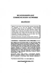
In this article we study epistemic properties of communication protocols. Consider, for example, a protocol P1 between agents p, q, u, and v. Under this protocol, agent p communicates to agent q a message over a secure communication channel m. Next, agent q must communicate the same message over insecure channels to agent u. To achieve this, agent q chooses a random onetime encryption pad (“key”) and computes a ciphertext as a bit-wise sum of the message and the key modulo 2. Agent q then sends the key and the ciphertext to agent u over insecure channels k and c accordingly. Finally, agent u, upon receiving the key and the ciphertext, computes a bit-wise sum of these two strings modulo 2 and communicates the result over a secure channel m′ to agent v. 11001

p

01001 m

k q

10000 c

u

01001 m'

v

Figure 1: Run r1 of protocol P1 . ⋆ Department of Computer Science, Illinois Wesleyan University, Bloomington, Illinois, the United States, [email protected] ∗ Department of Computer Science, The College of New Jersey, Ewing, New Jersey, the United States, [email protected]

1

A run of a protocol is an assignment of values to all communication channels that satisfy the restrictions imposed by the protocol. An example of a run r1 of protocol P1 is depicted in Figure 1. Note that for any run satisfying the restrictions of P1 , the value of channel m is the same as the value of channel m′ . Thus, any outside observer who can eavesdrop on channel m under run r1 would be able to learn that channel m′ has a value of 01001 on this run. Using epistemic modal logic notations1 , we write this as r1 ⊩ 2m (m′ = 01001). At the same time, since there is no connection between the values of the ciphertext c and the original message m, an external observer eavesdropping on channel c would not be able to deduce the value of channel m′ :

Similarly,

r1 ⊩ ¬2c (m′ = 01001).

(1)

r1 ⊩ ¬2k (m′ = 01001).

(2)

We now consider a variation of protocol P1 that we call P2 . Under the second protocol agents q and u are allowed to make a mistake in at most one bit during the encryption and the decryption stages respectively. In other words, the Hamming distance between the value of channel c and the bit-wise sum of values of channels m and k is no more than one. Similarly, the Hamming distance between the value of channel m′ and the bit-wise sum of values of channels c and k is no more than one. An example of a run r2 of protocol P2 is depicted on Figure 2. 11001

p

01001 m

k q

10100 c

u

11101 m'

v

Figure 2: Run r2 of protocol P2 . Note that run r1 is also a valid run of protocol P2 . Thus, an external observer eavesdropping on channel m on run r2 is not able to distinguish run r2 from run r1 . Hence, such an observer would not be able to conclude that the value of m′ is 11101. Therefore, under protocol P2 , r2 ⊩ ¬2m (m′ = 11101). At the same time, an external observer eavesdropping on channel m on run r2 of protocol P2 should be able to conclude that the value of channel m′ is not 1 Similarly to Kane and Naumov [1], we interpret modality 2 m as “any outside observer who can eavesdrop on channel m knows that . . . ”, instead of more traditional “agent m knows that . . . ” [2].

2

01110 because the Hamming distance between 01001 and 01110 is three and, according to the restrictions of protocol P2 , errors could be introduced in at most two bits during the encryption and the decryption stages combined: r2 ⊩ 2m (m′ ̸= 01110). We now consider another variation of protocol P1 that we call P3 , see Figure 3. The original message m in this protocol is first encrypted into a cyphertext c using a key k, then it is recovered as m′ , then again encrypted and recovered as m′′ . A single bit-error could be introduced by each encryption and decryption stage. Thus, the Hamming distance between strings m and m′′ could be at most four. Figure 3 shows a possible run r3 of this protocol. 11001

p

m

11011

k

01001 q

10100 c

u

11101 m'

k' v

00111 c'

s

11000 m''

t

Figure 3: Run r3 of protocol P3 . An external observer eavesdropping on channel m on run r3 under P3 would not be able to know the exact value of m′ . However, it would know that the value of channel m′ is at a Hamming distance no more than two from the value of m. Note that the Hamming distance between the value of m and the string 10110 is five. Thus, due to the triangle inequality, the observer would be able to conclude that the Hamming distance between the value of m′ and the string 10110 is at least three. Based on this, the observer would be able to conclude that any other observer eavesdropping on channel m′ should know that the value of m′′ is not equal to 10110: r3 ⊩ 2m 2m′ (m′′ ̸= 10110). So far we have discussed epistemic properties of individual runs. A property which is true on one run does not have to be true on another. For example, the above formula 2m 2m′ (m′′ ̸= 10110) is not true on any run in which the value of channel m is 10110. However, a similar property is true on all runs of protocol P3 : (m = 01001) → 2m 2m′ (m′′ ̸= 10110). (3) Another property true for all runs of protocol P3 is 2m′ (m ̸= 00000) → 2m′ (m′′ ̸= 00000).

(4)

Indeed, the assumption 2m′ (m ̸= 00000) tells us that an observer of channel m′ on the current run can conclude that m ̸= 00000. Since at most two mistakes can be introduced between channels m and m′ , we can conclude that the 3

message that the observer sees on channel m′ contains at least three digits of 1. Therefore, for a similar reason, this observer will conclude that m′′ ̸= 00000. A property true for all runs of one protocol does not have to be true for all runs of some other protocols. For example, property (3) is false under protocol where up to two bits could be corrupted during each encryption and each decryption stage. Property (4) is not true under a protocol where agents q and u, unlike agents s and t, are not allowed to make mistakes. In this article we study epistemic properties common to all protocols that have the same topological structure2 of communication networks. Consider, for example, property 2m (m′′ ̸= 00000) → 2m′ (m′′ ̸= 00000).

(5)

We will see later in this article that this property is true for each protocol where, as in Figure 3, communication between channels m and m′′ happens only through channel m′ . The above formula (5) involves inequality. Neither inequality nor equality is a part of the language of our system. We only allow propositional symbols as atomic statements. An example of an epistemic property common to all protocols with the network topology depicted in Figure 3 expressible in our language is: 2m 2m′′ φ → 2m′ 2m′′ φ. (6) Informally, this property states that if any observer eavesdropping on channel m is able to deduce that any other observer eavesdropping on channel m′′ can conclude that some property φ is true, then the same deduction can be made by any observer eavesdropping on channel m′ on the same run. This property, as shown in Example 3, is a special case of our Gateway axiom. We prove the soundness of Gateway axiom with respect to a formally defined semantics in Section 6. Another, perhaps surprising, example of a property common to all protocols with the network topology depicted in Figure 3 is: 2m′ (2m φ ∨ 2m′′ ψ) → 2m′ 2m φ ∨ 2m′ 2m′′ ψ.

(7)

Generally speaking, the knowledge of a disjunction of two formulas does not imply the knowledge of either of the two disjuncts. The above formula, however, states that this is true when the disjunct talks about the knowledge of observers located on different sides of channel m′ . In Section 5, we prove a more general form of property (7). An epistemic logic for reasoning about communication graphs was proposed by Pacuit and Parikh [3]. Their language consists of two different modalities: an epistemic modality Ka labeled by an agent a and a modality 2 interpreted as “after any sequence of communications under the given protocol it is true that”. They discussed logical principles specific to a given network topology 2 As we formally define in the next section, the topological structure of a communication network is an undirected graph with multiple edges.

4

and even gave, in the introduction, a principle similar to our Gateway axiom. However, they did not provide a complete axiomatization of their logical system for a specific topology, even though they proved its decidability. Kane and Naumov [1] proposed a similar logical system whose language contains only epistemic modality. They eliminated modality “after any sequence of communications” by assuming that all statements refer to the final knowledge after the communication. In this simplified setting they have been able to prove completeness theorem, but only for the case of linear communication networks. This article extends Kane and Naumov’s work from linear communication chains to arbitrary connected graphs. The logical system introduced in [1] contained two principles capturing topology of linear communication chains: Gateway axiom and Disjunction axiom, similar to properties (6) and (7) above. The more general version of Gateway axiom described in the current article no longer requires Disjunction property as a separate axiom. Instead, we prove this property from the more general version of Gateway axiom in Lemma 2. More importantly, the proof of the completeness theorem for non-linear graphs is completely different from the proof of completeness for linear communication chains. In the case of the proof of completeness for linear communication chains, if an observer of channel m knows certain information about channel m′ , then it is enough to simply pass this information along the interval between channels m and m′ . However, the same technique does not apply to non-linear graphs. As we have demonstrated with protocol P1 and properties (1) and (2), in nonlinear graphs an observer of channel m might know certain information about channel m′ without anyone between them knowing this information. To be able to prove completeness for non-linear graphs we introduce a new network flow construction described in Section 7. An applied value of the result in this article is in providing a uniform protocol design procedure for communication networks. Namely, suppose that one needs to design a protocol for a network that satisfies security conditions φ1 ,. . . , φn expressed in our modal language. Assume additionally that the physical layout (topological structure) of the network is given and can not be changed. In such ∧ a setting, the protocol designer should be able to either (i) derive formula i≤n φi → ⊥ in our logical system and, thus, prove that the specification of the protocol can not be met, or (ii) use the construction from our proof of completeness to produce a protocol that satisfies each of the desired conditions φ1 ,. . . , φn . Tao, Slutzki, and Honavar [4] introduced a conceptual logical framework for answering queries without revealing secrecy to multiple querying agents where there is a set of secrets that need to be protected against each of these agents. The communication between agents is modeled using a graph. The focus of their work is on a privacy-preserving algorithm, not on an axiomatic system. This article is also related to the works on information flow on graphs [5, 6, 7, 8, 9, 10], that study properties of nondeducibility, functional dependency, common knowledge, and fault tolerance predicates. Unlike those works, this article is using a modal language. The article is organized as follows. Section 2 introduces relevant terminology 5

from graph theory. Section 3 defines the formal syntax and the semantics for our logical system, which is introduced in Section 4. Section 5 illustrates our logical system by giving several examples of formal proofs in this system. Some of these examples are used later in the proof of completeness. The soundness of the system is established in Section 6. The rest of the article is dedicated to the proof of completeness in Section 7. The proof starts with an informal discussion of a network flow protocol. It continues to formalize the network flow protocol as a canonical communication protocol over the graph. Finally, multiple instances of the canonical protocol are aggregated together to show the completeness of the logical system. Section 8 concludes the article.

2

Graph Theory Preliminaries

We study epistemic properties common to all protocols with the same topology of a channel network. Under such a protocol, multiple messages can be sent over the same channel. A value of a channel is the set of all messages communicated through the channel, possibly in both directions. We specify the network topology as an undirected graph in which vertices represent agents and edges represent communication channels between agents. In this section we introduce graph terminology used throughout the rest of the article. Graph (V, E) contains a set of vertices V and a set of edges E with an incidence relation between them. We allow loops and multiple edges between the same pair of vertices. We write e ∈ Edge(v0 , v1 ) to state that edge e ∈ E is one of (possibly multiple) edges between vertices v0 ∈ V and v1 ∈ V . By Inc(v) we denote the set of all edges incident to vertex v ∈ V . By Inc(e) we denote the set consisting of the two ends of edge e ∈ E. For example, Inc(q) = {m, k, c} and Inc(k) = {q, u} in Figure 3. Let e ∈ E be an edge of a graph (V, E) incident to a vertex v ∈ V . If edge e is removed from the graph, remaining graph (V, E \ {e}) might have up to two connected components. By C-ve we denote the connected component of the graph (V, E \ {e}) that contains vertex v. Note that in some cases component C-ve might be equal to the entire graph (V, E \ {e}). For the graph in Figure 3, component C-um′ consists of vertices p, q, and u as well as edges m, k, and c. For the same graph, component C-uk contains all vertices of the original graph and all edges of that graph except for edge k. A path is a sequence e0 , v1 , e1 , . . . , vk , ek such that k ≥ 0, e0 , . . . , ek are distinct edges, and v1 , . . . , vk are distinct vertices of the graph such that ei , ei+1 ∈ Inc(vi+1 ) for each 0 ≤ i < k. In Figure 3, sequence k, u, m′ , v, c′ and oneelement sequence c are both examples of paths. A circular path is defined similarly except for edges e0 and ek being the same. Definition 1 Edge g is a gateway between sets of edges A and B of a graph if each path that starts with an edge in set A and ends with an edge in set B contains the edge g.

6

For example, edge m′ is a gateway between sets of edges {m, k} and {k ′ , c′ } in Figure 3. Note that in the above definition edge g can belong to either or both of the sets A and B. In Figure 3, edge k is a gateway between singleton set {k} and set {m, m′′ }.

3

Syntax and Semantics

In this section we define the language and the formal semantics of our logical system. These definitions presuppose a fixed signature of the communication network. Definition 2 A signature Sig is an arbitrary triple Sig = (V, E, {Pe }e∈E ), such that (V, E) is a connected graph and {Pe }e∈E is a family of disjoint sets of propositions. Informally, propositions in set Pe are atomic statements about values of the communication channel e. Different connected components of a disconnected graph can not exchange any information between them, so, for the sake of simplicity, we have chosen to restrict our system to connected graphs. We next define the language of our logical system. Definition 3 For every signature Sig, let Φ(Sig) be the minimal set of formulas such that 1. ⊥ ∈ Φ(Sig), 2. Pe ⊆ Φ(Sig) for every e ∈ E, 3. if φ, ψ ∈ Φ(Sig), then φ → ψ ∈ Φ(Sig), 4. if e ∈ E and φ ∈ Φ(Sig), then 2e φ ∈ Φ(Sig). We assume that connectives ¬, ∧, and ∨ are defined through → and ⊥ in the usual way. Informally, a protocol is specified by giving a range of values3 for each edge (“communication channel”) and establishing dependencies between the values of the edges. These dependencies are “enforced” by vertices (“agents”), and, thus, each such condition only involves edges incident to a vertex. For this reason we refer to these conditions as “local”. For example, for protocol P1 in the introduction, the local condition enforced by vertex q is c = m ⊕ k, where m⊕k is a bit-wise exclusive or of binary strings transmitted over channels m and k. For protocols P2 and P3 , the local condition at vertex q is h(c, m ⊕ k) ≤ 1, where h(·, ·) denotes the Hamming distance between any two binary strings of the same length. The local condition for vertex p under all three of the above 3 Each

value represents the collection of all messages sent through the channel on a given

run.

7

protocols is the constant true. In the formal definition below, a local condition is treated not as a Boolean function but rather as a set of tuples on which this function is true. Recall that each atomic proposition p in set Pe is viewed as proposition “about” the value of channel e. In what follows, by π(p) we informally mean the set of all values of channel e for which proposition p is true. Definition 4 A protocol over a signature (V, E, {Pe }e∈E ) is a tuple ({We }e∈E , {Lv }v∈V , π) such that 1. for every edge e ∈ E, set We is an arbitrary set of values, ∏ 2. for every v ∈ V , set Lv ⊆ e∈Inc(v) We specifies local conditions at vertex v, 3. for every p ∈ Pe , function π is such that π(p) ⊆ We . We denote π(p) by pπ . Definition∏5 A run of a protocol ({We }e∈E , {Lv }v∈V , π) is an arbitrary tuple ⟨we ⟩e∈E ∈ e∈E We such that ⟨we ⟩e∈Inc(v) ∈ Lv for every v ∈ V . Definition 6 For any two tuples r = ⟨we ⟩e∈E and r′ = ⟨we′ ⟩e∈E and any f ∈ E, we write r =f r′ if wf = wf′ . Corollary 1 Relation r =e r′ is an equivalence relation.

⊠

The formal semantics of our logical system is defined in terms of runs of a protocol, rather than in more common terms of epistemic worlds of a Kripke model. Note, however, that any protocol can be viewed as a Kripke model in which runs of the protocol are epistemic worlds and equality of runs on a given channel c is the indistinguishability relation ∼c on epistemic worlds. Definition 7 For every signature Sig = (V, E, {Pe }e∈E ), every φ ∈ Φ(Sig), every protocol P = ({We }e∈E , {Lv }v∈V , π) over graph (V, E), and every run r = ⟨we ⟩e∈E of P, relation r ⊩ φ is defined recursively as: 1. r ⊮ ⊥, 2. r ⊩ p if we ∈ pπ , where p ∈ Pe , 3. r ⊩ ψ → χ if r ⊮ ψ or r ⊩ χ, 4. r ⊩ 2e ψ if r′ ⊩ ψ for every run r′ of P such that r′ =e r. For any signature Sig and any set of edges T , by Φ(Sig, T ) we mean the set of all formulas in Φ(Sig) in which all outermost modalities are labeled only by edges ∪ in T and all atomic propositions outside of scopes of all modalities belong to t∈T Pt . For example, 2a 2b φ → 2c ψ ∈ Φ(Sig, {a, c}). Also, if p ∈ Pa and q ∈ Pb , then 2b p → q ∈ Φ(Sig, {b}). We use this notation to state our Gateway axiom in the next section. Below is the formal definition of this notation. 8

Definition 8 For every signature Sig = (V, E, {Pe }e∈E ) and every T ⊆ E, let Φ(Sig, T ) be the minimal set of formulas such that 1. ⊥ ∈ Φ(Sig, T ), 2. Pt ⊆ Φ(Sig, T ) for every t ∈ T , 3. if φ, ψ ∈ Φ(Sig, T ), then φ → ψ ∈ Φ(Sig, T ), 4. if t ∈ T and φ ∈ Φ(Sig), then 2t φ ∈ Φ(Sig, T ). Note that in item 4 above, formula φ is an element of set Φ(Sig) rather than set Φ(Sig, T ).

4

Logical System

In this section we specify the axioms and the inference rules of our logical system for a given signature Sig = (V, E, {Pe }e∈E ). Our logical system, in addition to propositional tautologies in language Φ(Sig), contains the following axioms: 1. Truth: 2e φ → φ, where φ ∈ Φ(Sig), 2. Positive Introspection: 2e φ → 2e 2e φ, where φ ∈ Φ(Sig), 3. Negative Introspection: ¬2e φ → 2e ¬2e φ, where φ ∈ Φ(Sig), 4. Distributivity: 2e (φ → ψ) → (2e φ → 2e ψ), where φ, ψ ∈ Φ(Sig), 5. Gateway: 2e (φ → ψ) → (φ → 2g ψ), where e ∈ A, φ ∈ Φ(Sig, A), ψ ∈ Φ(Sig, B), and edge g is a gateway between sets of edges A ⊆ E and B ⊆ E. Note that axioms of Truth, Positive Introspection, Negative Introspection, and Distributivity are identical to the corresponding axioms of multi-agent epistemic logic S5. Thus, our logical system can be viewed as an extension of S5 by Gateway axiom.

g

e

B

A

Figure 4: Edge g is a gateway between sets of edges A and B.

Figure 4 illustrates the setting for Gateway axiom. To explain the intuition behind Gateway axiom, let us first consider the special case of this axiom when 9

formula φ is a propositional tautology. In this case, Gateway axiom can be reduced to 2e ψ → 2g ψ, which means that if an agent eavesdropping on channel e knows something about the channels in set B, then an agent eavesdropping on gateway channel g must also know this. Intuitively, this claim is true because the information about channels in set B can only reach the observer of channel e by flowing through the gateway channel g. However, to the best of our knowledge, Gateway axiom in this reduced form 2e ψ → 2g ψ does not yield a complete logical system. To achieve the completeness, we need a slightly more general principle that takes into account the “local” information about channels on the same side of the gateway as channel e. In Gateway axiom 2e (φ → ψ) → (φ → 2g ψ) the local information is captured by formula φ. We write ⊢Sig φ if formula φ is provable in our logical system for signature Sig using Modus Ponens and Necessitation inference rules: φ→ψ

φ,

φ 2e φ

ψ

where φ, ψ ∈ Φ(Sig) and e ∈ E. We write X ⊢Sig φ if formula φ is provable in our logical system from the set of assumptions X using only Modus Ponens rule. We omit subscript Sig when its value is clear from the context.

5

Examples

The soundness and the completeness of our logical system will be established in the next two sections. In this section we give several examples of formal proofs in this system. Among these examples there are several lemmas that will be used later in the proof of completeness. a

b

c

Figure 5: Three-Channel Linear Communication Network.

Example 1 For any signature Sig = (V, E, {Pe }e∈E ) and any φ ∈ Φ(Sig) where (V, E) is the graph depicted in Figure 5, ⊢Sig 2a (2b φ ∨ 2c φ) → 2b φ. In other words, if an observer eavesdropping on channel a knows that an observer eavesdropping on channel b knows φ or an observer eavesdropping on channel c knows φ, then the observer eavesdropping on channel b must know φ. Proof. Formula 2c φ → φ is an instance of Truth axiom. Thus, by Necessitation inference rule, ⊢ 2b (2c φ → φ). Hence, by Distributivity axiom and Modus Ponens inference rule, ⊢ 2b 2c φ → 2b φ. (8) 10

At the same time note that edge b is a gateway between sets {a, b} and {c}. Additionally, ¬2b φ ∈ Φ(Sig, {a, b}) and 2c φ ∈ Φ(Sig, {c}). Thus, by Gateway axiom, ⊢ 2a (¬2b φ → 2c φ) → (¬2b φ → 2b 2c φ). Hence, using statement (8) and the laws of propositional logic, ⊢ 2a (¬2b φ → 2c φ) → (¬2b φ → 2b φ). Note that formula (¬2b φ → 2b φ) → 2b φ is a propositional tautology. Thus, ⊢ 2a (¬2b φ → 2c φ) → 2b φ. Finally, recall that disjunction 2b φ ∨ 2b φ is an abbreviation for ¬2b φ → 2b φ. Therefore, ⊢ 2a (2b φ ∨ 2c φ) → 2b φ. ⊠

a

c

b

d

e

Figure 6: Five-Channel Linear Communication Network. In what follows, we denote by ⊤ the propositional tautology ⊥ → ⊥. Example 2 For any signature Sig = (V, E, {Pe }e∈E ) and any φ ∈ Φ(Sig) where (V, E) is the graph depicted in Figure 6, ⊢Sig 2a 2e 2c φ → 2b 2d φ. Proof. By Truth axiom, ⊢ 2c φ → φ. Thus, ⊢ 2d (2c φ → φ) by Necessitation inference rule. Hence, by Distributivity axiom and Modus Ponens rule, ⊢ 2d 2c φ → 2d φ.

(9)

At the same time, formula 2c φ → (⊤ → 2c φ) is a propositional tautology. Thus, by Necessitation rule, ⊢ 2e (2c φ → (⊤ → 2c φ)). By Distributivity axiom and Modus Ponens inference rule, ⊢ 2e 2c φ → 2e (⊤ → 2c φ).

(10)

Similarly, one can show that ⊢ 2a 2d φ → 2a (⊤ → 2d φ).

(11)

Since edge d is a gateway between the sets of edges {e} and {c}, ⊤ ∈ Φ(Sig, {e}), and 2c φ ∈ Φ(Sig, {c}), by Gateway axiom, ⊢ 2e (⊤ → 2c φ) → (⊤ → 2d 2c φ). Hence, using statement (9), statement (10) and the propositional reasoning, ⊢ 2e 2c φ → 2d φ. Thus, by Necessitation inference rule, ⊢ 2a (2e 2c φ → 2d φ). Then, by Distributivity axiom and Modus Ponens inference rule, ⊢ 2a 2e 2c φ → 2a 2d φ.

(12)

Since edge b is a gateway between sets of edges {a} and {d}, ⊤ ∈ Φ(Sig, {a}), and 2d φ ∈ Φ(Sig, {d}), by Gateway axiom, ⊢ 2a (⊤ → 2d φ) → (⊤ → 2b 2d φ). Therefore, using statement (11), statement (12), and the propositional reasoning, ⊢ 2a 2e 2c φ → 2b 2d φ. ⊠ We next prove formula (6) stated in Section 1. 11

Example 3 For any signature Sig = (V, E, {Pe }e∈E ) and any φ ∈ Φ(Sig), where G = (V, E) is the graph depicted in Figure 3, ⊢Sig 2m 2m′′ φ → 2m′ 2m′′ φ. Proof. Formula 2m′′ φ → (⊤ → 2m′′ φ) is a propositional tautology in language Φ(Sig). Thus, by Necessitation inference rule, we have ⊢ 2m (2m′′ φ → (⊤ → 2m′′ φ)). By Distributivity axiom and Modus Ponens inference rule, ⊢ 2m (2m′′ φ) → 2m (⊤ → 2m′′ φ)).

(13)

Note now that edge m′ is a gateway between sets of edges {m} and {m′′ }. Also, ⊤ ∈ Φ(Sig, {m}) and 2m′′ φ ∈ Φ(Sig, {m′′ }). Thus, by Gateway axiom, ⊢G 2m (⊤ → 2m′′ φ) → (⊤ → 2m′ 2m′′ φ). Hence, using statement (13), by the laws of propositional logic, ⊢G 2m 2m′′ φ → (⊤ → 2m′ 2m′′ φ). Therefore, again using propositional logic, ⊢G 2m 2m′′ φ → 2m′ 2m′′ φ. ⊠ Instead of proving property (7) from the introduction, in Lemma 2 we prove a slightly more general statement that later will be used in the proof of completeness. The proof of Lemma 2 relies on the following auxiliary lemma. Figure 4 illustrates the settings of both of these lemmas. Lemma 1 ⊢ 2e (φ ∨ ψ) → (φ ∨ 2g ψ), where edge g is a gateway between sets of edges A and B, e ∈ A, φ ∈ Φ(Sig, A), and ψ ∈ Φ(Sig, B). Proof. Recall that φ ∨ ψ is an abbreviation for ¬φ → ψ. Thus, we need to show that ⊢ 2e (¬φ → ψ) → (¬φ → 2g ψ), which is an instance of Gateway axiom. ⊠ Lemma 2 ⊢ 2g (φ ∨ ψ ∨ χ) → (φ ∨ 2g ψ ∨ 2g χ), where edge g is a gateway between sets A and B, φ ∈ Φ(Sig, {g}), ψ ∈ Φ(Sig, A), and χ ∈ Φ(Sig, B). Proof. Note first that g is a gateway between sets A ∪ {g} and B. Thus, by Lemma 1, ⊢ 2g (φ ∨ ψ ∨ χ) → φ ∨ ψ ∨ 2g χ. Hence, by the laws of propositional logic, ⊢ 2g (φ ∨ ψ ∨ χ) → φ ∨ 2g χ ∨ ψ. By Necessitation inference rule, ⊢ 2g (2g (φ ∨ ψ ∨ χ) → φ ∨ 2g χ ∨ ψ). By Distributivity axiom and Modus Ponens rule, ⊢ 2g 2g (φ ∨ ψ ∨ χ) → 2g (φ ∨ 2g χ ∨ ψ). By Positive Introspection axiom, ⊢ 2g (φ ∨ ψ ∨ χ) → 2g (φ ∨ 2g χ ∨ ψ). 12

(14)

Second, note that edge g is also a gateway between sets {g} and A. Thus, again by Lemma 1, ⊢ 2g (φ ∨ 2g χ ∨ ψ) → φ ∨ 2g χ ∨ 2g ψ. Hence, taking into account statement (14), ⊢ 2g (φ ∨ ψ ∨ χ) → φ ∨ 2g χ ∨ 2g ψ, which by the laws of propositional logic is equivalent to ⊢ 2g (φ ∨ ψ ∨ χ) → φ ∨ 2g ψ ∨ 2g χ. ⊠ Next, we continue with two more auxiliary lemmas. Lemma 4 is also used in the proof of completeness. Lemma 3 is referred to in the proof of Lemma 4. Lemma 3 ⊢ φ → 2e φ for each φ ∈ Φ(Sig, {e}). Proof. Formula φ → φ is a tautology. Thus, by Necessitation inference rule, ⊢ 2e (φ → φ). Note that e is a gateway between sets {e} and {e}. By Gateway axiom, ⊢ 2e (φ → φ) → (φ → 2e φ). Therefore, ⊢ φ → 2e φ. ⊠ Lemma 4 If X ⊆ Φ(Sig, {e}) and φ ∈ Φ(Sig), then X ⊢ φ implies X ⊢ 2e φ. Proof. Suppose that X ⊆ Φ(Sig, {e}) and X ⊢ φ where φ ∈ Φ(Sig), then there is a finite subset {ψ1 , ψ2 , . . . , ψn } of X such that ψ1 , ψ2 , . . . , ψn ⊢ φ. Hence, by Deduction theorem for propositional logic, we have ⊢ ψ1 → (ψ2 → . . . (ψn → φ) . . . ). By Necessitation rule, ⊢ 2e (ψ1 → (ψ2 → . . . (ψn → φ) . . . )). Applying Distributivity axiom and Modus Ponens n times, we have 2e ψ1 , 2e ψ2 , . . . , 2e ψn ⊢ 2e φ. Hence, by Lemma 3, ψ1 , ψ2 , . . . , ψn ⊢ 2e φ. Therefore, X ⊢ 2e φ. ⊠

6

Soundness

In this section we prove the soundness of our logical system with respect to runs of a protocol P over a signature Sig = (V, E, {Pe }e∈E ). The soundness of propositional tautologies and Modus Ponens inference rule is straightforward. Below we prove the soundness of Necessitation inference rule and of each axiom as a separate lemma. Lemma 5 (Necessitation) If e ∈ E and r ⊩ φ for each run r of protocol P, then r ⊩ 2e φ for each run r of protocol P. Proof. Let r be a run of protocol P. To show that r ⊩ 2e φ, consider any run r′ of protocol P such that r′ =e r. It is sufficient to prove that r′ ⊩ φ, which is true due to the assumption of the lemma. ⊠

13

Lemma 6 (Truth) For every e ∈ E, every formula φ ∈ Φ(Sig), and every run r of protocol P, if r ⊩ 2e φ, then r ⊩ φ. Proof. Assume that r ⊩ 2e φ. Thus, by Definition 7, r′ ⊩ φ for every run r′ of protocol P such that r′ =e r. In particular, r ⊩ φ. ⊠ Lemma 7 (Positive Introspection) For every e ∈ E, every formula φ ∈ Φ(Sig), and every run r of protocol P, if r ⊩ 2e φ, then r ⊩ 2e 2e φ. Proof. Assume that r ⊩ 2e φ. Let r′ be any run of protocol P such that r′ =e r. We need to show that r′ ⊩ 2e φ. Consider any run r′′ of protocol P such that r′′ =e r′ . We need to show that r′′ ⊩ φ. Indeed, r′′ =e r′ =e r due to the choice of r′ and r′′ . Hence, r′′ ⊩ φ by the assumption r ⊩ 2e φ. ⊠ Lemma 8 (Negative Introspection) For every e ∈ E, every formula φ ∈ Φ(Sig), and every run r of protocol P, if r ⊩ ¬2e φ, then r ⊩ 2e ¬2e φ. Proof. Assume that r ⊩ ¬2e φ. Then there is a run r′ of protocol P such that r′ =e r and r′ ⊮ φ. Consider now any run r′′ of protocol P such that r′′ =e r. It is sufficient to show that r′′ ⊩ ¬2e φ, which is true because r′ =e r =e r′′ and r′ ⊮ φ. ⊠ The proof of the soundness of Gateway axiom relies on the following technical lemma. Lemma 9 For every set F ⊆ E, every formula φ ∈ Φ(Sig, F ), and every two runs r and r′ of protocol P, if r =e r′ for all e ∈ F , then r ⊩ φ if and only if r′ ⊩ φ. Proof. We prove this by induction on the structural complexity of formula φ. The base case is when φ is a propositional variable p ∈ Pe for some e ∈ E. By Definition 7, r ⊩ p is equivalent to we ∈ pπ , which, due to we = we′ , in turn is equivalent to we′ ∈ pπ . The latter is equivalent to r′ ⊩ p, again by Definition 7. The induction step involves the following cases: 1. Suppose that φ is of the form ¬ψ. By Definition 7, r ⊩ φ is equivalent to r ⊮ ψ. By the induction hypothesis, r ⊮ ψ is equivalent to r′ ⊮ ψ, which, by Definition 7, is equivalent to r′ ⊩ ¬ψ. 2. Suppose that φ is of the form ψ → χ. By Definition 7, r ⊩ ψ → χ is equivalent to the disjunction of r ⊮ ψ and r ⊩ χ, which is equivalent to the disjunction of r′ ⊮ ψ and r′ ⊩ χ by the induction hypothesis. The latter is equivalent to r′ ⊩ ψ → χ by Definition 7. 3. Suppose that φ is of the form 2e ψ. By Definition 7, r ⊩ 2e ψ if and only if r′′ ⊩ ψ for every r′′ such that r′′ =e r′ . Since r′ =e r, the latter statement is equivalent to r′′ ⊩ ψ for every r′′ such that r′′ =e r′ . By Definition 7, the latter is equivalent to r′ ⊩ 2e ψ. 14

⊠ Lemma 10 (Gateway) For every run r = ⟨we ⟩e∈E of protocol P, every gateway g between sets of edges A and B, every a ∈ A, and every φ ∈ Φ(Sig, A), ψ ∈ Φ(Sig, B), if r ⊩ 2a (φ → ψ) and r ⊩ φ, then r ⊩ 2g ψ. Proof. Consider any run r′ = ⟨we′ ⟩e∈E of protocol P such that r′ =g r. It suffices to show that r′ ⊩ ψ. Consider a graph G′ = (V, E \ {g}). Due to the assumption that g is a gateway A and B, graph G′ consists of two connected components CA and CB such that all edges in set A belong to the component CA and all edges in set B belong to the component CB . Let r+ be a tuple ⟨we+ ⟩e∈E such that { we if e ∈ CA ∪ {g}, + we = we′ if e ∈ CB ∪ {g}. Note that tuple r+ is well defined due to the assumption that r′ =g r. Claim 1 Tuple r+ is a run of protocol P. Proof. We need to show that r+ satisfies local conditions of protocol P at any vertex v ∈ V . If v ∈ CA , then we+ = we for each e ∈ Inc(v) by the choice of ⟨we+ ⟩e∈E . Hence, ⟨we+ ⟩e∈Inc(v) = ⟨we ⟩e∈Inc(v) ∈ Lv . The case v ∈ CB is similar. ⊠ We are ready to finish the proof of the lemma. Note that r+ =a r by choice of ⟨we+ ⟩e∈E and the assumption a ∈ A. Thus, r+ ⊩ φ → ψ by assumption r ⊩ 2a (φ → ψ). At the same time, r+ ⊩ φ by Lemma 9 and assumption r ⊩ φ. Hence, r+ ⊩ ψ by Definition 7. Therefore, r′ ⊩ ψ by same Lemma 9 and the assumption ψ ∈ Φ(Sig, B).

7

the the the the ⊠

Completeness

In this section we prove the completeness of our logical system with respect to the formal semantics defined in Section 3. In general, to prove a completeness theorem for a logical system, for any statement not provable in this system, one needs to describe how to construct a model in which this statement is false. In our case, for each formula φ not provable in our logical system, we construct a protocol (“Kripke model”) and a run (“epistemic world”) of this protocol on which formula φ is not satisfied. This protocol will be obtained by aggregating simpler canonical protocols. Each canonical protocol synchronizes information known to different observers. For example, if an observer a knows that an observer b knows ψ, then one of the canonical protocols guarantees that observer b indeed knows ψ. The construction of such canonical protocols is based on the network flow protocol [11, p.708]. Information flow has many properties similar to that of 15

network flow. In fact, network flow is sometimes used to communicate information. For example, the hydraulic brake system in modern cars uses the flow of the brake fluid to communicate a braking signal from the brake pedal to the wheels. In a more general setting, one can consider a closed system of water pipes with several faucets and several sinks. If one of the faucets is pumping water into the system (somebody knows formula δ), then at least one of the sinks must be leaking the water (forcing formula δ to be true). We will use such pipe systems to communicate information between different edges of the graph. In this section we first informally discuss network flow protocols in more details. Next, we define “canonical” protocols that formalize network flow protocol in the form needed for our proof of completeness. Finally, to finish the proof of completeness, we aggregate multiple canonical protocols into a single one.

7.1

Network Flow Protocol

Consider an example of a network of six pipes depicted in Figure 7. Assume that this network has two sink faucets located at edges d and f . Furthermore, let us assume that 1. water can leak from the network only through faucets on edges d and f , 2. water does not have to leak even if the faucet is open, and 3. all pipes can (but do not have to) add water into the system by pumping it in the middle of the pipes. Throughout this section, atomic propositions p and q denote the statements “faucet on the edge d is open” and “faucet on the edge f is open”, respectively.

a

b

c

+2

-5

+4

-4

-5

+3

-2

+7

-6

+6

+3

-3

d on

e

f on

Figure 7: Run r1 of a network flow protocol. We show the flow in the network by assigning a real number fue to each end u of each pipe e in the network. The positive number denotes the speed (volume per time unit) with which water is coming into the pipe through this end and negative number shows the speed with which water is leaving the pipe through that end.

16

So far, we assume that no water can be added at a vertex. Thus, the sum of all values at each vertex is zero. Any such valid assignment of the flow values to the ends of all pipes defines a run of the network flow protocol. An example of a run r1 is also shown on Figure 7. On this run pipes a and c add water into the system, both sink faucets are open, but only edge d leaks water. Note that an external observer of pipe a would see that the sum of flow values on edge a is negative. This means that water is added into the system. Thus, the observer would be able to conclude that at least one of the sink faucets is open: r1 ⊩ 2a (p ∨ q). However, this observer will not be able to deduce exactly which faucet is open: r1 ⊩ ¬2a p ∧ ¬2a q. Also, an external observer of pipe d will see that the sum of the two flow values at the ends of this pipe is positive and, thus, faucet on the pipe d is leaking. Hence, r1 ⊩ 2d p and so r1 ⊩ 2d (p ∨ q). a

b

c

0

0

+4

-4

0

0

0

0

-4

+4

0

0

d off

e

off

f

Figure 8: Run r2 of a network flow protocol. We now argue that r1 ⊩ ¬2b (p ∨ q). Indeed, any external observer of pipe b will not be able to distinguish run r1 from run r2 depicted in Figure 8 because they have the same flow values at both ends of pipe b. Run r2 has a circular flow through pipes b and e, with both faucets being closed. Since r2 ⊮ p ∨ q and the observer of pipe b can not distinguish between runs r1 and r2 , it follows that r1 ⊩ ¬2b (p ∨ q). Similarly, another run could be constructed to show that r1 ⊩ ¬2e (p ∨ q). Before continuing with the next example, let us introduce a notion of a bridge edge of a graph, which is related but not identical to the earlier introduced notion of a gateway edge between two sets of edges. Definition 9 An edge b is a bridge in a connected graph (V, E), if graph (V, E \ {b}) is not connected. For any given graph, by B we mean the set of all bridges of this graph. For example, for the graph depicted in Figure 3, set B is {m, m′ , m′′ }. The main difference between a gateway and a bridge is that a gateway between sets is defined assuming two given sets. Bridge is a specific type of an edge. It’s definition does not depend on the choice of any specific sets. Furthermore, a gateway does not have to be a bridge. For example, for any edges e and f , of an arbitrary graph, edge e is a gateway between set {e} and set {f } even if edge e is not a bridge.

17

The graph in Figure 8 has no bridges. As we show next, the epistemic properties of the network flow protocol are different for edges that are bridges and edges that are not bridges. Let r3 be the run of the network flow protocol depicted in Figure 9, where pipe b is a bridge. Note that although no additional water is pumped into pipe b, an external observer of pipe b would be able to conclude that the faucet at edge d is open because such an observer would notice a right-to-left water flow on pipe b. In other words, r3 ⊩ 2b p.

a

c

+2

-5

-2

+7

d

b +2

-2

on

-5

+3

+3

-3 on

f

Figure 9: Run r3 of a network flow protocol. These examples show that in order for an observer of a non-bridge edge to be able to deduce disjunction p ∨ q, this edge must be pumping water into the system. In the case over a bridge, however, it is sufficient to have a non-zero flow of the bridge in either of the two directions. This distinction between bridges and non-bridges under the network flow protocol will lead to two different corresponding cases in the definition of our canonical protocol (see Definition 11). The network flow protocol, as described above, has a peculiar property. Namely, since water could be pumped into the system only through edges, an external observer of bridge b under run r3 will not only be able to deduce that p is true, but also to conclude that either an external observer of pipe c or an external observer of pipe f must know that p ∨ q is true: r3 ⊩ 2b (2c (p ∨ q) ∨ 2f (p ∨ q)). Indeed, an external observer of pipe b would conclude that water is pumped into the system either at pipe c or at pipe f and, thus, either 2c (p ∨ q) or 2f (p ∨ q). To prove the completeness theorem for our logical system, we need a slightly more general class of flow protocols for which this property is not necessarily true. Namely, we allow additional water to be pumped into the system not only at pipes, but also at the vertices. The sink faucets, however, are still located only in the middle of the pipes. Under the modified network flow protocol, the statement r3 ⊩ 2b (2c (p ∨ q) ∨ 2f (p ∨ q)) is no longer true because an external observer of pipe b can not distinguish run r3 from run r4 of the modified protocol depicted in Figure 10 and because r4 ⊩ ¬2c (p ∨ q) and r4 ⊩ ¬2f (p ∨ q).

7.2

Canonical Protocols

In this section we define canonical protocols based on the network flow construction informally discussed above. The canonical protocols are used later in the proof of completeness. Under a canonical protocol, the value of each edge 18

a

c

+2

-5

-2

+7

d

b +2

-2

on

0

0

0

0 off

f

Figure 10: Run r4 of a network flow protocol.

e contains a maximal consistent subset X e of Φ(Sig, {e}). Informally, set X e consists of all epistemic facts about an external observer of edge e that are true on a given run. Of course, on the same run, sets X e for different edges e must be correlated. For example, if set X e contains formula 2e 2h ψ, then set X h must contain formula 2h ψ. In general, if 2e δ ∈ X e , then formula δ should be, in some sense, “true” on this run. We use network flow to enforce such correlations between sets X e for different edges e on the same run. A single canonical protocol is used to only enforce such a correlation for a single formula δ. Thus, each formula δ produces a different canonical protocol. In Section 7.4, we aggregate these canonical protocols into a single protocol. Note that in propositional logic any formula can be written in Disjunctive ∧ ∨Normal Form. Any modal formula δ can be shown to be equivalent to i≤n h∈E δhi , where δhi ∈ Φ(Sig, {h}) for each i ≤ n and each h ∈ E. Also note that in the∧presence ∧ ∨ inference rule, formula ∨ of Distributivity axiom and Necessitation 2e i≤n h∈E δhi is provably equivalent to i≤n 2e h∈E δhi . Because of this, e in what follows we enforce ∨ our correlation between different sets X only for formulas δ of the form h∈E δh , where δh ∈ Φ(Sig, {h}) for each h ∈ E. Definition 10 For any signature Sig = (V, E, {Pe }e∈E ), let ∆(Sig) be the set ∨ of all formulas of the form e∈E δe , where δe ∈ Φ(Sig, {e}) for each e ∈ E. ∨ The correlation that we intend to enforce is: for all e ∈ E, if 2e h∈E δh ∈ X e , then there exist h ∈ E such that δh ∈ X h . Instead of defining a single protocol P δ under which this correlation is enforced for each e ∈ E, we define a family of protocols {PFδ }F ⊆E . For each subset F ⊆ E, under protocol PFδ the correlation is enforced only for edges in F . The enforcement of the desired correlation under protocol PFδ is achieved by using network the flow construction described in the previous section. Informally, each edge of the graph is viewed as a pipe. In addition to set X e , the value of each edge e also includes flow values over this edge. As before, sink faucets are placed in the middle of each edge. However, the sink faucet at edge h is open only if δh ∈ X h . If 2e δ ∈ X e and edge e is not a bridge, then e is required to “pump” water into the system. The network flow protocol guarantees that if water is pumped into the system, then it must leak through 19

at least one of the sinks. This implies that if 2e δ ∈ X e (“water is pumped in”), then δh ∈ X h (“sink is leaking”) for at least one disjunct δh in formula δ. For the same reason, if 2e δ ∈ X e and e is a bridge, then e is required to have a non-zero flow (in either direction). We now define a canonical protocol PFδ over a signature Sig = (V,∨E, {Pe }e∈E ) for each subset F ⊆ E and each δ ∈ ∆(Sig), where δ is of the form e∈E δe and δe ∈ Φ(Sig, {e}) for each e ∈ E. Definition 11 A value we of an edge e ∈ Edge(u, u′ ) under protocol PFδ is a tuple ⟨X, {fv }v∈Inc(e) ⟩ that has the following properties: 1. Properties common to all edges. (a) X is a maximal consistent subset of Φ(Sig, {e}), (b) fu and fu′ are real numbers, (c) fu + fu′ > 0 if and only if δe ∈ X. 2. Properties of bridge edges. For each e ∈ B, (a) if δe ∈ / X, then fu + fu′ = 0, ∨ (b) if fu < 0, then 2e h∈C u δh ∈ X, -e (c) if e ∈ F , 2e δ ∈ X, and δe ∈ / X, then fu < 0 or fu′ < 0. 3. Properties of non-bridge edges. For each e ∈ E \ B, (a) if fu + fu′ < 0, then 2e δ ∈ X, (b) if e ∈ F , 2e δ ∈ X, and δe ∈ / X, then fu + fu′ < 0. Valuation. Let π be a function such that, for each e ∈ E and p ∈ Pe , set pπ contains all values ⟨X, {fv }v∈Inc(e) ⟩ under protocol PFδ , where p ∈ X. We now specify local a condition Lu at a vertex u under protocol PFδ . Under the network flow protocol, we allow any vertex u to pump additional water into the system and disallow it to leak ∑ water out of the system. This is formally captured by the local condition e∈Inc(u) fue ≥ 0. At the same time, recall that ∨ we use the network flow to enforce property: if 2e δ ∈ X e , where δ = h∈E δh , then δh ∈ X h for at least one h ∈ E. Note that if δh ∈ X h for at least one h ∈ E, then the property is already true and no additional enforcement is necessary. h Because of this, ∑if δh ∈ X e for at least one edge h adjacent to vertex u, then we allow the sum e∈Inc(u) fu to be negative. This relaxation of the local condition will be useful later. Local Conditions. Consider any tuple of values ⟨X e , {fve }v∈Inc(e) ⟩e∈Inc(u) under protocol PFδ . This tuple belongs to Lu∑ when the following condition is satisfied: if δe ∈ / X e for each e ∈ Inc(u), then e∈Inc(u) fue ≥ 0. This concludes the specification of the family of protocols PFδ . The following corollary directly follows from the above definitions. 20

Corollary 2 For any run ⟨X e , {fue }u∈Inc(e) ⟩e∈E of a protocol PFδ and any real number λ > 0, tuple ⟨X e , {λfue }u∈Inc(e) ⟩e∈E is a run of protocol PFδ . ⊠ Lemma 11 Let ⟨X e , {fue }u∈Inc(e) ⟩e∈E be any run of a protocol PFδ . If h = (v, v ′ ) ∈ F ∩ B and δh ∈ / X h , then fvh = 0 if and only if 2h δ ∈ / X h. Proof. (⇒) : We prove by contrapositive. Suppose that 2h δ ∈ X h . Then by Definition 11 part 2(c), fvh < 0 or fvh′ < 0. Hence, fvh ̸= 0 or fvh′ ̸= 0. Note that fvh′ ̸= 0, by Definition 11 part 2(a), implies that fvh ̸= 0. Therefore, in both cases, fvh ̸= 0. (⇐) : Assume that fvh ̸= 0. By Definition 11 part 2(a), either fvh < 0 or fvh′ < 0. Suppose, without loss of generality, that fvh < 0. Then, by Definition 11 part 2(b), ∨ δe ∈ X h . 2h (15) Note that rule,

e∈C-vh

∨ e∈C-vh

δe → δ is a propositional tautology. Thus, by Necessitation  ⊢ 2h 

∨

 δe → δ  .

e∈C-vh

Hence, by Distributivity axiom and Modus Ponens rule,   ∨ ⊢ 2h  δe  → 2h δ. e∈C-vh

Thus, X h ⊢ 2h δ from statement (15) and Modus Ponens inference rule. Therefore, 2h δ ∈ X h due to the maximality of set X h . ⊠

7.3

Properties of Canonical Protocols

In this section we prove several technical properties of the canonical protocols that are used in the proof of completeness. To build the intuition, as we proceed, we compare these properties with those of our informal network flow model. Lemma 12 For any δ ∈ ∆(Sig), if F ′ ⊆ F , then each run of protocol PFδ is also a run of protocol PFδ ′ . Proof. The statement of the lemma immediately follows from the definition of the canonical protocols PFδ . Indeed, the difference between protocol PFδ and PFδ ′ is only in parts 2(c) and 3(b) of Definition 11. ⊠ The following theorem formalizes our intuition described earlier that if there is an inflow of water into the system, then there must be at least one open sink for the water to leak. 21

Theorem 1 For any h ∈ E and any run ⟨X e , {fue }u∈Inc(e) ⟩e∈E of protocol ′ δ P{h} , if 2h δ ∈ X h , then there is an edge h′ ∈ E such that δh′ ∈ X h . ′

Proof. Suppose that there is no h′ ∈ E such that δh′ ∈ X h . Due to the local δ conditions of protocol P{h} , ∑

fve ≥ 0,

for each v ∈ V .

(16)

e∈Inc(v)

We consider the following two cases separately: Case I: h ∈ / B. The sum of flow values over edges can be rearranged to the sum of flow values over vertices. Thus, due to inequality (16), ∑ ∑ ∑ (fue + fue′ ) = fve ≥ 0. (17) e∈Edge(u,u′ )

v∈V e∈Inc(v) ′

The assumption that there is no h′ ∈ E such that δh′ ∈ X h , together with the assumptions h ∈ / B and 2h δ ∈ X h by part 3(b) of Definition 11, implies h h that fv + fv′ < 0, where v and v ′ are the two ends of the edge h. Then, by ′ ′ inequality (17), there must exist h′ ∈ Edge(u1 , u2 ) such that fuh1 + fuh2 > 0. ′ Therefore, δh′ ∈ X h by part 1(c) of Definition 11, which is a contradiction. Case II: h ∈ B. By part 2(c) of Definition 11, there is an end u0 of edge h such that fuh0 < 0, see Figure 11. The sum of the flow values over edges in component C-uh0 can be rearranged to the sum of the flow values over vertices. Hence, by

h u0

C-uh0

Figure 11: Towards proof of Theorem 1, Case II. inequality (16), 



 ∑ (fue + fue′ ) = 

∑ u

e∈Edge(u,u′ )∩C-h0

∑

 fve  − fuh0 ≥ 0 − fuh0 > 0.

u v∈C-h0 e∈Inc(v) ′

′

Thus, there must exist h′ ∈ Edge(u1 , u2 ) ∈ C-uh0 such that fuh1 + fuh2 > 0. There′ fore, δh′ ∈ X h by part 1(c) of Definition 11, which is a contradiction. ⊠ Note that in the network flow model the following property holds: if v1 is one of the vertices of an edge e0 and the water flows through edge e0 towards vertex 22

v1 , then there must exist a sink edge ek and a path e0 , v1 , e1 , v2 , e2 , . . . , vk , ek such that there is a water flow along this path in the direction from edge e0 to edge ek . In our formal setting this property is captured by the following definition and lemma. Definition 12 For any maximal consistent set of formulas M , let ΓM be the set of all paths e0 , v1 , e1 , v2 , e2 , . . . , vk , ek , where k > 0, such that ∨ 1. 2e0 h∈C v1 δh ∈ M , -e0 2. δei ∈ / M , for each 0 ≤ i < k, ( ) ∨ vi+1 δ 3. if ei ∈ B, then 2ei ∈ M , for each 0 ≤ i < k, h h∈C-e i 4. δek ∈ M . ∨ Lemma 13 For any edge e ∈ Edge(u, u′ ), if 2e h∈C u δh ∈ M and δe ∈ / M, -e then there is a path in set ΓM that starts with edge e and continues through vertex u. Proof. Let Ω be the set of all such paths e0 , v1 , e1 , v2 , e2 , . . . , v(k , ek that e0 = ) e, ∨ v v1 = u, 2e0 δ ∈ M , and for each 0 ≤ i < k, if ei ∈ B, then 2ei δ ∈ h∈C-ei+1 h i M. Let C0 be the set of all edges that belong to at least one path in Ω. Let C1 , . . . , Cn be the connected components of the graph obtained from component C-ue by removing all edges in C0 . By the definition of set Ω, for each 0 < i ≤ n there is an edge gi in C0 ∩ B, such that ) ( ∨ 2gi δh ∈ / M. (18) h∈Ci

Note that edge gi is the gateway between edges in C0 ∪ C1 ∪ · · · ∪ Ci−1 ∪ Ci+1 ∪ · · · ∪ Cn and Ci . See Figure 12.

C1

g1 e

u u

0

g2

C0

gn

C2 ... Cn

Figure 12: Components and corresponding bridges.

23

The following formula is a propositional tautology:   ) ( n ( ) ∨ ∨ ∨ ∨   δh → δh ∨ δh . h∈C-ue

i=1 h∈Ci

h∈C0

Thus, by Necessitation inference rule,   ( ) ( n ) ∨ ∨ ∨ ∨ δh  → δh ∨ ⊢ 2e  δh  . h∈C-ue

i=1 h∈Ci

h∈C0

By Distributivity axiom,   (( ) ( n )) ∨ ∨ ∨ ∨   δh → 2e δh ∨ ⊢ 2e δh . h∈C-ue

i=1 h∈Ci

h∈C0

By Lemma 1 and laws of propositional logic,   )) ( ) (( ) ( n ∨ ∨ ∨ ∨ ∨ ∨ 2 g1 δh . δh δh ∨ ⊢ 2e  δh  → h∈C-ue

i=2 h∈Ci

h∈C0

h∈C1

By Necessitation rule,    )) ( ) (( ) (n ∨ ∨ ∨ ∨ ∨ ∨ 2g1 δh  . δh δh  → δh ∨ ⊢ 2e 2e  h∈C-ue

i=2 h∈Ci

h∈C0

h∈C1

By Distributivity axiom,   )) ( )) ((( ) ( n ∨ ∨ ∨ ∨ ∨ ∨ 2g1 δh . δh δh ∨ ⊢ 2e 2e  δh  → 2e h∈C-ue

i=2 h∈Ci

h∈C0

h∈C1

By Positive Introspection axiom,   ((( ) (n )) ( )) ∨ ∨ ∨ ∨ ∨   ⊢ 2e δh → 2e δh ∨ δh ∨ 2g1 δh . h∈C-ue

i=2 h∈Ci

h∈C0

h∈C1

By Lemma 1 and the laws of propositional logic,   (( ) (n ) ( 2 ( ))) ∨ ∨ ∨ ∨ ∨ ∨ ⊢ 2e  δh  → δh ∨ δh ∨ 2gi δh . h∈C-ue

i=3 h∈Ci

h∈C0

i=1

h∈Ci

By repeating the previous steps n − 2 more times,   (( ) ( n ( ))) ∨ ∨ ∨ ∨   ⊢ 2e δh → δh ∨ 2gi δh . h∈C-ue

i=1

h∈C0

24

h∈Ci

Since, 2e

(∨ h∈C-ue

) δh ∈ M and set M is a maximal consistent set of formulas, ) ( n ( )) ( ∨ ∨ ∨ δh ∨ 2 gi δh ∈ M. i=1

h∈C0

h∈Ci

Due to (18) and the maximality of set M , there must exist an edge h ∈ C0 such that δh ∈ M . By the definition of C0 , there is a path e, v1 , e1 , v2 , e2 , . . . , vk , ek in Ω containing h. Let em be the first edge along this path such that δem ∈ M . Note that em ̸= e because δe ∈ / M by the assumption of the claim. Then, e, v1 , e1 , v2 , e2 , . . . , vm , em is the required path in Γ. ⊠ Another property that holds for the network flow is: if water is pumped into an edge e0 , then there must exist a sink edge ek and a path e0 , v1 , e1 , . . . , vk , ek such that there is a water flow along this path in the direction from edge e0 to edge ek . We capture this property in the canonical protocol case by the following lemma. Lemma 14 For any edge e ∈ E, and any δ ∈ ∆(Sig), if 2e δ ∈ M and δe ∈ / M, then there is a path in set ΓM that starts with edge e. Proof. Let e ∈ Edge(u, u′ ). There are two cases: Case I: e ∈ E \ B. Note that e is a gateway between sets {e} and E \ {e}. Then, by Lemma 1,     ∨ ∨ ⊢ 2 e δe ∨ δh  → δe ∨ 2e δh  (19) h∈C-ue

h∈C-ue

At the same time, component C-ue contains all edges of the graph except for edge e due to the assumption e ∈ E \ B. Thus, ∨ δ → δe ∨ δh h∈C-ue

is a propositional tautology. Hence, by Necessitation inference rule,   ∨ ⊢ 2e δ → δe ∨ δh  . h∈C-ue

By Distributivity axiom and Modus Ponens inference rule,   ∨ ⊢ 2e δ → 2e δe ∨ δh  . h∈C-ue

Using statement (19) and the laws of propositional logic, ∨ ⊢ 2e δ → δe ∨ 2e δh . h∈C-ue

25

∨ Recall that 2e δ ∈ M and δe ∈ / M . Thus, 2e h∈C u δh ∈ M , due to the -e maximality and the consistency of set M . Then, the required follows from Lemma 13. Case II: e ∈ B. Thus, edge e is a gateway between edges of the component C-ue ′ and edges of the component C-ue . Thus, by Lemma 2,     ∨ ∨ ∨ ∨     ⊢ 2e δe ∨ δh ∨ δh  → δe ∨ 2e δh ∨ 2 e δh  . (20) h∈C-ue

′

′

h∈C-ue

h∈C-ue

h∈C-ue

At the same time, notice that the formula ∨ ∨ δ → δe ∨ δh ∨ δh h∈C-ue

′

h∈C-ue

is a propositional tautology. Thus, by Necessitation inference rule,   ∨ ∨   ⊢ 2e δ → δe ∨ δh ∨ δh  . ′ h∈C-ue h∈C-ue By Distributivity axiom and Modus Ponens inference rule,   ∨ ∨   ⊢ 2e δ → 2e δe ∨ δh ∨ δh  . ′ h∈C-ue h∈C-ue Using statement (20) and the laws of propositional logic, ∨ ∨ ⊢ 2e δ → δe ∨ 2e δh ∨ 2 e δh . h∈C-ue

′

h∈C-ue

∨ ∨ Recall that 2e δ ∈ M and δe ∈ / M . Thus, 2e h∈C u δh ∈ M or 2e h∈C u′ δh ∈ -e -e M , due to the maximality and the consistency of set M . In either case, the required follows from Lemma 13. ⊠ In general, the completeness of a modal logic is often proven through a construction that converts a maximal consistent set of formulas into a world of a “canonical” model for this set of formulas. In our case, the canonical model is δ represented by protocol PE . Instead of a Kripke world, we construct a special run of this protocol. The construction is done recursively for an arbitrary PFδ in the theorem below. Informally, in term of the network flow model, the theorem states that for any maximal consistent set of formulas X there is a network flow on the graph that satisfies this set of formulas. Theorem 2 For every δ ∈ ∆(Sig) every F ⊆ E and every maximal consistent set M there is a run r = ⟨X e , {fue }u∈Inc(e) ⟩e∈E of protocol PFδ such that for each e ∈ E, we have X e = M ∩ Φ(Sig, {e}). 26

Proof. We prove the theorem by induction on the size of set F . If F = ∅, for each e ∈ E and each u ∈ Inc(e), let { 1, if δe ∈ X e , e fu = 0, otherwise. δ Claim 2 Tuple ⟨X e , {fue }u∈Inc(e) ⟩e∈E is a run of protocol P∅ .

Proof. The claim immediately follows from Definition 11 and the definition of δ local conditions of protocol P∅ on page 20. ⊠ Next, assume that F = F ′ ∪ {h}. By the induction hypothesis, there is a run r = ⟨X e , {fue }u∈Inc(e) ⟩e∈E of protocol PFδ ′ such that X e = M ∩ Φ(Sig, {e}) for each e ∈ E. If 2h δ ∈ / X h or δh ∈ X h , then, by Definition 11, run r is a run of δ protocol PF . Suppose now that 2h δ ∈ X h and δh ∈ / X h . Let λ be any positive real number such that λ > |fue | for each e ∈ E and each u ∈ Inc(e). By the assumption 2h δ ∈ X h and Lemma 14, there is a path e0 , v1 , e1 , v2 , e2 , . . . , vk , ek in ΓM such that e0 = h. Let v0 be the end of edge h different from v1 and let vk+1 be the end of edge ek different from vk . We next define a tuple rb = ⟨X e , {fbue }u∈Inc(e) ⟩e∈E , for which we consider two cases, see Figures 13 and 14:

v2

e1

v0

fvh0+

fvh1

h = e0

f + v1 e1 v1

f v2 e1

ek

ek + f vk

f v k +1 v

ek

vk

Figure 13: Definition of fbue if h ∈ B. Case I: If h ∈ B, then for each e ∈ E and each u ∈ Inc(e),  e  fu + λ, where e = ei , u = vi , and 0 ≤ i ≤ k, e e fbu = fu − λ, where e = ei , u = vi+1 , and 0 ≤ i < k,   e fu , otherwise.

27

k+1

e1

v0

fvh0

fvh1 h = e0

e1 f v 1+

v1

v2

f v2 e1

ek

ek + f vk

f v k +1 v k+1 ek

vk

Figure 14: Definition of fbue if h ∈ E \ B.

Case II: If h ∈ E \ B, then  e  fu + λ, e fbu = fue − λ,   e fu ,

for each e ∈ E and each u ∈ Inc(e), where e = ei , u = vi , and 0 < i ≤ k, where e = ei , u = vi+1 , and 0 ≤ i < k, otherwise.

This defines tuple rb. Claim 3 fbue + fbue′ = fue + fue′ , for each e ∈ Edge(u, u′ ) ∈ E \ {e0 , ek }. Proof. If e = ei for some 0 < i < k, then fbue + fbue′ = fbvei + fbvei+1 = fvei + λ + fvei+1 − λ = fvei + fvei+1 = fue + fue′ . Otherwise, fbue = fue and fbue′ = fue′ . Thus, fbue + fbue′ = fue + fue′ .

⊠

Claim 4 Tuple rb is a run of protocol PFδ . Proof. We need to verify that the tuple rb satisfies the conditions of Definition 11 and the local conditions of the run PFδ on page 20. Below by vk+1 we denote the end of edge ek different from vertex vk . We start with conditions of Definition 11. 1(c) Due to Claim 3 and the assumption that r is a run of protocol PFδ ′ , we only need to verify condition 1(c) for edges e0 and ek . We first verify this condition for edge e0 . Note that e0 = h. Thus, δe0 ∈ / X e0 due to our assumption. Hence, fve00 + fve10 ≤ 0, because run r satisfies condition 1(c) of Definition 11. If e0 ∈ B, then fbve00 + fbve10 = fve00 + λ + fve10 − λ = fve00 + fve10 ≤ 0. 28

If e0 ∈ / B, then, since λ > 0, fbve00 + fbve10 = fve00 + fve10 − λ < fve00 + fve10 ≤ 0. In either case, we have δe0 ∈ / X e0 and fbue0 + fbue′0 ≤ 0. Thus, condition 1(c) is satisfied. Next, we verify this condition for the edge ek . Note that δek ∈ X ek , by k Definition 12. Thus, we only need to show that fbvekk + fbvek+1 > 0. Indeed, ek ek fvk + fvk+1 > 0 because run r satisfies condition 1(c). Thus, since λ > 0, k k k fbvekk + fbvek+1 = fvekk + λ + fvek+1 > fvekk + fvek+1 > 0.

2(a) Due to Claim 3 and the assumption that r is a run of protocol PFδ ′ , we again only need to verify condition 2(a) for edges e0 and ek . We first verify this condition for edge e0 . Note that δe0 ∈ / X e0 by condition 2 of Definition 12. Since run r satisfies the condition 2(c) of Definition 11, we have fve00 + fve10 = 0. Hence, fbve00 + fbve10 = fve00 + λ + fve10 − λ = fve00 + fve10 = 0. For edge ek this condition is vacuously true because δek ∈ X ek due to condition 4 of Definition 12. 2(b) By the definition of rb, for each edge b ∈ B \ {e0 , . . . , ek }, and each vertex u ∈ Inc(b), we have fbub = fub . Thus, rb on any such edge satisfies condition 2(b) of Definition 11 because run r does. We next show that condition 2(b) is satisfied for each ei such that ei ∈ B and 0 ≤ i ≤ k. Indeed, consider any u ∈ Inc(ei ) and suppose that fbuei < 0. If u = vi , then, since λ > 0, fuei = fveii = fbveii − λ < fbuei < 0. Thus, 2ei nition 11.

∨ e∈C-ue

δe ∈ X ei because run r satisfies condition 2(b) of Defi-

i

If u = vi+1 and i < k, then condition 2(b) is satisfied due to condition 3 of Definition 12. Finally, if i = k and u = vk+1 , then fbuei = fuei by the definition of rb. Thus, condition 2(b) is satisfied by run rb because it is satisfied by run r. 2(c) By the definition of rb, for each edge b ∈ B \ {e0 , . . . , ek }, and each vertex u ∈ Inc(b), we have fbub = fub . Thus, rb on any such edge satisfies condition 2(c) of Definition 11 because run r does.

29

We will next show that condition 2(c) is satisfied for each ei such that i ei ∈ B and 0 ≤ i < k. Indeed, note that λ > |fvei+1 | due to the choice of λ. Thus fbei = f ei − λ < 0. vi+1

vi+1

Finally, note that when i = k, we have δek ∈ X ek . Therefore, condition 2(c) is vacuously true. 3(a) Due to Claim 3 and the assumption that r is a run of protocol PFδ ′ , we again only need to verify condition 3(a) for edges e0 and ek . Note that 2h δ ∈ X h by our assumption. Recall that e0 = h. Thus, 2e0 δ ∈ X e0 . Therefore, condition 3(a) is satisfied for edge e0 . By condition 4 of Definition 12, δek ∈ X ek . Thus, as we have shown in the k case 1(c) above, fbvekk + fbvek+1 > 0. Therefore, condition 3(a) is vacuously true for edge ek . 3(b) Due to Claim 3 and the assumption that r is a run of protocol PFδ ′ , we again only need to verify condition 3(b) for edges e0 and ek . Note that δh ∈ / X h by our assumption. Recall that e0 = h. Thus, δe0 ∈ / e0 X . Since r is a run of protocol PFδ ′ , by condition 1(c) of Definition 11, we have fve00 + fve10 ≤ 0. Hence, due to λ > 0, fbve00 + fbve10 = fve00 + fve10 − λ ≤ 0 − λ < 0. Therefore, condition 3(b) is satisfied for edge e0 . By condition 4 of Definition 12, δek ∈ X ek . Thus, condition 3(b) is vacuously true for edge ek . To show that local conditions (see page 20) are satisfied at any vertex u ∈ V , it is sufficient to show that ∑ ∑ fue . fbue ≥ e∈Inc(u)

e∈Inc(u)

Consider first the case when u = v0 and e0 ∈ B. Since it has been assumed (see page 6) that vertices along any path do not repeat and because λ > 0, ∑ ∑ ∑ fve0 fbve0 = fve00 + λ + fbve0 = fbve00 + e∈Inc(v0 )\{e0 }

e∈Inc(v0 )

e∈Inc(v0 )\{e0 }

∑

=

fve0 + λ >

e∈Inc(v0 )

∑

fve0 .

e∈Inc(v0 )

Next, consider the case when vertex u = vi for some 0 < i ≤ k. Then, ∑ ∑ fbvei = fbveii−1 + fbveii + fbvei e∈Inc(vi )

=

fveii−1

−λ+

fveii

+λ+

∑

e∈Inc(vi )\{ei−1 ,ei }

e∈Inc(vi )\{ei−1 ,ei }

30

fvei =

∑

e∈Inc(vi )

fvei .

∑ ∑ Otherwise, the sum e∈Inc(u) fbue and the sum e∈Inc(u) fue are equal because they consist of equal terms. ⊠ This concludes the proof of Theorem 2. ⊠ The previous theorem constructs a run (“epistemic world”) that matches a maximal consistent set M on all edges. The next theorem enhances the claim of the previous theorem by adding an additional condition on the run being constructed. Namely, if h is a given edge of the graph and r is a given run of the protocol, then the desired run rb can be constructed not only to match set M on all edges, but also to satisfy the equation rb =h r. The theorem assumes, of course, that run r itself matches set M on edge h. In terms of the network flow model, the theorem states that if there is a network flow that satisfies local properties M ∩ Φ(Sig, {h}) at a given edge h, then this network flow can be modified to match properties in M globally (on all edges of the graph). The proof of the theorem below explains how the water can be re-routed through the graph to achieve the desired outcome. Theorem 3 For each h ∈ E, each run r = ⟨X e , {fue }u∈Inc(e) ⟩e∈E of protocol δ PE , and each maximal consistent set M such that X h = M ∩ Φ(Sig, {h}), there is a run b e , {fbue }u∈Inc(e) ⟩e∈E rb = ⟨X δ of protocol PE such that

b e = M ∩ Φ(Sig, {e}) for each e ∈ E, 1. X 2. rb =h r. δ Proof. By Theorem 2, there is a run r′ = ⟨Y e , {ℓeu }u∈Inc(e) ⟩e∈E of protocol PE e such that Y = M ∩ Φ(Sig, {e}) for each e ∈ E. We will show how this run can be modified to obtain the desired run rb, by considering several possible cases. Case I: if δh ∈ M , then define rb to be the tuple ⟨Y e , {fbue }u∈Inc(e) ⟩e∈E , where { f h , if e = h, e fbu = eu otherwise. ℓu , δ Claim 5 rb is a run of protocol PE and rb =h r.

Proof. We need to verify that tuple rb satisfies conditions of Definition 11 and δ the local conditions of protocol PE on page 20. We start with the conditions of Definition 11 for an arbitrary edge e ∈ E. If e = h, then rb =e r, and thus tuple rb satisfies the conditions of Definition 11 on edge e because run r does. Similarly, if e ̸= h, then rb =e r′ , and thus tuple rb satisfies the conditions of Definition 11 on edge e because run r′ does. δ We now show that tuple rb vacuously satisfies local conditions of protocol PE ′ at any vertex v ∈ V . If v ∈ / Inc(h), then rb =e r for each e ∈ Inc(v). Thus, tuple δ rb satisfies local conditions of protocol PE because run r′ does. If v ∈ Inc(h), δ then tuple rb vacuously satisfies local conditions of protocol PE because δh ∈ M . 31

The condition rb =h r is satisfied because (i) Y h = M ∩ Φ(Sig, {h}) = X h and (ii) fbuh = fuh for each u ∈ Inc(h). ⊠ Case II: if δh ∈ / M and h ∈ E \ B. Let h ∈ Edge(v0 , v1 ). Since h ∈ / B, there is a circular path h = e0 , v1 , e1 , v2 , . . . , vk−1 , ek−1 , vk , ek = h. By Definition 9, ei ∈ / B for each 0 ≤ i < k. We will now further split this case into two subcases: Subcase IIa: If 2h δ ∈ / M , then define rb to be tuple ⟨Y e , {fbue }u∈Inc(e) ⟩e∈E , see Figure 15, where  e h h  ℓu + fv0 − ℓv0 , if e = ei , u = vi , and 0 ≤ i < k, e e h b fu = ℓu + fv1 − ℓhv1 , if e = ei , u = vi+1 , and 0 ≤ i < k,   e ℓu , otherwise.

`ve00 + fvh

0

`evkk

1 1

+fvh1

vk = v0

`hv1 ek

`vh0

`ve00 + fvh

1

ek = h = e0

v1

`ev11 +fvh0 `hv0

e1

1

`evkk 11 +fvh0 `hv0 vk

`vh1

v2

1

`ev11 +fvh1 `hv1

Figure 15: Subcase IIa.

ei+1 e i i Claim 6 fbveii + fbvei+1 = ℓevii + ℓevii+1 and fbvei+1 + fbvi+1 = ℓevii+1 + ℓvi+1 i+1 , for each 0 ≤ i < k.

Proof. By condition 1(c) of Definition 11, the assumption δh ∈ / M implies that fvh0 + fvh1 ≤ 0 and ℓhv0 + ℓhv1 ≤ 0. By condition 3(a) of the same definition, the assumption 2h δ ∈ / M implies that fvh0 + fvh1 ≥ 0 and ℓhv0 + ℓhv1 ≥ 0. Thus, fvh0 + fvh1 = 0 and ℓhv0 + ℓhv1 = 0. Therefore, i fbveii + fbvei+1 = ℓevii + fvh0 − ℓhv0 + ℓevii+1 + fvh1 − ℓhv1 = ℓevii + ℓevi+1 +

(fvh0 + fvh1 ) − (ℓhv0 + ℓhv1 ) = ℓevii + ℓevi+1 + 0 − 0 = ℓevii + ℓevii+1 , and i i+1 fbvei+1 + fbvei+1 = ℓevii+1 + fvh1 − ℓhv1 + ℓevi+1 + fvh0 − ℓhv0 = ℓevii+1 + ℓevi+1 + i+1 i+1

(fvh0 + fvh1 ) − (ℓhv0 + ℓhv1 ) = ℓevii+1 + ℓevi+1 + 0 − 0 = ℓevii+1 + ℓevi+1 . i+1 i+1 32

⊠ δ Claim 7 rb is a run of protocol PE and rb =h r.

Proof. We need to verify that the tuple rb satisfies the conditions of Definition 11 δ and the local conditions of protocol PE on page 20. We start with the conditions of Definition 11 for an arbitrary edge e ∈ E. If e = ei for some 0 ≤ i < k, then, due to the path being circular, e ∈ / B. Thus, all applicable conditions from Definition 11 are satisfied for tuple rb because they i are satisfied for run r′ and due to the equality fbveii + fbvei+1 = ℓevii +ℓevii+1 established in Claim 6. If e ̸= ei for all 0 ≤ i < k, then the required is true because rb =e r′ . δ We now show that tuple rb satisfies local conditions of protocol PE at any ei+1 e ei ei b b vertex v ∈ V . If v = vi+1 for some 0 ≤ i < k, then fvi+1 + fvi+1 = ℓvi+1 + ℓvi+1 i+1 ∑ ∑ by Claim 6. Thus, fbe = ℓe . If v ̸= vi+1 for all e∈Inc(vi+1 )

vi+1

e∈Inc(vi+1 ) vi+1

0 ≤ i < k, then rb =e r′ for all e ∈ Inc(v). In either of these two cases, tuple δ rb satisfies the local conditions of protocol PE at vertex v ∈ V because run r′ satisfies these conditions. Condition rb =h r is satisfied because (i) Y h = M ∩ Φ(Sig, {h}) = X h , (ii) fbvh0 = ℓhv0 + fvh0 − ℓhv0 = fvh0 , and (iii) fbvh1 = ℓhv1 + fvh1 − ℓhv1 = fvh1 . ⊠

Subcase IIb: If 2h δ ∈ M , then fvh0 +fvh1 < 0 and ℓhv0 +ℓhv1 < 0 due to condition 3(b) of Definition 11. Let λ = (fvh0 + fvh1 )/(ℓhv0 + ℓhv1 ). Note that λ > 0. Define rb to be the tuple ⟨Y e , {fbue }u∈Inc(e) ⟩e∈E , see Figure 16, where  e h h  λ(ℓu − ℓv0 ) + fv0 , if e = ei , u = vi , and 0 ≤ i < k, e fbu = λ(ℓeu + ℓhv0 ) − fvh0 , if e = ei , u = vi+1 , and 0 ≤ i < k,   e λℓu , otherwise.

(`ve00

(`evkk

1

+

`hv0 )

vk = v0

fvh0 ek

(`evkk 11

`vh0 )+fvh

(`ve10 + ` h ) f h v0 v0 ek = h = e0 v1 0

(`ev11

e1

1

`hv0 )+fvh0 vk

`hv0 )+fvh0

v2

1

Figure 16: Subcase IIb.

33

(`ev12 + `hv0 ) fvh0

ei+1 e i i Claim 8 fbveii + fbvei+1 = λ(ℓevii + ℓevii+1 ) and fbvei+1 + fbvi+1 = λ(ℓevii+1 + ℓvi+1 i+1 ), for each 0 ≤ i < k.

Proof. i = λ(ℓevii − ℓhv0 ) + fvh0 + λ(ℓevii+1 + ℓhv0 ) − fvh0 = λ(ℓevii + ℓevii+1 ). fbveii + fbvei+1

Similarly, i i+1 fbvei+1 + fbvei+1 = λ(ℓevii+1 + ℓhv0 ) − fvh0 + λ(ℓevi+1 − ℓhv0 ) + fvh0 = λ(ℓevii+1 + ℓevi+1 ). i+1 i+1

⊠ δ Claim 9 rb is a run of protocol PE and rb =h r.

Proof. We need to verify that tuple rb satisfies the conditions of Definition 11 δ on page 20. and the local conditions of protocol PE We start with the conditions of Definition 11 for an arbitrary edge e ∈ E. If e = ei for some 0 ≤ i < k, then e ∈ / B since the path is circular. Thus, all applicable conditions from Definition 11 are satisfied for tuple rb because they are i satisfied for run r′ and due to λ > 0 and the equality fbveii + fbvei+1 = λ(ℓevii + ℓevii+1 ) established in Claim 8. If e ̸= ei for all 0 ≤ i < k, then the required is true because run r′ satisfies the conditions from Definition 11 and fbue =e λℓeu for each u ∈ Inc(e), where λ > 0. δ We now show that tuple rb satisfies the local conditions of protocol PE at any ei+1 e ei ei b b vertex v ∈ V . If v = vi+1 for some 0 ≤ i < k, then fvi+1 + fvi+1 = λ(ℓvi+1 +ℓvi+1 i+1 ) ∑ ∑ e e b ℓ . If v ̸= vi+1 for all f =λ by Claim 8. Thus, e∈Inc(vi+1 )

vi+1

e∈Inc(vi+1 ) vi+1

0 ≤ i < k, then fbve = λℓev for all e ∈ Inc(v). In either of these two cases, tuple δ rb satisfies the local conditions of protocol PE at vertex v ∈ V because run r′ satisfies these conditions and λ > 0. The condition rb =h r is satisfied because Y h = M ∩ Φ(Sig, {h}) = X h , fbvh0 = λ(ℓhv0 − ℓhv0 ) + fvh0 = 0 + fvh0 = fvh0 , and f h + fvh1 h fbvh1 = λ(ℓhv1 + ℓhv0 ) − fvh0 = hv0 (ℓ + ℓhv0 ) − fvh0 = fvh0 + fvh1 − fvh0 = fvh1 . ℓv0 + ℓhv1 v1 ⊠ Case III: If δh ∈ / M and h ∈ B. Let h ∈ Edge(v0 , v1 ). There are three subcases: Subcase IIIa: If fvh1 · ℓhv1 = 0, then fvh1 = 0 or ℓhv1 = 0. Hence, by Lemma 11, 2h δ ∈ / X h . Thus, again by Lemma 11, fvh1 = 0, fvh0 = 0, ℓhv0 = 0, and ℓhv1 = 0. Furthermore, Y h = M ∩ Φ(Sig, {h}) = X h . Hence, r =h r′ . Let rb = r′ .

34

Subcase IIIb: If fvh1 · ℓhv1 > 0, then define rb to be tuple ⟨Y e , {(fvh1 /ℓhv1 )ℓeu }u∈Inc(e) ⟩e∈E . δ By Corollary 2 and the fact that r′ is a run of protocol PE , tuple rb is a run of δ h h protocol PE . Since Y = M ∩ Φ(Sig, {h}) = X , to show that rb =h r, it is sufficient to show that (fvh1 /ℓhv1 )ℓhv1 = fvh1 and (fvh1 /ℓhv1 )ℓhv0 = fvh0 . The former is an algebraic identity, the later follows from the equalities fvh0 + fvh1 = 0 and ℓhv0 + ℓhv1 = 0, which, in turn, follows from condition 2(a) of Definition 11.

Subcase IIIc: If fvh1 · ℓhv1 < 0, then fvh1 ̸= 0. By Definition 11, part 2(a), it follows that either fvh1 < 0 or fvh0 < ∨ 0. We consider the former case, the later one is similar. If fvh1 < 0, then 2h e∈C v1 δe ∈ X h by Definition 11, part 2(b). ∨ ∨ -h Hence, 2h e∈C v1 δe ∈ M . Thus, 2h e∈C v1 δe ∈ Y h . By Lemma 13, there is a -h -h path e0 , v1 , e1 , v2 , . . . , vk , ek in ΓM such that h = e0 . Let λ be any positive real number such that λ > |ℓeu | for each e ∈ E and each u ∈ Inc(e). Also, let µ = fvh0 /(ℓhv0 + λ). Recall that fvh1 < 0. Thus, fvh0 > 0 by condition 2(a) of Definition 11. Additionally, note that λ > |ℓhv0 |. Thus, µ > 0. Define rb to be tuple ⟨Y e , {fbue }u∈Inc(e) ⟩e∈E , see Figure 17, where  e  µ(ℓu + λ), if e = ei , u = vi , and 0 ≤ i ≤ k, (21) fbue = µ(ℓeu − λ), if e = ei , u = vi+1 , and 0 ≤ i < k,   e otherwise. µℓu ,

e0 µ(` v0 + )

v0

e0

µ(` v1 = e0 h

) µ(` e1 v1 + ) v1

e1

µ(` e1 v2

µ(` ek + vk ) vk )

ek

µ`vek

v2

k +1

vk+1

Figure 17: Subcase IIIc, the last vertex of the path, not named in the text, is denoted by vk+1 on this figure.

Claim 10 fbue + fbue′ = µ(ℓeu + ℓeu′ ), for each edge e ∈ Edge(u, u′ ) ∈ E \ {ek }. Proof. If e = ei for some 0 ≤ i < k, then i fbveii + fbvei+1 = µ(ℓevii + λ) + µ(ℓevii+1 − λ) = µ(ℓevii + ℓevii+1 ).

If e ̸= ei for all 0 ≤ i ≤ k, then fbue + fbue = µℓeu + µℓeu′ = µ(ℓeu + ℓeu′ ).

35

⊠

Claim 11

∑ e∈Inc(u)

∑ fbue ≥ µ e∈Inc(u) ℓeu for each vertex u ∈ V .

Proof. If u ̸= vi for all 0 ≤ i ≤ k, then ∑ ∑ fbue = e∈Inc(u)

∑

µℓeu = µ

e∈Inc(u)

ℓeu .

e∈Inc(u)

If u = vi+1 for some 0 ≤ i < k, then ∑ i i+1 fbue = fbvei+1 + fbvei+1 +

∑

fbvei+1

e∈Inc(vi+1 )\{ei ,ei+1 }

e∈Inc(u)

=

µ(ℓevii+1

µℓevi+1

e∈Inc(vi+1 )\{ei ,ei+1 }





∑

= µ ℓevii+1 + ℓevi+1 + i+1 = µ

∑

− λ) + µ(ℓevi+1 + λ) + i+1

ℓevi+1 

e∈Inc(vi+1 )\{ei ,ei+1 }

∑

ℓevi+1 .

e∈Inc(vi+1 )

Finally, if u = v0 , then, since λ > 0 and µ > 0, ∑ ∑ fbue = fbve00 +

fbve0

e∈Inc(v0 )\{e0 }

e∈Inc(u)

=

µ(ℓev00

∑

+ λ) +

e∈Inc(v0 )\{e0 }



∑

= µ ℓev00 + = µ

µℓev0

∑



ℓev0  + µλ

e∈Inc(v0 )\{e0 }

ℓev0 + µλ

e∈Inc(v0 )

> µ

∑

ℓev0 .

e∈Inc(v0 )

The last inequality is true because λ > 0 and µ > 0.

⊠

δ Claim 12 rb is a run of protocol PE and rb =h r.

Proof. We need to verify that tuple rb satisfies the conditions of Definition 11 and δ the local conditions of protocol PE on page 20. Below by vk+1 we denote the end of edge ek different from vertex vk . We start with conditions of Definition 11. δ 1(c) Due to Claim 10 and the assumption that r′ is a run of protocol PE , we ek only need to verify condition 1(c) for edge ek . Note that δek ∈ X , by k > 0. Indeed, Definition 12. Thus, we only need to show that fbvekk + fbvek+1

36

ℓevkk + ℓevkk+1 > 0 because run r′ satisfies condition 1(c). Since λ > 0 and µ > 0, k fbvekk + fbvek+1 = µ(ℓevkk +λ)+µℓevkk+1 = µ(ℓevkk +ℓevkk+1 )+µλ > µ(ℓevkk +ℓevkk+1 ) > 0.

δ 2(a) Due to Claim 10 and the assumption that r′ is a run of protocol PE , we again only need to verify condition 2(a) for edge ek , which is vacuously true because δek ∈ X ek due to condition 4 of Definition 12.

2(b) By the definition of rb, for each edge b ∈ B \ {e0 , . . . , ek }, and each vertex u ∈ Inc(b), we have fbub = µℓbu . Thus, rb on any such edge satisfies condition 2(b) of Definition 11 because run r′ does and µ > 0. We next show that condition 2(b) is satisfied for each ei such that ei ∈ B and 0 ≤ i ≤ k. Indeed, consider any u ∈ Inc(ei ) and suppose that fbuei < 0. If u = vi , then, since λ > 0 and µ > 0, from equation (21), we have ℓeui = ℓevii = Thus, 2ei inition 11.

∨ e∈C-ue

fbveii fbei − λ < vi < 0. µ µ

δe ∈ X ei because run r′ satisfies condition 2(b) of Def-

i

If u = vi+1 and i < k, then condition 2(b) is satisfied due to condition 3 of Definition 12. Finally, if i = k and u = vk+1 , then fbuei = µℓeui by the definition of rb. Thus, condition 2(b) is satisfied by run rb because it is satisfied by run r′ and since µ > 0. 2(c) By the definition of rb, for each edge b ∈ B \ {e0 , . . . , ek }, and each vertex u ∈ Inc(b), we have fbub = µℓbu . Thus, rb on any such edge satisfies condition 2(c) of Definition 11 because run r′ does and µ > 0. We will next show that condition 2(c) is satisfied for each ei such that ei ∈ B and 0 ≤ i < k. Indeed, note that λ > |ℓevii+1 | due to the choice of λ. Thus i fbvei+1 = µ(ℓevii+1 − λ) < 0. Finally, note that when i = k, we have δek ∈ X ek . Therefore, condition 2(c) is vacuously true. δ 3(a) Due to Claim 10 and the assumption that r′ is a run of protocol PE , we again only need to verify condition 3(a) for edge ek . By condition 4 of Definition 12, δek ∈ X ek . Thus, as we have shown in the case 1(c) above, k > 0. Therefore, condition 3(a) is vacuously true for edge ek . fbvekk + fbvek+1 δ 3(b) Due to Claim 10 and the assumption that r′ is a run of protocol PE , we once more only need to verify condition 3(b) for edge ek . By condition 4 of Definition 12, δek ∈ X ek . Thus, condition 3(b) is vacuously true for edge ek .

37

The local conditions (see page 20) are satisfied by tuple rb at each vertex u ∈ V because they are satisfied by run r′ and due to Claim 11 combined with the fact that µ > 0. To show that rb =h r, first note that Y h = M ∩ Φ(Sig, {h}) = X h . Then, observe that fh fbvh0 = µ(ℓhv0 + λ) = h v0 (ℓhv0 + λ) = fvh0 . ℓv0 + λ Finally, note that fvh0 = −fvh1 and ℓhv0 = −ℓhv1 because runs r and r′ satisfy condition 2(a) of Definition 11. Thus, fbvh1 = µ(ℓhv1 − λ) =

−fvh1 fvh0 (ℓhv1 − λ) = (ℓh − λ) = fvh1 . +λ −ℓhv1 + λ v1

ℓhv0

This concludes the proof of Theorem 3.

7.4

⊠ ⊠

Aggregated Protocol

δ Recall from Section 7.2 that canonical protocol PE has formula δ as a parameter. In this section we introduce a construction that aggregates multiple canonical protocols. One can view a run of the aggregated protocol P as several runs of different canonical protocols for different values of parameter δ being executed concurrently on different “levels”. Also recall that a value of an edge under a canonical protocol consists of a maximal consistent set of formulas and a pair of real numbers (flow values). Although there is no explicit connection between flow values on different levels for the same edge, we assume that maximal consistent sets are the same on all layers for a given edge of the aggregated protocol, see Definition 13.

Definition 13 A value we of an edge e ∈ E under the aggregated protocol P is a tuple ⟨X, {fv,δ }v∈Inc(e),δ∈∆(Sig) ⟩ such that ⟨X, {fv,δ }v∈Inc(e) ⟩ is a value of δ edge e under protocol PE for each δ ∈ ∆(Sig). Valuation. Let π be a function such that, for each e ∈ E and p ∈ Pe , set pπ contains all values ⟨X, {fv,δ }v∈Inc(e),δ∈∆(Sig) ⟩, where p ∈ X. e Local Conditions. A tuple ⟨X e , {fv,δ }v∈Inc(e),δ∈∆(Sig) ⟩e∈Inc(u) satisfies the local conditions of protocol P at vertex u if for each δ ∈ ∆(Sig), the tuple e δ ⟨X e , {fv,δ }v∈Inc(e) ⟩e∈Inc(u) satisfies local conditions of protocol PE at vertex u. This concludes the definition of the aggregated protocol P.

Theorem 4 If e ∈ E, φ ∈ Φ(Sig, {e}), and tuple h r = ⟨X h , {fu,δ }u∈Inc(h),δ∈∆(Sig) ⟩h∈E

is a run of protocol P, then r ⊩ φ if and only if φ ∈ X e . 38

Proof. We prove the theorem by induction on the structural complexity of formula φ. If φ is a proposition p ∈ Pe , then the required follows from Definition 7 and the definition of valuation function π for protocol P. The cases when φ is constant ⊥ or an implication φ1 → φ2 follow from Definition 7 and the maximality and the consistency of set X e in the standard way. Now let φ be of the form 2e ψ. ∧ ∨ (⇒) : Suppose that i h∈E ψhi is the conjunctive normal form of ¬ψ such that ψhi ∈ Φ(Sig, {h}) for each h ∈ E. Thus, the following statement can be proven using just the axioms of the propositional logic in language Φ(Sig) ∧ ∨ ⊢¬ ψhi → ψ. (22) i h∈E

Assume that 2e ψ ∈ / X e . To prove that r ⊮ 2e ψ, it suffices to show that there ∧ ∨ is a run rb of the canonical protocol PE such that rb =e r and rb ⊩ i h∈E ψhi . The assumption 2e ψ ∈ / X e and the maximality of set X e imply that X e ⊬ e 2e ψ. Thus, X ⊬ ψ by Lemma 4. Hence, set X e ∪ {¬ψ} is consistent. Let M be any maximal consistent extension of X e ∪ {¬ψ}. By Theorem 3, for each b h , {fbh }u∈Inc(h) ⟩h∈E of the canonical protocol δ ∈ ∆(Sig) there is a run rbδ = ⟨X u,δ δ b h = M ∩ Φ(Sig, {h}) for each h ∈ E. Define tuple rb PE such that rb =e r and X b h , {fbh }u∈Inc(h),δ∈∆(Sig) ⟩h∈E . By the definition of protocol P, tuple rb to be ⟨X u,δ is a run of P. ∧ ∨ We next show that rb ⊩ i h∈E ψhi . Suppose the opposite, then there is ∨ i0 such that rb ⊮ h∈E ψhi0 . Thus, rb ⊮ ψhi0 for each h ∈ E. Hence, by the b h for each h ∈ E. Recall that ψ i0 ∈ Φ(Sig, {h}) induction hypothesis, ψhi0 ∈ /X h b h is a maximal consistent subset of Φ(Sig, {h}) for each h ∈ E. Thus, and X i0 b h ⊆ M for each h ∈ E. Hence, ∧ M due to maximality ¬ψhi0 ∈ X h∈E ¬ψh ∈ ∧ ∨ ∨ i0 of the set M . Then, M ⊢ ¬ h∈E ψh . Hence, M ⊢ ¬ i h∈E ψhi . Therefore, M ⊢ ψ, by statement (22). The latter contradicts the choice of set M being a maximal consistent extension of set X e ∪ {¬ψ}. (⇐) : Suppose that 2e ψ ∈ X e . We will show that r ⊩ 2e ψ. Consider any run b h , {fbh }u∈Inc(h),δ∈∆(Sig) ⟩h∈E of the aggregated protocol P such that rb = ⟨X u,δ rb =e r. ∧ It ∨ suffices to prove that rb ⊩ ψ. Let i h∈E ψhi be a conjunctive normal form of ψ such that ψhi ∈ Φ(Sig, {h}) for each h ∈ E. Then, for each i, the following statement can be proven using just the axioms of the propositional logic in language Φ(Sig) ∨ ⊢ψ→ ψhi . h∈E

By Necessitation inference rule ( ⊢ 2e

ψ→

∨ h∈E

39

) ψhi

.

By Distributivity axiom and Modus Ponens inference rule, ∨ ⊢ 2e ψ → 2e ψhi . h∈E

∨

Thus, for each i, we have 2e h∈E ψhi ∈ X e due to the assumption 2e ψ ∈ X e b e = X e due to the assumption rb =e r. and the maximality of set X e . Note that X ∨ i b e . Let δb denote the formula ∨ Hence, 2e h∈E ψhi ∈ X b is h∈E ψh . Recall that r a run of protocol P. Hence, by the definition of the aggregated protocol, tuple b h , {fbh }u∈Inc(h) ⟩h∈E is a run of protocol P δb , and so, by Lemma 12, it is a ⟨X E b u,δ b

δ run of protocol P{e} . Then, by Theorem 1, there is an edge h0 ∈ E such that ∨ i h0 b ψh0 ∈ X . Thus, by the induction hypothesis, rb ⊩ ψhi 0 . Hence, rb ⊩ h∈E ψhi ∧ ∨ for each i. Then, rb ⊩ i h∈E ψhi . Therefore, rb ⊩ ψ. ⊠

Theorem 5 (completeness) For any signature Sig and any formula φ ∈ Φ(Sig), if ⊬ φ, then there exists a protocol P over Sig and a run r of P such that r ⊮ φ. Proof. Suppose that ⊬ φ. Let M be a ∧ maximal consistent subset of Φ(Sig) ∨ containing the formula ¬φ. Assume that i e∈E φie is the conjunctive normal form of the formula ¬φ such that φie ∈ Φ(Sig, {e}) for each i and each e ∈ E. Since ¬φ ∈ M , for each i there exists ei ∈ E such that φiei ∈ M . By Theorem 2, for each δ ∈ ∆(Sig), there exists a run rδ = ⟨X h , {fuh }u∈Inc(h) ⟩h∈E of δ the canonical protocol PE such that X h = M ∩ Φ(Sig, {h}) for all h ∈ E. Thus, i ei h φei ∈ X for each i. Consider tuple r = ⟨X h , {fu,δ }u∈Inc(h),δ∈∆(Sig) ⟩h∈E . By the definition of the aggregated protocol, tuple r ∧ is a∨run of protocol P. Hence, r ⊨ φiei for each i, by Theorem 4. Therefore, r ⊩ i e∈E φie and so r ⊩ ¬φ. ⊠

8

Conclusion

In this article we have developed a formal modal logical framework for reasoning about information flow in communication networks with a fixed topological structure. Our main results are the soundness and the completeness of this logical system. At the core of the proof of the completeness is a well-known network flow protocol. A natural possible extension of this work is to develop a similar system for directed graphs that represent networks with one-way communication channels. Another possible extension is a distributed knowledge system with a modality 2A in which the statement 2A φ is interpreted as “any agent that eavesdrops on all channels in set A knows that φ is true”. Another possible direction for the future work is to develop logical frameworks for reasoning about information flow in more specialized settings. An example of such a setting is the influence flow in social networks. The influence in social networks is usually modeled by a relatively simple and very 40

specific form of “local conditions” such as those in commonly used threshold model [12, 13, 14, 15, 16, 17]. A logical framework for such a setting is likely to include more powerful version of Gateway axiom. The canonical network construction for the proof of the completeness presented in this article is very unlikely to be adoptable to a much more restricted interpretation of local conditions found in social network.

References [1] Jeffrey Kane and Pavel Naumov. Epistemic logic for communication chains. In 14th conference on Theoretical Aspects of Rationality and Knowledge (TARK ‘13), January 2013, Chennai, India, pages 131–137, 2013. [2] Ronald Fagin, Joseph Y. Halpern, Yoram Moses, and Moshe Y. Vardi. Reasoning about knowledge. MIT Press, Cambridge, MA, 1995. [3] Eric Pacuit and Rohit Parikh. Reasoning about communication graphs. In Johan van Benthem, Benedikt L¨owe, and Dov Gabbay, editors, Interactive Logic: Games and Social Software, 2007. [4] Jia Tao, Giora Slutzki, and Vasant Honavar. A conceptual framework for secrecy-preserving reasoning in knowledge bases. ACM Trans. Comput. Logic, 16(1):3:1–3:32, December 2014. [5] Michael S. Donders, Sara Miner More, and Pavel Naumov. Information flow on directed acyclic graphs. In Lev D. Beklemishev and Ruy de Queiroz, editors, WoLLIC, volume 6642 of Lecture Notes in Computer Science, pages 95–109. Springer, 2011. [6] Sarah Holbrook and Pavel Naumov. Fault tolerance in belief formation networks. In Luis Fari˜ nas del Cerro, Andreas Herzig, and J´erˆome Mengin, editors, JELIA, volume 7519 of Lecture Notes in Computer Science, pages 267–280. Springer, 2012. [7] Sara Miner More and Pavel Naumov. Hypergraphs of multiparty secrets. Ann. Math. Artif. Intell., 62(1-2):79–101, 2011. [8] Sara Miner More and Pavel Naumov. The functional dependence relation on hypergraphs of secrets. In Jo˜ao Leite, Paolo Torroni, Thomas ˚ Agotnes, Guido Boella, and Leon van der Torre, editors, CLIMA, volume 6814 of Lecture Notes in Computer Science, pages 29–40. Springer, 2011. [9] Sara Miner More and Pavel Naumov. Logic of secrets in collaboration networks. Ann. Pure Appl. Logic, 162(12):959–969, 2011. [10] Jeffrey Kane and Pavel Naumov. The Ry¯oan-ji axiom for common knowledge on hypergraphs. Synthese, 191(14):3407–3426, 2014.

41

[11] Thomas H Cormen, Charles E Leiserson, Ronald L Rivest, and Clifford Stein. Introduction to Algorithms. MIT Press, 3rd edition, 2009. [12] Thomas W Valente. Social network thresholds in the diffusion of innovations. Social networks, 18(1):69–89, 1996. [13] Michael W Macy. Chains of cooperation: Threshold effects in collective action. American Sociological Review, pages 730–747, 1991. ´ [14] David Kempe, Jon Kleinberg, and Eva Tardos. Maximizing the spread of influence through a social network. In Proceedings of the ninth ACM SIGKDD international conference on Knowledge discovery and data mining, pages 137–146. ACM, 2003. [15] Krzysztof R Apt and Evangelos Markakis. Social networks with competing products. Fundamenta Informaticae, 129(3):225–250, 2014. [16] Mark Granovetter. Threshold models of collective behavior. American journal of sociology, pages 1420–1443, 1978. [17] Thomas Schelling. Micromotives and Macrobehavior. Norton, 1978.

42