Dec 26, 2014 - 13. arXiv:1412.7964v1 [cs.AI] 26 Dec 2014 ..... 50. 200. 100. 50. 200. 700. 1. 500. 500 1000. 500. 250 1000. 500. 250 1000. 3.500. 1.
Knowledge Propagation in Contextualized Knowledge Repositories: an Experimental Evaluation
arXiv:1412.7964v1 [cs.AI] 26 Dec 2014
Loris Bozzato and Luciano Serafini Fondazione Bruno Kessler, Via Sommarive 18, 38123 Trento, Italy {bozzato,serafini}@fbk.eu
Abstract. As the interest in the representation of context dependent knowledge in the Semantic Web has been recognized, a number of logic based solutions have been proposed in this regard. In our recent works, in response to this need, we presented the description logic-based Contextualized Knowledge Repository (CKR) framework. CKR is not only a theoretical framework, but it has been effectively implemented over state-of-the-art tools for the management of Semantic Web data: inference inside and across contexts has been realized in the form of forward SPARQL-based rules over different RDF named graphs. In this paper we present the first evaluation results for such CKR implementation. In particular, in first experiment we study its scalability with respect to different reasoning regimes. In a second experiment we analyze the effects of knowledge propagation on the computation of inferences.
1
Introduction
Recently, the representation of context dependent knowledge in the Semantic Web has been recognized as a relevant issue. This lead to the introduction of a growing number of logic based proposals, e.g. [5,6,9,10,11,12]. In this line of research, in our previous works we introduced the Contextualized Knowledge Repository (CKR) framework [9,4,1,3]. CKR is a description logics-based framework defined as a two-layered structure: intuitively, a lower layer contains a set of contextualized knowledge bases, while the upper layer contains context independent knowledge and meta-data defining the structure of contextual knowledge bases. The CKR framework has not only been presented as a theoretical framework, but we also proposed effective implementations based on its definitions [4,2]. In particular, in [4] we presented an implementation for the CKR framework over state-of-the-art tools for storage and inference over RDF data. Intuitively, the CKR architecture can be implemented by representing the global context and the local object contexts as distinct RDF named graphs. Inference inside (and across) named graphs is implemented as SPARQL based forward rules. We use an extension of the Sesame framework that we developed, called SPRINGLES, which provides methods to demand an inference materialization over multiple graphs: rules are encoded as SPARQL queries and it is possible to customize their evaluation strategy. The rule set encodes the rules of the formal materialization calculus we proposed for the CKR framework [4] and the evaluation strategy follows the calculus translation process. 13
14
Loris Bozzato and Luciano Serafini
In this paper we present the results of an initial experimental evaluation of such implementation of CKR framework over RDF. In particular, the experiments we present are aimed at answering two different research questions: – RQ1 (scalability): what is the effect on the amount of time requested for inference closure computation with respect to the number and size of contexts of a CKR? – RQ2 (propagation): what is the effect on the amount of time requested for inference closure computation with respect to the number of connections across contexts? (considering a fixed number of contexts and a fixed amount of knowledge exchanged). As we will detail in the following sections, by means of our experiments we answered the questions with these findings: – F1 (scalability): reasoning regime at the global and local level strongly impacts on the scalability of reasoning and its behaviour. Considering only global level reasoning, results suggest that the management of contexts does not add overhead to the reasoning in global context; by considering also reasoning inside contexts, inference time appears to be influenced by the expressivity and number of contexts. – F2 (propagation): knowledge propagation cost linearly depends on the number of connections. Moreover, the representation of references to local interpretation of symbols using context connections is always more compact w.r.t. replicating symbols for each local interpretation: the first solution in general requires more computational time, but outperforms the second solution in case of a larger number of connections. The remainder of the paper is organized as follows: in Section 2 we summarize the basic formal definitions for CKR and its associated calculus; in Section 3 we summarize how the presented definitions have been implemented over RDF named graphs; in Section 4 we present the test setup and experimental evaluations; finally, in Section 5 we suggest some possible extensions to the current evaluation and implementation work.
2
Contextualized Knowledge Repositories
In the following we provide an informal summary of the definitions for the CKR framework: for a formal and detailed description and for complete examples, we refer to [4] where the current formalization for CKR has been first introduced. Intuitively, a CKR is a two layered structure: the upper layer consists of a knowledge base G containing (1) meta-knowledge, i.e. the structure and properties of contexts of the CKR, and (2) global (context-independent) knowledge, i.e., knowledge that applies to every context; the lower layer consists of a set of (local) contexts that contain (locally valid) facts and can refer to what holds in other contexts. Syntax. In order to separate the elements of the meta-knowledge from the ones of the object knowledge, we build CKRs over two distinct vocabularies and languages. The meta-knowledge of a CKR is expressed in a DL language containing the elements that define the contextual structure. A meta-vocabulary is a DL vocabulary Γ containing the sets of symbols for context names N; module names M; context classes C, including the class Ctx; contextual relations R; contextual attributes A; and for every attribute
Knowledge Propagation in CKR: an Experimental Evaluation
15
A ∈ A, a set DA of attribute values of A. The role mod defined on N × M expresses associations between contexts and modules. Intuitively, modules represent pieces of knowledge specific to a context or context class; attributes describe contextual dimensions (e.g. time, location, topic) identifying a context (class). The meta-language LΓ of a CKR is a DL language over Γ (where, formally, the range and domain of attributes and mod are restricted as explained above). The knowledge in contexts of a CKR is expressed via a DL language LΣ , called object-language, based on an object-vocabulary Σ. The expressions of the object language are evaluated locally to each context, i.e., contexts can interpret each symbol independently. To access the interpretation of expressions inside a specific context or context class, we extend LΣ to LeΣ with eval expressions of the form eval(X, C), where X is a concept or role expression of LΣ and C is a concept expression of LΓ (with C v Ctx). Intuitively, eval(X, C) can be read as “the interpretation of X in all the contexts of type C”. On the base of previous languages, we define a Contextualized Knowledge Repository (CKR) as a structure K = hG, {Km }m∈M i where: (i) G is a DL knowledge base over LΓ ∪ LΣ ; (ii) every Km is a DL knowledge base over LeΣ , for each module name m ∈ M. The knowledge in a CKR can be expressed by means of any DL language: in this paper, we consider SROIQ-RL (defined in [4]) as language of reference. SROIQ-RL is a restriction of SROIQ syntax corresponding to OWL RL [8]. K is a SROIQ-RL CKR, if G and all Km are knowledge bases over the extended language of SROIQ-RL where eval-expressions can only occur in left-concepts and contain left-concepts or roles. Semantics. The model-based semantics of CKR basically follows the two layered structure of the framework. A CKR interpretation is a structure I = hM, Ii s.t.: (i) M is a DL interpretation of Γ ∪ Σ (respecting the intuitive interpretation of Ctx as the class of all contexts); (ii) for every x ∈ CtxM , I(x) is a DL interpretation over Σ (with same domain and interpretation of individual names of M). The interpretation of ordinary DL expressions on M and I(x) in I = hM, Ii is as usual; S eval expressions are interpreted as follows: for every x ∈ CtxM , eval(X, C)I(x) = e∈CM X I(e) , i.e. the union of all elements in X I(e) for all contexts e in CM . A CKR interpretation I is a CKR model of K iff the following conditions hold: (i) for α ∈ LΣ ∪ LΓ in G, M |= α; (ii) for hx, yi ∈ modM with y = mM , I(x) |= Km ; (iii) for α ∈ G ∩ LΣ and x ∈ CtxM , I(x) |= α. Intuitively, while the first two conditions impose that I verifies the contents of global and local modules associated to contexts, last condition states that global knowledge has to be propagated to local contexts. Materialization calculus. Reasoning inside a CKR has been formalized in form of a materialization calculus. In particular, the calculus proposed in [4] is an adaptation of the calculus presented in [7] in order to define a reasoning procedure for deciding instance checking in the structure of a SROIQ-RL CKR. As we discuss in following sections, this calculus provides the formalization for the definition of rules for the implementation of CKR based on RDF named graphs and forward SPARQL rules. Intuitively, the calculus is based on a translation to datalog: the axioms of the input CKR are translated to datalog atoms and datalog rules are added to such translation to encode the global and local inferences rules; instance checking is then performed by
16
Loris Bozzato and Luciano Serafini
translating the ABox assertion to be verified as a datalog fact and verifying whether it is entailed by the CKR program. The calculus, thus, has three components: (1) the input translations Iglob , Iloc , Irl , where given an axiom α and c ∈ N, each I(α, c) is a set of datalog facts or rules: intuitively, they encode as datalog facts the contents of input global and local DL knowledge bases; (2) the deduction rules Ploc , Prl , which are sets of datalog rules: they represent the inference rules for the instance-level reasoning over the translated axioms; and (3) the output translation O, where given an axiom α and c ∈ N, O(α, c) is a single datalog fact encoding the ABox assertion α that we want to prove to be entailed by the input CKR (in the context c). We briefly present here the form of the different sets of translation and deduction rules: tables with the complete set of rules can be found in [4]. (i) SROIQ-RL translation: Rules in Irl (S, c) translate to datalog facts SROIQ-RL axioms (in context c). E.g., we translate atomic concept inclusions with the rule A v B 7→ {subClass(A, B, c)}. The rules in Prl are the deduction rules corresponding to axioms in SROIQ-RL: e.g., for atomic concept inclusions we have subClass(y, z, c), inst(x, y, c) → inst(x, z, c) (ii) Global and local translations: Global input rules of Iglob encode the interpretation of Ctx in the global context. Similarly, local input rules Iloc and local deduction rules Ploc provide the translation and rules for elements of the local object language. In particular for eval expressions in concept inclusions, we have the input rule eval(A, C) v B 7→ {subEval(A, C, B, c)} and the corresponding deduction rule (where g identifies the global context): subEval(a, c1 , b, c), inst(c0 , c1 , g), inst(x, a, c0 ) → inst(x, b, c) (iii) Output rules: The rules in O(α, c) provide the translation of ABox assertions that can be verified to hold in context c by applying the rules of the final program. For example, atomic concept assertions in a context c are translated by A(a) 7→ {inst(a, A, c)}. Given a CKR K = hG, {Km }m∈M i, the translation to its datalog program P K(K) proceeds in four steps: 1. the global program P G(G) for G is translated by applying input rules Iglob and Irl to G and adding deduction rules Prl ; 2. Let NG = {c ∈ N | P G(G) |= inst(c, Ctx, g)}. For every c ∈ NG , we define the knowledge base associated to the context as Kc =
S
{Km ∈ K | P G(G) |= triple(c, mod, m, g)}
3. We define each local program P C(c) for c ∈ NG by applying input rules Iloc and Irl to Kc and adding deduction rules Ploc and Prl . 4. The final CKR program P K(K) is then defined as the union of P G(G) with all local programs P C(c). We say that K entails an axiom α in a context c ∈ N if the elements of P K(K) and O(α, c) are defined and P K(K) |= O(α, c). We can show (see [4]) that the presented rules and translation process provide a sound and complete calculus for instance checking for SROIQ-RL CKR.
Knowledge Propagation in CKR: an Experimental Evaluation
3
17
CKR Implementation on RDF
We recently presented a prototype [4] implementing the forward reasoning procedure over CKR expressed by the materialization calculus. The prototype accepts RDF input data expressing OWL-RL axioms and assertions for global and local knowledge modules: these different pieces of knowledge are represented as distinct named graphs, while contextual primitives have been encoded in a RDF vocabulary. The prototype is based on an extension of the Sesame RDF Framework1 and structured in a client-server architecture: the main component, called CKR core module and residing in the serverside part, exposes the CKR primitives and a SPARQL 1.1 endpoint for query and update operations on the contextualized knowledge. The module offers the ability to compute and materialize the inference closure of the input CKR, add and remove knowledge and execute queries over the complete CKR structure. The distribution of knowledge in different named graphs asks for a component to compute inference over multiple graphs in a RDF store, since inference mechanisms in current stores usually ignore the graph part. This component has been realized as a general software layer called SPRINGLES2 . Intuitively, the layer provides methods to demand a closure materialization on the RDF store data: rules are encoded as named graphs aware SPARQL queries and it is possible to customize both the input ruleset and the evaluation strategy. The general form of SPRINGLES rules is the following: : a spr:Rule ; spr:head """ """ ; spr:body """ """ .
is an RDF (named) graph that can contain a set of variables, which are bounded in the SPARQL query of the body. The body of a rule is a SPARQL query that is evaluated. The result of the evaluation of the rule body is a set of bindings for the variables that occurs in the rule head. For every such a binding the corresponding statement in the head of the rule is added to the repository. In our case, the ruleset basically encodes the rules of the presented materialization calculus. As an example, we present the rule dealing with atomic concept inclusions: :prl-subc a spr:Rule ; spr:head """ GRAPH ?mx { ?x rdf:type ?z } """ ; spr:body """ GRAPH ?m1 { ?y rdfs:subClassOf ?z } GRAPH ?m2 { ?x rdf:type ?y } GRAPH sys:dep { ?mx sys:derivedFrom ?m1,?m2 } FILTER NOT EXISTS { GRAPH ?m0 { ?x rdf:type ?z } GRAPH sys:dep { ?mx sys:derivedFrom ?m0 } } """ .
where prefix spr: corresponds to symbols in the vocabulary of SPRINGLES objects and sys: prefixes utility “system” symbols used in the definition of the rules evaluation plan. Intuitively, when the condition in the body part of the rule is verified in graphs ?m1 and ?m2, the head part is materialized in the inference graph ?mx. Note that in the formulation of the rule we work at the level of knowledge modules (i.e. named graphs). Note that the body of the rules contains a “filter” condition, which is a SPARQL based 1 2
http://www.openrdf.org/ SParql-based Rule Inference over Named Graphs Layer Extending Sesame.
18
Loris Bozzato and Luciano Serafini
method to avoid the duplication of conclusions: the FILTER condition imposes a rule to be fired only if its conclusion is not already present in the context. The rules are evaluated with a strategy that basically follows the same steps of the translation process defined for the calculus. The plan goes as follows: (i) we compute the closure on the graph for global context G, by a fixpoint on rules corresponding to Prl ; (ii) we derive associations between contexts and their modules, by adding dependencies for every assertion of the kind mod(c, m) in the global closure; (iii) we compute the closure the contexts, by applying rules encoded from Prl and Ploc and resolving eval expressions by the metaknowledge information in the global closure.
4
Experimental Evaluation
In this section we illustrate the experiments we performed to assess the performance of the CKR prototype and their results. We begin by presenting the method we used to create the synthetic test sets that we generated for such evaluation. Generation of synthetic test sets. In order to create our test sets, we developed a simple generator that can output randomly generated CKRs with certain features. In particular, for each generated CKR, the generator takes in input: (1) the number n of contexts (i.e. local named graphs) to be generated; (2) the dimensions of the signature to be declared (number m of base classes, l of properties and k of individuals); (3) the axiom size for the global and local modules (number of global TBox, ABox and RBox axioms and number of TBox, ABox and RBox axioms per context); (4) optionally, the number of additional local eval axioms and the number of individuals to be propagated across contexts. Intuitively, the generation of a CKR proceeds as follows: 1. The contexts (named : c0, . . . , : cn) are declared in the global context named graph and are linked to a different module name (: m0, . . . , : mn), corresponding to the named graph containing their local knowledge. 2. Base classes (named : A0, . . . , : Am), object properties (: R0, . . . , : Rl) and individuals (: a0, . . . , : ak) are added to the global graph: these symbols are used in the generation of global and local axioms. 3. Then generation of global axioms takes place. We chose to generate axioms as follows, in order to create realistic instances of knowledge bases: – Classes and properties names are taken from the base signature using random selection criteria in the form of (the positive part of) a Gaussian curve centered in 0: intuitively, classes equal or near to : A0 are more probable in axioms than : An. – Individuals are randomly selected using a uniform distribution. – TBox, ABox and RBox axioms in SROIQ-RL are added in the requested number to the global context module following the percentages shown in Table 1 (note that the reported axioms are normal form SROIQ-RL axioms, as defined in [4]). Such percentages have been selected in order to simulate the common distribution in the use of the constructs in real knowledge bases. 4. The same generation criteria are then applied in the case of local graphs representing the local knowledge of contexts. 5. If specified, the requested number for eval axioms of the form eval(A, C) v B and for the set of individuals in the scope of the eval operator (i.e. as local members of A) are added to local contexts graphs.
Knowledge Propagation in CKR: an Experimental Evaluation TBox axiom AvB A v ¬B A v ∃R.{a} AuB vC ∃R.A v B A v ∀R.B A v6 1R.B
% 50% 20% 10% 5% 5% 5% 5%
ABox axiom A(a) R(a, b) ¬R(a, b) a=b a 6= b
% 40% 40% 10% 5% 5%
RBox axiom RvT Inv(R, S) R◦S vT Dis(R, S) Irr(R)
19
% 50% 25% 10% 10% 5%
Table 1. Percentages of generated axioms.
Experimental Setup. Evaluation experiments were carried out on a 4 core Dual Intel Xeon Processor machine with 32Gb 1866MHZ DDR3 RAM, standard S-ATA (7.200RPM) HDD, running a Linux RedHat 6.5 distribution. We allocated 6Gb of memory to the JVM running the SPRINGLES web-app (i.e. the RDF storage and inference prototype), while 20Gb were allocated to the utility program managing the upload, profiling and cleaning of the test repositories. In order to abstract from the possible overhead for the repository setup, the tests have been averaged over multiple runs of the closure operation for each CKR. The tests were carried out on different CKR rulesets in order to study their applicability in practical reasoning. The rulesets are limitations to the full set of rules and evaluation strategy presented in previous sections, in particular: – ckr-rdfs-global: inference is only applied to the global context (no local reasoning inside local contexts named graphs). Applies only inference rules for RDFS and for the definition of CKR structure (e.g. association of named graphs for knowledge modules to contexts). – ckr-rdfs-local: inference is applied to the graphs both for global and local contexts. Again, applies only inference rules for RDFS and CKR structure rules. – ckr-owl-global: inference is only applied to the global context, considering all of the inference rules for SROIQ-RL and CKR structure rules. – ckr-owl-local: full strategy defined by the materialization calculus. Inference is applied to the global and local parts, using all of the (global and local) SROIQ-RL and CKR rules. More in details, application of RDFS rules corresponds to the limitation of OWL RL closure step only to the inference rules for subsumption on classes and object properties. TS1: scalability evaluation. The first experiments we carried out on the CKR prototype had the task to determine the (average) inference closure time with respect to the increase in number of contexts and their contents: with reference to the research questions in the introduction, this first evaluation aimed at answering question RQ1. Using the CKR generator tool, we generated the set of test CKRs shown in Table 2: we call this test set TS1. Intuitively, TS1 contains sets of CKRs with an increasing number of contexts, in which CKRs have an increasing number of axioms. We note that no eval axioms were added to TS1 knowledge bases. We ran the CKR prototype on 3 generations of TS1 also varying the reasoning regime among the rulesets detailed above: the different generation instances of TS1 are necessary in order to reduce the impact of special cases in the random generation. The results of the experiments on TS1 are reported in Table 3. In the table, for each of the
20
Loris Bozzato and Luciano Serafini Global KB Contexts Classes Roles Indiv. TBox RBox 1 10 10 20 10 5 1 50 50 100 50 25 1 100 100 200 100 50 1 500 500 1000 500 250 1 1000 1000 2000 1000 500 5 10 10 20 10 5 5 50 50 100 50 25 5 100 100 200 100 50 5 500 500 1000 500 250 5 1000 1000 2000 1000 500 10 10 10 20 10 5 10 50 50 100 50 25 10 100 100 200 100 50 10 500 500 1000 500 250 10 1000 1000 2000 1000 500 50 10 10 20 10 5 50 50 50 100 50 25 50 100 100 200 100 50 50 500 500 1000 500 250 50 1000 1000 2000 1000 500 100 10 10 20 10 5 100 50 50 100 50 25 100 100 100 200 100 50 100 500 500 1000 500 250 100 1000 1000 2000 1000 500
ABox 20 100 200 1000 2000 20 100 200 1000 2000 20 100 200 1000 2000 20 100 200 1000 2000 20 100 200 1000 2000
Local KBs TBox RBox 10 5 50 25 100 50 500 250 1000 500 10 5 50 25 100 50 500 250 1000 500 10 5 50 25 100 50 500 250 1000 500 10 5 50 25 100 50 500 250 1000 500 10 5 50 25 100 50 500 250 1000 500
ABox Total axioms 20 70 100 350 200 700 1000 3.500 2000 7.000 20 210 100 1.050 200 2.100 1000 10.500 2000 21.000 20 385 100 1.925 200 3.850 1000 19.250 2000 38.500 20 1.785 100 8.925 200 17.850 1000 89.250 2000 178.500 20 3.535 100 17.675 200 35.350 1000 176.750 2000 353.500
Table 2. Test set TS1.
generated CKRs (referred by number of contexts and number of base classes in the first two columns), we show the number of total asserted triples in column Triples (averaged on the 3 versions of TS1). The following columns list the results of the closure for each of the rulesets: for a ruleset, we list the (average) total number of triples (asserted + inferred), the inferred triples and the (average) time in milliseconds for the closure operation. The value timedout in the measures indicates that the closure operation exceeded 30 minutes (1.800.000 ms.). In order to analyze the results, the behaviour of the prototype for each of the rulesets has been plotted to graphs, shown in Figure 1. Each of the series represents a set with a fixed number of contexts (1 to 100) and each point a CKR. The x axis represents the number of asserted triples, while the y axis shows the time in milliseconds; the red horizontal line depicts the 30 minutes limit for timeout. To better visualize the behaviour of the series, we plotted a trend line for each of the series: the lines represent an approximation of the data trend calculated by polynomial regression3 . Some conclusions can be derived from these data and graphs: the first most evident fact is that the reasoning regime strongly impacts the scalability of the system. Thus, in practical cases the choice of a naive application of the full OWL RL ruleset might not be viable, in presence of large local datasets: on the other hand, if expressive reasoning inside contexts is not required, scalability can be enhanced by relying on the RDFS rulesets (or, in general, by carefully tailoring the ruleset to the required expressivity). By analyzing the graphs and the approximations, it is also possible to observe that the system shows a different behaviour depending on the different reasoning regimes. In the case of ckr-rdfs-global and ckr-owl-global, the results suggest that the management of named graphs does not add overhead to the reasoning in the global context. This can be also seen by checking Table 3: for a similar number of inferred triples the 3
Average R2 value across all approximations is ≥ 0, 993.
Knowledge Propagation in CKR: an Experimental Evaluation Ctx. 1 1 1 1 1 5 5 5 5 5 10 10 10 10 10 50 50 50 50 50 100 100 100 100 100
Cls. 10 50 100 500 1000 10 50 100 500 1000 10 50 100 500 1000 10 50 100 500 1000 10 50 100 500 1000
Triples 208 1079 2165 10549 20981 644 3124 6201 30928 61691 1149 5620 11058 56578 112824 5509 26327 52037 259810 520276 10658 51709 103341 514497 1028233
ckr-rdfs-global Total Inf. 228 20 1165 87 2398 233 11870 1321 23600 2619 685 41 3259 135 6450 249 31994 1066 64363 2672 1216 66 5782 163 11353 295 57836 1258 115273 2449 5780 271 26676 348 52543 506 261355 1546 523082 2807 11171 513 52347 638 104035 694 516316 1819 1031367 3135
Time 222 221 260 846 1528 176 190 254 719 1491 165 210 281 910 2030 208 323 603 2025 4350 242 442 531 3469 7835
ckr-owl-global Total Inf. 234 26 1288 209 2666 501 13293 2743 25957 4976 698 54 3330 205 6675 475 33025 2097 66661 4969 1225 76 5895 275 11865 807 59052 2474 117666 4842 5785 276 26795 467 52749 713 262722 2913 525702 5426 11181 523 52461 752 104259 918 517567 3070 1033725 5492
Time 326 518 943 22930 95957 226 341 962 23109 106967 202 460 1745 33643 114443 256 825 2384 41973 214434 279 1241 2784 87325 394881
ckr-rdfs-local Total Inf. Time 249 41 291 1351 272 323 2687 521 346 14833 4284 2461 29993 9012 4644 780 136 193 4134 1010 522 8845 2645 1258 44987 14059 7819 95636 33945 16291 1427 278 541 8008 2388 1392 16315 5257 2986 86821 30243 17375 173938 61113 36647 7003 1494 2167 35640 9312 14598 78439 26402 21461 416088 156278 299504 827451 307176 397110 12916 2258 1865 73639 21930 31003 145788 42447 47179 844215 329718 774657 1674765 646532 1018616
ckr-owl-local Total Inf. 298 90 1918 839 3803 1638 22828 12278 timedout timedout 1470 826 9874 6750 31615 25414 timedout timedout timedout timedout 6141 4992 timedout timedout timedout timedout timedout timedout timedout timedout timedout timedout timedout timedout timedout timedout timedout timedout timedout timedout timedout timedout timedout timedout timedout timedout timedout timedout timedout timedout
21 Time 868 4596 15916 556272 timedout 11721 328107 913617 timedout timedout 448249 timedout timedout timedout timedout timedout timedout timedout timedout timedout timedout timedout timedout timedout timedout
Table 3. Scalability results for test set TS1. 10000
1000000
100000
1000 10000
time (ms.)
5 10 50 100
time (ms.)
1
1 5 10 50
1000
100
100
100
10
10 100
1000
10000
100000 asserted triples
1000000
10000000
100
1000
a) ckr-rdfs-global
10000
100000 asserted triples
1000000
10000000
b) ckr-owl-global 100000000
10000000
10000000 1000000 timeout 1000000
1 5 10 50 100
10000
1 5 10 50 100
100000 time (ms.)
time (ms.)
100000
10000
1000 1000
100
100
10
10 100
1000
10000
100000 asserted triples
1000000
10000000
100
1000
c) ckr-rdfs-local
10000 100000 asserted triples
d) ckr-owl-local Fig. 1. Scalability graphs for TS1.
1000000
10000000
22
Loris Bozzato and Luciano Serafini
separation across different graphs does not influence the reasoning time. For example, this is visible for cases with similar y values of the graph (e.g. the case for 1000 classes in series for 1 and 5 contexts, in both rulesets). In the case of ckr-rdfs-local, the graphs show that local reasoning clearly influences the total inference time. In particular, at the growth of number of contexts, the behaviour tends to be linear in the number of asserted triples. While the data we have on ckr-owl-local are more limited, this behaviour seems to be confirmed by the trend lines. On the other hand, OWL local reasoning seems to influence the reasoning time with respect to the RDFS case: informally, this can be seen in the graph by the larger time overhead across points with a similar number of asserted triples (i.e. on the same x values) but a higher number of contexts. TS2 and TS3: knowledge propagation evaluation. The second set of experiments we carried out was aimed at answering question RQ2: we wanted to establish the cost of knowledge propagation among contexts, with respect to an increasing number of connections (i.e. eval expressions) across contexts. To this aim, we generated two test sets, called TS2 and TS3 structured as follows: – TS2 is composed by 100 CKRs, each of them with 100 contexts. Except for the triples needed for the definition of the contextual structure, both the global and local knowledge bases contain no randomly generated axioms. The CKRs inside TS2 are generated with an increasing number of contexts connections trough eval axioms (from no connections to the case of “fully connected” contexts). In particular, for n = 100 contexts and k connections, in each context ci we add axioms of the kind: eval(D0 , {ci+1(mod n) }) v D1 , . . . , eval(D0 , {ci+k(mod n) }) v D1 Moreover, in each context we add a fixed number of instances (10 in the case of TS2) of the local concept D0 , that will be propagated through contexts and added to local D1 concepts by the inference rules for the above eval expressions. – TS3 analogously contains 100 CKRs of 100 contexts and again no randomly generated global or local axioms. Differently from TS2, TS3 contains no eval axioms and the connections across contexts are simulated by having multiple versions of D0 (namely D0-0 , . . . , D0-99 ) to represent the local interpretation of the concept. Thus, for n = 100 contexts and k connections, in each context ci we add axioms of the kind D0-j v D1 for j ∈ {i + 1(mod n), . . . , i + k(mod n)}. Also, not only we add to ci the 10 local instances of D0-i , but we also “pre-propagate” instances of each D0-j by explicitly adding them to the knowledge of ci . We remark that the way of expressing “contextualized symbols” used in TS3 has been discussed and compared to the CKR representation in [1]. We ran the CKR prototype for 5 independent runs on TS2 and TS3, only considering ckr-owl-local ruleset. An extract of the results of experiments on the two test sets is reported in Table 4: CKRs in the two sets are ordered with respect to the number of relations across contexts; for each CKR, the numbers of asserted, total and inferred triples are shown, followed by the (average) closure time in milliseconds. To facilitate the analysis of the results, we plotted such data in histograms in Figure 2. The x axis represents the number of local connections, while the y axis shows the time in millisec-
Knowledge Propagation in CKR: an Experimental Evaluation Related 0 4 9 14 19 24 29 34 39 44 49 54 59 64 69 74 79 84 89 94 99
TS2 Triples 2803 4703 6703 8703 10703 12703 14703 16703 18703 20703 22703 24703 26703 28703 30703 32703 34703 36703 38703 40703 42703
Total 3305 9205 16205 23205 30205 37205 44205 51205 58205 65205 72205 79205 86205 93205 100205 107205 114205 121205 128205 135205 142205
Inf. 502 4502 9502 14502 19502 24502 29502 34502 39502 44502 49502 54502 59502 64502 69502 74502 79502 84502 89502 94502 99502
Time 276 893 1564 2245 2932 3467 4196 4847 5987 6223 6878 7689 8547 9076 9640 10711 11223 14611 12846 14999 14107
TS3 Triples 2803 11703 22703 33703 44703 55703 66703 77703 88703 99703 110703 121703 132703 143703 154703 165703 176703 187703 198703 209703 220703
Total 3305 16205 32205 48205 64205 80205 96205 112205 128205 144205 160205 176205 192205 208205 224205 240205 256205 272205 288205 304205 320205
Inf. 502 4502 9502 14502 19502 24502 29502 34502 39502 44502 49502 54502 59502 64502 69502 74502 79502 84502 89502 94502 99502
23
Time 299 577 1017 1450 1960 2580 3154 4099 4645 5488 6456 7545 8205 9159 10335 10992 11879 13088 13912 15064 15799
Table 4. Knowledge propagation results (extract) for test set TS2 and TS3. 18000
16000
14000
time (ms.)
12000
10000
TS2 TS3
8000
6000
4000
2000
0 0
5
10
15
20
25
30
35
40
45
50
55
60
65
70
75
80
85
90
95
connections
Fig. 2. Knowledge propagation graphs for TS2 and TS3.
onds. Again, to better visualize the behaviour of the series, we plotted a trend line for each of the series, calculated by polynomial regression4 . From the graph of TS2, we can note that knowledge propagation cost depends linearly on the number of connections: from the data in Table 4 we can calculate that the average increase in closure time for k local connections (for each context) w.r.t. the base case of 0 connections amounts to (51,2 · k)%. The comparison with TS3 confirms the compactness of a contextualized representation of symbols (cfr. findings in [1]): in fact, note that for an equal number of connections, the number of inferences in both TS2 and TS3 cases is equal, but TS3 always require a larger number of asserted triples. Also, the graph clearly shows that TS3 grows more than linearly: for a small number of connections the knowledge propagation in TS2 requires more inference time (14,9% 4
Average R2 value across the two approximations is ≥ 0, 989.
24
Loris Bozzato and Luciano Serafini
more, on average), but with the growth of local connections (at ∼ 68% of number of contexts) the cost of TS3 local reasoning surpasses the propagation overhead.
5
Conclusions and Future Works
In this paper we provided a first evaluation for the performance of the RDF based implementation of the CKR framework. In first experiment we evaluated the scalability of the current version of the prototype under different reasoning regimes. The second experiment was aimed at evaluating the cost of intra-context knowledge propagation and its relation to its simulation by “reification” of contextualized symbols. Some further experimental evaluations can be interesting to be carried out over our contextual model: one of these can regard the study of the cost and advantages of the separation of the same amount of knowledge across different contexts. With respect to the current CKR implementation, the scalability experiments clearly showed that the current naive strategy (defined by a direct translation of the formal calculus) might not be suitable for a real application of the full reasoning to large scale datasets. In this regard, we are going to study different evaluation strategies and optimizations to the current strategy and evaluate the results with respect to the naive case. One of such possible optimizations can regard a “pay-as-you-go” strategy, in which inference rules are activated only for constructs that are recognized in the local language of a context.
References 1. Bozzato, L., Ghidini, C., Serafini, L.: Comparing contextual and flat representations of knowledge: a concrete case about football data. In: K-CAP 2013. pp. 9–16. ACM (2013) 2. Bozzato, L., Eiter, T., Serafini, L.: Contextualized Knowledge Repositories with Justifiable Exceptions. In: DL2014. CEUR-WP, vol. 1193, pp. 112–123. CEUR-WS.org (2014) 3. Bozzato, L., Homola, M., Serafini, L.: Towards More Effective Tableaux Reasoning for CKR. In: DL2012. CEUR-WP, vol. 824, pp. 114–124. CEUR-WS.org (2012) 4. Bozzato, L., Serafini, L.: Materialization Calculus for Contexts in the Semantic Web. In: DL2013. CEUR-WP, vol. 1014. CEUR-WS.org (2013) 5. Khriyenko, O., Terziyan, V.: A framework for context sensitive metadata description. IJSMO 1(2), 154–164 (2006) 6. Klarman, S.: Reasoning with Contexts in Description Logics. Ph.D. thesis, Free University of Amsterdam (2013) 7. Kr¨otzsch, M.: Efficient inferencing for OWL EL. In: JELIA 2010. Lecture Notes in Computer Science, vol. 6341, pp. 234–246. Springer (2010) 8. Motik, B., Fokoue, A., Horrocks, I., Wu, Z., Lutz, C., Grau, B.C.: OWL 2 Web Ontology Language Profiles. W3C recommendation, W3C (Oct 2009), http://www.w3.org/TR/2009/RECowl2-profiles-20091027/ 9. Serafini, L., Homola, M.: Contextualized knowledge repositories for the semantic web. J. of Web Semantics 12 (2012) 10. Straccia, U., Lopes, N., Luk´acsy, G., Polleres, A.: A general framework for representing and reasoning with annotated semantic web data. In: AAAI 2010. AAAI Press (2010) 11. Tanca, L.: Context-Based Data Tailoring for Mobile Users. In: BTW 2007 Workshops. pp. 282–295 (2007) 12. Udrea, O., Recupero, D., Subrahmanian, V.S.: Annotated RDF. ACM Trans. Comput. Log. 11(2), 1–41 (2010)