.
A I
A T
W O R K
Knowledge Verification with an Enhanced High-Level Petri-Net Model Chih-Hung Wu and Shie-Jue Lee, National Sun Yat-Sen University
P
ETRI NETS, WHICH CAN ANALYZE systems involving conditional relationships, provide straightforward models for rulebased systems.1 Researchers have used Petrinet models to study knowledge validation, verification, and testing.2–4 However, these models considered a rule-based system to consist of rules that are explicitly described; that is, no variables appear in the rule bodies. Moreover, these models fail to describe the relationships involving negative information in rules. Other researchers have investigated variables and negation.5–7 However, the closedworld assumption interprets the meaning of negation in rule-based systems, and these models do not describe such relationships exactly. Also, knowledge verification and validation in such models needs to be explored. In this article, we describe how to model rule-based systems using advanced Petri-net models in which variables and negation are exactly represented. We also explain how such models achieve knowledge verification. We explore the detection of improper knowledge, including redundancy, subsumption, conflicts, cycles, and unnecessary conditions, through reachability problems solved using an enhanced high-level Petri-net (Ehlpn) model. In this article, we assume that each rule describes an implication relation from a collection of conditions (left-hand side) to a SEPTEMBER/OCTOBER 1997
AN ENHANCED HIGH-LEVEL PETRI NET SERVES AS BOTH AN INFERENCE MODEL FOR RULE-BASED SYSTEMS AND A PLATFORM FOR KNOWLEDGE VERIFICATION AND VALIDATION. AN EHLPN MODELS RULE INFERENCE EXACTLY AND, USING MULTIPLE COLORING, EASILY MODELS IMPORTANT ASPECTS OF RULEBASED SYSTEMS, SUCH AS CONSERVATION OF FACTS, REFRACTION, AND CLOSED-WORLD ASSUMPTION.
collection of actions or conclusions (righthand side). Negative elements may appear in both the left- and right-hand sides. For convenience, we represent a variable in a rule by a string beginning with an uppercase letter, and a constant by a string beginning with a lowercase letter.
Modeling a rule-based system in an Ehlpn To detect improper knowledge effectively, the model for the underlying rule-based system must precisely represent the inference process. The Ehlpn model inherently provides a basis for this (see the “Terminology and background information” sidebar). Given a rule-based system K, we can con0885-9000/97/$10.00 © 1997 IEEE
struct an Ehlpn N = (P, T, F, L, U, V, W, µ0) for K, as follows. Implications of rules take the role of transitions. Positive literals on the left- and right-hand sides of rules act as places connected to related transitions by excitant arcs, and negative literals act as places connected by inhibitor arcs. All arc connects to or from a place have the same number of arities. An arc label is identified by the associated literal’s arguments. However, such a basic Ehlpn model is not good enough for knowledge verification, because of the following problems: • Closed-world assumption. Most rule-based systems run under the closed-world assumption, which says that if a fact is unknown, any query about it is falsified. It acts as if we added to the existing rule73
.
Terminology and background information In this sidebar, we present several definitions to help you understand the main text of the article. We assume you are familiar with multisets, sequences, and relations logic.
• • •
Definition
•
Ken Pederson calls a triple N = (P, T, F) a Petri-net structure,1 where P, T, and F are finite sets, if and only if the following properties hold:
•
1. P ∩ T = φ 2. P ∪ T ≠ φ 3. F ⊆ (P × T) ∪ (T × P) 4. domain(F) ∪ codomain(F) = P ∪ T. P and T are the sets of places and transitions of N, F is the flow relation in N, and the elements of F are arcs of N. For a transition t, where t ∈ T, the input set I(t) and the output set O(t) of t are the sets of input places and output places of t; that is, I(t) = {p ∈ P | (p, t) ∈ F}, and O(t) = {p ∈ P | (t, p) ∈ F}. The status of the modeled system is described by the distribution of tokens that represent the occurrence of events in the system. Researchers have used Petri-net models to represent systems where the flow relationship is explicitly described—that is, where relations do not involve variables. Kurt Jensen2 and Tadao Murata and Du Zhang3 have proposed a colored Petri net and a predicate-transition net to handle systems involving variables They represent variables and their associated bindings by coloring tokens of the places in the network models. However, these models do not represent negative relationships explicitly. To cope with this problem, we propose the Ehlpn model. Suppose U is a finite set of constants. Uk denotes the set of all k-tuples 〈u1, u2, …, uk〉, where each ui ∈ U. Also, suppose V is a finite set of variables ranging over U. Vk denotes the set of all k-tuples 〈v1, v2, …, vk〉, where each vi ∈ V. Let W = U ∪ V, such that Wk denotes the set of all k-tuples 〈w1, w2, …, wk〉, where each wi ∈ W. The arity of an element w in Wk is k, denoted by α(w) = k.
(P, T, F) is a Petri-net structure. U and V are the sets of constants and variables, respectively, appearing in the underlying system, and W = U ∪ V. n L : F → U0≤i≤n W , where n is the maximum arity of all predicates p ∈ P. µ0, the initial marking, is a multiset that describes the distribution of tokens initially given in each place p ∈ P. ∀p ∈ P, and ∀x, y ∈ U{ p}∩{a,b}≠φ {L(a, b)} , and we require α (x) = α (y).
The elements of P, T, F, and L are called predicates (places), implications (transitions), arcs, and arc labels of N. Each place represents a predicate that can be evaluated to be either true or false. An arc label specifies a variable extension of a predicate to which the arc is connected. The arc set F consists of two disjoint sets Fb and Fr. The elements in Fb are excitant arcs, and the ones in Fr are inhibitor arcs. A predicate pb ∈ P connected to a transition t ∈ T by an excitant arc presents the existence of the predicate to the transition. A predicate pr ∈ P connected to a transition t ∈ T by an inhibitor arc presents a negative relationship between the predicate and the transition. We call pb a positive place of the transition, and pr a negative place of the transition. A transition t ∈ T defines a logical implication between its input places and its output places. We can interpret the implication relationship as follows: When all the predicates presented by pb satisfy the specification of their arc labels and none of the predicates presented by pr satisfies the specification of its arc label, then the output predicates specified by output places may yield prescribed conclusions. We divide the elements in L into two sets: Lb and Lr, where Lb takes Fb as its domain and Lr takes Fr as its domain. As in Murata and Zhang’s model, in the Ehlpn model, the arity of a place p ∈ P is the number of arguments in the predicate described in p, and the arity of a transition t ∈ T is the number of distinct variables specified in t. A set of k-tuples C(x) = Uα(x), x ∈ P ∪ T, is the color set of x. Every element in C(x) is called a color of x.
Definition Definition An enhanced high-level Petri net is an 8-tuple N = (P, T, F, L, U, V, W, µ0), such that
based system some additional rules that assert all related negative information when consulting the rule-based system. • Conservation of known and unknown facts. Known facts act as a rule’s inputs or outputs. The Petri-net model identifies them as tokens in positive input and output places of transitions. When a transition fires, the model removes the token that represents an input fact from some positive input place of the transition. This causes retraction of the known facts that caused the firing of rules. However, after a rule fires, the model should preserve known facts describing the underlying world. Most rule-based systems let negative literals appear on the left- and righthand sides of rules, and deduce conclusions with closed-world assumption. Negative literals on a rule’s right-hand side, when the rule fires, falsify the exis74
A blue color cb = 〈a1, a2, …, ak〉 in a k-arity place p, where p ∈ P
tence of these literals or cause the removal of them from the working memory. To conserve known facts, the model should also preserve a negative literal on a rule’s left-hand side after the rule fires. • Refraction. Known facts reside in the working memory after rules fire, and we should modify the Petri-net model by attaching input places of a transition as its output places. This would cause a transition to be enabled again after it fires. A transition could fire infinitely, and the number of tokens in its output places becomes unlimited. Therefore, we need a control mechanism to prevent a transition from firing repeatedly for the same set of facts. To handle these problems, we slightly modify N. Suppose K consists of n rules r1, r2, …, rn. Without losing generality, we
assume that each ri, 1 ≤ i ≤ n, containing p positive conditions, q negative conditions, s positive conclusions, and t negative conclusions, has the following form: ri:
( )
( )
( )
( )
( )
( )
( )
( )
r r + r+ − r− ci+1 ui+1 ,K, cip uip , ¬ci−1 ui−1 ,K, ¬ciq uiq
⇒
r r r r di+1 vi+1 ,K, dis+ vis+ , ¬di−1 vi−1 ,K, ¬dit− vit−
r r where X in l( X ) represents a sequence of α(l) arguments in l. We construct the Ehlpn model of K, denoted by Ω(K, N), as follows. First, we build a basic Ehlpn model N = (P, T, F, L, U, V, W, µ0) for K. To conserve facts, we treat each input place of a transition as an output place of that transition. Let t be a transition and p be any input place of t. If (p, t) is an excitant arc, we add an excitant arc from t to p, labeled by Lb(t, p) and Lb(t, p) = Lb(p, t). If (p, t) is an inhibitor arc, IEEE EXPERT
.
and p is a positive place of a transition, denotes that the predicate p(a1, a2, …, ak) is true with that particular instantiation by the tuple of arguments contained in the color. A red color cr = 〈a1, a2, …, ak〉 in a place p, where p ∈ P and p is a negative place of a transition, denotes that the predicate p(a1, a2, …, ak) corresponding to the place is considered to be false with the particular instantiation by the tuple of arguments contained in the color. The truth value of a predicate is determined by the tokens containing the colors in the place for that predicate. Tokens containing blue colors are blue tokens; tokens containing red colors are red tokens. A color ct = 〈a1, a2, …, ak〉 with a k-arity transition t ∈ T denotes a consistent substitution for all variables specified in t. For clarity, we express a color 〈a1, a2, …, an〉 of a transition as {a1/V1, a2/V2, …, an/Vn}, where V1, V2, …, Vn are the variables specified in the transition, indicating that a1 substitutes for V1, a2 substitutes for V2, …, and an substitutes for Vn.
Definition ( ) A marking µ is defined as µ: P → U p∈P U . We have µ(p) = µb(p) ∪ µr(p) for all p ∈ P, where µb(p) is the blue marking of p, which describes the distribution of blue tokens in p, and µr(p) is the red marking of p, which describes the distribution of red tokens in p.
Definition A transition t ∈ T may fire if t is enabled with a color θ ∈ C(t) under a marking µ. When t fires, the marking µ is changed to a directly reachable marking µ′ = µb′ ∪ µr′ for all p ∈ P by
µb′(p) = µb(p) − {Lb(p, t)θ} + {Lb(t, p)θ} µr′(p) = µr(p) − {Lr(p, t)θ} + {Lr(t, p)θ} where the operators “+” and “–” perform the operations “sum” and “difference” on multisets; µ′ is a follower marking of µ, after firing t with θ, denoted as µ′ = δ(µ, tθ). The model changes markings when a transition fires, by distributing tokens among the places connected to the transition. A blue token flows between a transition and a positive place, and a red token flows between a transition and a negative place. When a sequence of transitions t1, t2, …, tn fires, with µ0 as the marking that enables t1 with color θ1, µ1 as the follower marking of µ0 after firing t1 with color θ1, µ2 as the follower marking of µ1 after firing t2 with color θ2, and so on, we denote this relationship as
α p
tθ
tθ
tθ
tθ
1 1 → µ1 2 2 → µ2 3 3→K n n → µn µ 0
We say that the firing sequence σ = 〈t1θ1, t2θ2, …, tnθn〉 is enabled under marking µ0. For convenience, we say µn = δ(µ0, σ).
Definition A transition t ∈ T is enabled under a marking µ = µb ∪ µr with a color θ ∈ C(t) if and only if Lb ( p, t )θ ∈ µb ( p) ∀p ∈ I (t ) Lr ( p, t )θ ∈ µr ( p) ∀p ∈ I (t )
( p, t ) ∈ Fb ( p, t ) ∈ Fr
References
(A)
2. K. Jensen, “Coloured Petri Nets and the Invariant Method,” Theoretical Computer Science, Vol. 14, No. 3, June 1981, pp. 317–336.
Lb(p, t)θ and Lr(p, t)θ denote the instance of Lb(p, t) and Lr(p, t), respectively, by instantiating the variables in Lb(p, t) and Lr(p, t) according to θ.
we also add an inhibitor arc from t to p, labeled by Lrr(t, p) and Lrr(t, p) = Lr(p, t). In this case, we use Lrr(t, p) to denote the label of the added arc, to distinguish such an arc from the inhibitor arcs of the initial Ehlpn. For refraction, we associate with each transition a special place, called the transition place, serving as one of the input places to the transition. The label of the arc connecting a transition place to its associated transition is the union of all variables specified in the transition. Therefore, in Ω(K, N), a transition ti would have
{
+ − − I (ti ) = ri , ci+1,K, cip , ci1,K, ciq
}
di+1 ,K, dis+ , di−1 ,K, dit− , O(ti ) = + + − − ci1 ,K, cip , ci1 ,K, ciq where ri is the associated transition place. The components in N are SEPTEMBER/OCTOBER 1997
1. J.L. Peterson, Petri Nets, Theory and the Modeling of Systems, Prentice Hall, Upper Saddle River, N.J., 1981.
3. T. Murata and D. Zhang, “A Predicate-Transition Net Model for Parallel Interpretation of Logic Programs,” IEEE Trans. Software Eng., Vol. 14, No. 4, Apr. 1988, pp. 481–497.
P = Ui =1 I (ti ) ∪ O(ti ) n
T = {t1, …, tn}
{( ) ( ) 1 ≤ j ≤ p} ∪ U {(t , d ) 1 ≤ j ≤ s}
Fb = Ui =1 cij+ , ti , ti , cij+ n
n i =1
∪
i
+ ij
n Ui=1{(ri , ti )}
{( ) ( ) 1 ≤ j ≤ q} ∪ U {(t , d ) 1 ≤ j ≤ t}
Fr = Ui =1 cij− , ti , ti , cij− n
n i =1
i
− ij
( ) ( ) ( )
r Lb cij+ , ti = Lb ti , cij+ = 〈uij+ 〉 r Lb ti , dij+ = 〈vij+ 〉
( ) ( )
( )
r Lr cij− , ti = Lrr ti , cij− = 〈uij− 〉 r Lr ti , dij− = 〈vij− 〉
Lb(ri, ti) = 〈X1, …, Xk〉,
where X1, …, Xk are distinct variables in the rule ri. Some rule-based systems let a predicate be specified false for nonmonotonic reasoning.8 To distinguish an unknown predicate from a false one, we use two types of red marking: default red marking and deduced red marking. A color 〈a1, a2, …, ak〉 in the default red marking of a place p ∈ P denotes that the predicate p(a1, a2, …, ak) is assumed to be false under closed-world assumption. A color 〈a1, a2, …, ak〉 in the deduced red marking of p denotes that the predicate p(a1, a2, …, ak) is proved to be false; that is, p(a1, a2, …, ak) is specified to be false, or ¬p(a1, a2, …, ak) is produced by firing some transition. To model a rule-based system exactly, we propose the following coloring scheme. We assign the initial blue marking of a transition place as the color set of the transition place. 75
.
r1 : b(u1), ¬a(u1) ⇒ i(u1). r2 : a(X), b(X), c(X) ⇒ e(X), f(X), k(X). r3 : c(X), d(Y) ⇒ k(Y), g(X, Y), h(Y, Y). r4 : e(X) ⇒ i(X), ¬j(X). r5 : f(u2) ⇒ j(u2), k(u2). r6 : g(X, Y), ¬f(Y) ⇒ l(X, Y). r7 : h(u3, u4) ⇒ m(u3, u4). r8 : h(u5, u6) ⇒ m(u5, u6). r9 : n(X), o(X) ⇒ p(X), q(X), r(X). r10 : q(X), r(X) ⇒ s(X), t(X). r11 : s(u7), t(u7) ⇒ n(u7), o(u7).
µb0(ri) = C(ti) µdr0(ri) = µfr0(ri) = 0/, ∀ri ∈ PR µb0(p) = µdr0(p) = 0/ µfr0(p) = C(p), ∀p ∈ P – PR
We assign the two sets of initial red markings of a transition place as empty. We assign the initial default red marking of a place that is not a transition place as the color set of the place. We assign as empty the initial blue marking and the initial deduced red marking of a place that is not a transition place. Let PR be the set of transition places, µb0 the initial blue marking, µdr0 the initial deduced red marking, µfr0 the initial default red marking, and µ0 = µb0 ∪ (µdr0 ∪ µfr0). We have
{ } a
µfr′(p) = µfr(p) – {Lr(p, t)θ} – {Lb(p, t)θ} + {Lrr(t, p)θ} – {Lb(t, p)θ} – {Lr(t, p)θ}
for all p ∈ P. Notice that for µdr′(p), {Lr(p, t)θ} denotes the deduced red colors that flowed through the input links, and {Lrr(p, t)θ} denotes the returned red colors corresponding to such input links. Similarly, for µfr′(p), {Lr(p, t)θ} denotes the default red colors that flowed through the input links, and {Lrr(p, t)θ} denotes the feedbacked red colors corresponding to such input links. Therefore, {Lr(p, t)θ} = {Lrr(p, t)θ} for both µdr′(p) and µfr′(p). Also, it is obvious that {Lb(p, t)θ} ⊆ {Lb(t, p)θ}. So the above equations can be simplified to
C(n)
{ } r3
{ } r2
t1
µdr′(p) = µdr(p) – {Lr(p, t)θ} + {Lrr(p, t)θ} + {Lr(t, p)θ}
{ } d
r1
{ } c
{ } b
µb′(p) = µb(p) – {Lb(p, t)θ} + {Lb(t, p)θ}
Graphically, a predicate is represented by a circle, a transition by a bar line, an excitant arc by a directed link “ ,” and an inhibitor arc by a special link “ .” Figure 1 presents a sample rule-based system R, and Figure 2 shows the complete Ehlpn model Ω(R, N) for R, along with its initial marking. A transition may fire and cause the underlying network’s marking to change. Also, a transition t in Ω(R, N) is enabled with a color θ ∈ C(t) under the marking µ = µb ∪ µr, where µr = µdr ∪ µfr if and only if Equation A holds (see the “Terminology and background information” sidebar). Suppose t has m negative input places, some of them enabled by default red colors (closed-world assumption) and the others enabled by deduced red colors. When t fires, the mark-
Figure 1. A sample rule-based system R.
ing µ changes to the follower marking µ′ = µb′ ∪ (µdr′ ∪ µfr′) by
t 11
t3
t2
C(e)
f { }
e { }
g { }
r4 { }
r7
{ } r6
t4
t5
t9 r8
t8
t7
t6
{ } r
C(i )
{ } j
{ } k
{ } l
{ } i
{ } t
t 10 q { }
s { }
r11
r9 { }
{ } h
r5
{ } o
n { }
{ } m
Blue color
{ } Set of blue colors (the color set of the place)
Default red color
{ } Set of default red colors (the color set of the place)
{ } p
{ } r10
Figure 2. The complete enhanced high-level Petri-net model Ω(R, N) and its initial marking. 76
IEEE EXPERT
.
µb′(p) = µb(p) + {Lb(t, p)θ} µdr′(p) = µdr(p) + {Lr(t, p)θ} µfr′(p) = µfr(p) – {Lb(t, p)θ} – {Lr(t, p)θ}
(1) (2) (3)
Apparently, a place’s default red marking and deduced red marking are disjoint, and a place’s default red marking and blue marking are disjoint.
Knowledge verification in an Ehlpn Derek Nazareth formulated error detection as submarking reachability problems in the proposed Petri-net model. We extend the problem domain so that a rule-based system can contain variables and negative literals by means of multiple coloring in an Ehlpn. Multiple coloring in an Ehlpn. In the Ehlpn model Ω(K, N) of a rule-based system K, each place is properly colored by the elements in the color set associated with the place. As we fire the transitions in Ω(K, N), a positive place would receive or dispatch tokens carrying blue colors, and a negative place would receive or dispatch tokens carrying red colors. We say that a place is bluecolored if it contains blue tokens only, and red-colored if it contains red tokens only. An Ehlpn is blue-colored (red-colored) if all of the places are blue-colored (red-colored). A place is multiple-colored if it contains both red and blue tokens. Also, an Ehlpn is multiple-colored if it contains both red- and bluecolored tokens. Clearly, Ω(K, N) is multiple-colored initially, because transition places are blue-colored and other places are red-colored. Definition. Suppose a firing sequence σ is fired in Ω(K, N), N = (P, T, F, L, U, V, W, µ), and results in the follower marking µ′ = δ(µ, σ) = µb′ ∪ (µdr′ ∪ µfr′). A color c is repeated in a place p ∈ P if c ∈ C(p), c ∈ µ′(p), #(c, µ′(p)) > 1. If c ∈ C(p), #(c, µb′(p)) > 1, c ∉ µdr(p); or if c ∈ C(p), #(c, µdr′(p)) > 1, c ∉ µb(p); then c is properly repeated. If #(c, µb′(p) ∩ µdr′(p))} > 1, then c is improperly repeated. The basic idea is that if a rule-based system involves improper knowledge, then in the related Ehlpn model under a specific marking, some places either will contain repeated colors or will not be blue-colored (red-colored) when a specific transition sequence fires. SEPTEMBER/OCTOBER 1997
Knowledge verification by multiple coloring. We can formulate each type of improper knowledge as a transition-sequence problem with multiple coloring. Suppose there is a rule-based system K that contains improper knowledge. Because knowledge verification considers the logic structure of K, logic negation is expressed by negative literals, and the initial default red marking of each place in Ω(K, N) is cleared. We formulate the related transitionsequence problems as follows: • Detection of redundancies. Suppose there are two transition sequences T1 and T2, and a marking µ. Both T1 and T2 are min-
WE EXTEND THE PROBLEM DOMAIN SO THAT A RULE-BASED SYSTEM CAN CONTAIN VARIABLES AND NEGATIVE LITERALS BY MEANS OF MULTIPLE COLORING IN AN EHLPN. imally enabled under µ. Suppose T1 fires under µ with µ′ = δ(µ, σ(T1)), and T2 is enabled and fires under µ′ with µ′′ = δ(µ′, σ(T2)), such that σ(T1) ∩ σ(T2) = 0/. Let p be a place in P and c be a color in C(p). Suppose #(c, µb(p)) = 0, #(c, µb′(p)) = 1, and #(c, µb′′(p)) > 1, signifying that T1 generates one occurrence of c and T2 generates another. Then the predicate p(c) is a redundant conclusion. • Detection of subsumptions. Suppose there are two transition sequences T1 and T2, and a marking µ. T1 is minimally enabled under µ, but T2 is not enabled under µ. Suppose T1 fires under µ with µ′ = δ(µ, σ(T1)), and T2 is enabled under µ′ and fires with µ′′ = δ(µ′, σ(T2)). Let p be a place in P and c be a color in C(p). Suppose #(c, µb(p)) = 0, #(c, µb′(p)) = 1, and #(c, µb′′(p)) > 1, signifying that p(c) is a redundant conclusion and that the firing of T1 enables T2. In this case, the rules associated with T1 subsume those associated with T2. • Detection of conflicts. Suppose there are
two transition sequences T1 and T2, and a marking µ. T1 is minimally enabled under µ and fires with µ′ = δ(µ, σ(T1)). Let p be a place in P and c be a color in C(p). Suppose #(c, µb(p)) = #(c, µdr(p)) = 0. 1. Suppose T2 is minimally enabled under µ and is also enabled under µ′. Let µ′′ = δ(µ′, σ(T2)), if T2 fires under µ′, such that σ(T1) ∩ σ(T2) = 0/. If {#(c, µb′(p)) = 0, #(c, µdr′(p)) = 1, #(c, µb′′(p)) ≥ 1, #(c, µdr′′(p)) = 1} or {#(c, µb′(p)) = 1, #(c, µdr′(p)) = 0, #(c, µb′′(p)) = 1, #(c, µdr′′(p)) ≥ 1}, then T1 and T2 generate the conflicting conclusions p(c) and ¬p(c), respectively, under the same conditions. 2. Suppose T2 is not enabled under µ but is enabled under µ′ and µ′′ = δ(µ′, σ(T2)) if T2 fires. Suppose {#(c, µb′(p)) = 0, #(c, µdr′(p)) = 1, #(c, µb′′(p)) ≥ 1, #(c, µdr′′(p)) = 1} or {#(c, µb′(p)) = 1, #(c, µdr′(p)) = 0, #(c, µb′′(p)) = 1, #(c, µdr′′(p)) ≥ 1}. In this case, T1 and T2 generate the conflicting conclusions p(c) and ¬p(c), respectively, with the firing of T1 enabling T2. • Detection of cycles. Suppose there is one transition sequence T and a marking µ. T is minimally enabled under µ and fires with µ′ = δ(µ, σ(T)). Let p be a place in P and c be a color in C(p). Suppose #(c, µb(p)) = 1 and #(c, µb′(p)) > 1. In this case, p(c) is repeatedly generated, so the rules in T form a cycle. • Detection of unnecessary conditions. Suppose there are two transition sequences T1 and T2 and two markings µ1 = µ1 ∪ µ1 and µ2 = µ2 ∪ µ2 . T1 is b r b r minimally enabled and fires under µ1 with µ1′ = δ(µ1, σ(T1)), and T2 is minimally enabled and fires under µ2 with µ2′ = δ(µ2, σ(T2)), such that σ(T1) ∩ σ(T2) = 0/. Suppose µ 1 ⊆ µ 2 and µ 2 ⊂ µ 1 . Let b b r r p1 ∈ P, p2 ∈ P, c1 ∈ C(p1), and c2 ∈ C(p2). If c 1 ∈µ1´ (p1) and c 1 ∈µ ´2 (p1), and c 2 b b ∈µ2 (p2) ∩ µ1 (p2), then p2(c2) and b r ¬p2(c2) are unnecessary conditions in deriving the predicate p1(c1). The reason is that p2(c2) serves as a positive condition to T1, ¬p2(c2) serves as a negative condition to T2, and both T1 and T2 produce p1(c1). Verification procedure. Representing Petrinet models as matrices and solving the matrix equations provide a reasonable approach to the reachability problems. Many researchers have worked on solving the matrix equations by S- or T-invariant methods. 9,10 We also adopt matrix representation for an Ehlpn. 77
.
An example of knowledge verification Consider the rule-based system R, in Figure 1. We easily obtain the matrices Db+ and Dr+ for R from Figure 2, and we present them in Figure A. We represent a marking of the network as [µ(a), µ(b), …, µ(t)], indicating that the first component is the marking of place a, the second component is the marking of place b, …, and the last component is the marking of place t. We clear the default red marking of each place in the corresponding Ehlpn model.
Conflicts Consider the marking µ = µb ∪ (µdr ∪ µfr); µb = [{〈u2〉}, {〈u2〉}, {〈u2〉}, 0/, …, 0/]; µdr = µfr = [0/, …, 0/]; and the transition sequences T1 = 〈t2, t4〉 and T2 = 〈t5〉. T1 is minimally enabled under µ with the firing sequence σ(T1) = 〈t2{u2/X}, t4{u2/X}〉. T2 is enabled under µ′ with the firing sequence σ(T2) = 〈t5 0/〉. Because #(〈u2〉, µb(j)) = #(〈u2〉, µdr(j)) = 0; #(〈u2〉, µb′(j)) = 0; #(〈u2〉, µdr′(j)) = 1; #(〈u2〉, µdr′′(j)) = 1; and #(〈u2〉, µb′′(j)) ≥ 1; we find that ¬j(u2) and j(u2) are conflicting conclusions.
Redundancies Consider the previous marking, µ, again, and the transition sequences T1 = 〈t2〉 and T2 = 〈t5〉. Both T1 and T2 are minimally enabled under µ. T1 may fire under µ with the firing sequence σ(T1) = 〈t2{u2/X}〉; and µb′ = δ(µb, σ(T1)) = µb + 〈t2{u2/X}〉 ( Db+ = [{〈u2〉}, {〈u2〉}, {〈u2〉}, 0/, {〈u2〉}, {〈u2〉}, 0/, 0/, 0/, 0/, {〈u2〉}, 0/, …, 0/]. T2 is enabled under µ′ with the firing sequence σ(T2) = 〈t5 0/〉; and µb′′ = δ(µb′, σ(T2)) = µb′ + 〈t5 0/〉 ( Db+ = [{〈u2〉}, {〈u2〉}, {〈u2〉}, 0/, {〈u2〉}, {〈u2〉}, 0/, 0/, 0/, {〈u2〉}, {〈u2〉} + {〈u2〉}, 0/, …, 0/]. Note that µb′′(k) = {〈u2〉} + {〈u2〉}. Because #({〈u2〉}, µb(k)) = 0;
The following matrices, each of which is m rows (one row for each transition) by n columns (one column for each place other than a transition place), are employed for an Ehlpn: Db–[j, i] = {Lb(pi, tj)}, Db+[j, i] = {Lb(tj, pi)} Dr–[j, i] = {Lr(pi, tj)}, Dr+[j, i] = {Lr(tj, pi)} –
+
Db and Db define the blue colors received or dispatched by the transitions, and Dr– and Dr+ define the deduced red colors received or dispatched by the transitions. An entry φ in Db–[i, j], Db+[i, j], Dr–[i, j], or Dr+[i, j] denotes that pj is not connected with ti. Let e[j, {θj}] be the m-vector representing the instances of the jth transition instantiated by a set of colors {θj} in the vector’s jth component. The components other than the jth one in e[j, {θj}] are ∈, which indicates the ignorance of the other transitions when tj is considered. Suppose a marking µ is described as an nvector. Then, each element in µ represents the colors contained in a place. A transition tj is enabled under a marking µ = µb ∪ (µdr ∪ µfr) with color θj if (e[j, {θj}] ( Db–) ⊆ µb(p), and (e[j, {θj}] ( Dr–) ⊆ (µdr(p) ∪ µfr(p)) 78
#(〈u2〉, µb′(k)) =1; and #(〈u2〉, µb′′(k)) > 1; we find that k(u2) is a redundant conclusion in R.
Cycles Consider µ = µb ∪ µr; µb = [0/, 0/, 0/, 0/, 0/, 0/, 0/, 0/, 0/, 0/, 0/, 0/, 0/, {〈u7〉}, {〈u7〉}, 0/, …, 0/]; µr = [0/, 0/, …, 0/]; and the transition sequence T = 〈t9, t10, t11〉. T is minimally enabled under µ with the firing sequence σ(T) = 〈t9{u7/X}, t10{u7/X}, t11 0/〉; and µb′ = δ(µb, σ(T)) = [0/, 0/, 0/, 0/, 0/, 0/, 0/, 0/, 0/, 0/, 0/, 0/, 0/ ,{〈u7〉} + {〈u7〉}, {〈u7〉} + {〈u7〉}, 0/, …, 0/]. Notice that µb(n) = {〈u7〉}, µb(o) = {〈u7〉}, µb′(n) = {〈u7〉} + {〈u7〉}, and µb′(o) = {〈u7〉} + {〈u7〉}. Because #(〈u7〉, µb(n)) = 1; #(〈u7〉, µb(o)) = 1; #(〈u7〉, µb′(n)) > 1; and #(〈u7〉, µb′(o)) > 1; the model repeatedly generates n(u7) and o(u7), and we find a cycle consisting of t9, t10, t11 in R.
Unnecessary conditions Consider two markings µ1 = µ1b ∪ µ1r and µ2 = µ2b ∪ µ2r, where µ1b = [{〈u1〉}, {〈u1〉}, {〈u1〉}, 0/, …, 0/]; µ1r = [0/, …, 0/]; µ2b = [0/, {〈u1〉}, 0/, …, 0/]; and µ2r = [{〈u1〉}, 0/, …, 0/]; and consider two transition sequences T1 = 〈t2, t4〉 and T2 = 〈t1〉. T1 is minimally enabled under µ1 with the firing sequence σ(T1) = 〈t2{〈u1/X〉}, t4{〈u1/X〉}〉; and µ´1b = [{〈u1〉}, {〈u1〉}, {〈u1〉}, 0/, 0/, 0/, 0/, 0/, {〈u1〉}, 0/, …, 0/]; µ´1r= [0/, …, 0/]. T2 is minimally enabled under µ2 with the firing sequence σ(T2) = 〈t10/〉; and µ´2b = [0/, {〈u1〉}, 0/, 0/, 0/, 0/, 0/, 0/, {〈u1〉}, 0/, …, 0/]; µ´2r = [{〈u1〉}, 0/, …, 0/]. Notice that µ2b ⊆ µ1b, µ1r ⊂ µ2r, µ´1b(i) = {〈u1〉}, µ´2b(i) = {〈u1〉}, µ´1dr(a) = {〈u1〉}, and µ´2b(a) = {〈u1〉}. Because 〈u1〉 ∈ µ´1b(i), 〈u1〉 ∈ µ´2b(i), and 〈u1〉 ∈ µ1b(a) ∩ µ2r(a), we find that a(u1) and ¬a(u1) are unnecessary conditions in deriving i(u1).
for all p ∈ I(tj), where ( is the color-production operation. Let l ∈ {x | x = L(p, tj) or x = L(tj, p), p ∈ P}. We define
[ { }]
e j, θ j ({l}
[ { }] = ∈
φ if {l} = φ or e j, θ j = {lθ } if e j, θ j = θ j i
[ { }]
i
for 1 ≤ i ≤ m. Therefore, e[j, {θj}] ( D is an m-sequence consisting of φ’s except for its jth component, which is D[j, i]θj. Let Db = Db+ – Db– and Dr = Dr+ – Dr–. Because of the conservation of facts, an input blue color appears in both Db+ and Db– at the same position. Also, an input red color appears in both Dr+ and Dr– at the same position. It turns out that the entries at the same position in Db and Dr are removed. Without losing the information contained in these matrices, the entry c in Db[i, j] (Dr[i, j]) denotes that the blue colors (red colors) contained in the jth place are not changed if the ith transition is fired. The result of firing tj′ = tjθj, an instance of transition tj, under marking µ, if tj is enabled, is
δ(µb, tj′) = µb + e[j, {θj}] ( Db, δ(µdr, tj′) = (µdr + e[j, {θj}] ( Dr) ⊗ µfr, δ(µfr, tj′) = µfr * δ(µb, tj′) * δ(µdr, tj′). Functions ⊗ and * are defined to be the redcolor-selection function and the default-colorelimination function, respectively. The redcolor-selection function sets a red color to be unique in the union of a place’s default red marking and deduced red marking. The default-color-elimination function removes from the default red marking the colors that are produced by transitions or specified by users. Let the ith element of a vector ν be ν[i], and the ith element of the vectors obtained from ν1 ⊗ ν2 and ν1 * ν2 be ν1 ⊗ ν2[i] and ν1 * ν2[i], respectively. We define µ dr ⊗ µ fr [i] = µ dr [i] ⊗ µ fr [i] µ fr [i] if µ dr [i] = c = µ dr [i] otherwise
µ fr * µ [i] = µ fr [i] * µ [i] if µ dr [i] = φ φ = µ fr [i] − µ [i] otherwise
where µ is either µb or µdr. For a transition IEEE EXPERT
.
+
(Db )T =
+
a b c d e f g h i j k l m n o p q r s t
t1 Ø {〈u1〉} Ø Ø Ø Ø Ø Ø {〈u1〉} Ø Ø Ø Ø Ø Ø Ø Ø Ø Ø Ø
+
t2 {〈X 〉} {〈X 〉} {〈X〉} Ø {〈X 〉} {〈X 〉} Ø Ø Ø Ø {〈X 〉} Ø Ø Ø Ø Ø Ø Ø Ø Ø
t3 Ø Ø {〈X 〉} {〈Y 〉} Ø Ø {〈X, Y 〉} {〈X, Y 〉} Ø Ø {〈Y 〉} Ø Ø Ø Ø Ø Ø Ø Ø Ø
t4 Ø Ø Ø Ø {〈X 〉} Ø Ø Ø {〈X 〉} Ø Ø Ø Ø Ø Ø Ø Ø Ø Ø Ø
+
t5 Ø Ø Ø Ø Ø {〈u2〉} Ø Ø Ø {〈u2〉} {〈u2〉} Ø Ø Ø Ø Ø Ø Ø Ø Ø
t6 Ø Ø Ø Ø Ø Ø {〈X, Y 〉} Ø Ø Ø Ø {〈X, Y 〉} Ø Ø Ø Ø Ø Ø Ø Ø
t7 Ø Ø Ø Ø Ø Ø Ø {〈u3, u4〉} Ø Ø Ø Ø {〈u3, u4〉} Ø Ø Ø Ø Ø Ø Ø
t8 Ø Ø Ø Ø Ø Ø Ø {〈u5, u6〉} Ø Ø Ø Ø {〈u5, u6〉} Ø Ø Ø Ø Ø Ø Ø
t9 Ø Ø Ø Ø Ø Ø Ø Ø Ø Ø Ø Ø Ø {〈X 〉} {〈X 〉} {〈X 〉} {〈X 〉} {〈X 〉} Ø Ø
t 10 Ø Ø Ø Ø Ø Ø Ø Ø Ø Ø Ø Ø Ø Ø Ø Ø {〈X 〉} {〈X 〉} {〈X 〉} {〈X 〉}
t 11 Ø Ø Ø Ø Ø Ø Ø Ø Ø Ø Ø Ø Ø {〈u7〉} {〈u7〉} Ø Ø Ø {〈u7〉} {〈u7〉}
+
Dr [t1, a ] = {〈u1〉}; Dr [t4, j ] = {〈X 〉}; Dr [t6, f ] = {〈Y 〉}; Dr [x, y ] = Ø, otherwise.
Figure A. Matrices (Db+)T and Dr+ for the rule-based system R. sequence σ = 〈tj1θ1, tj2θ2, …, tjkθk〉, we obtain the marking after firing σ as
δ(µb, f(σ)) = µb + f(σ) ( Db (4) δ(µdr, f(σ)) = (µdr + f(σ) ( Dr) ⊗ µfr (5) δ(µfr, f(σ)) = µfr * (δ(µb, f(σ)) (6) ∪ δ(µdr, f(σ))) The vector f(σ) = e[j1, {θ1}] + e[j2, {θ2}] + … + e[jk, {θk}] is called the firing vector of the sequence σ. The ith element of f(σ) describes the number of times that transition tji fires with the colors θi in σ. Therefore, we have f(σ) ( D = ∑i e[ji, {θi}] ( D, where D is either Db or Dr. When knowledge verification is involved, the model considers blue markings and red markings at the same time, and Equations 4, 5, and 6 must be satisfied simultaneously. (See the sidebar, “An example of knowledge verification.”)
M
ANY RESEARCHERS HAVE proposed various Petri-net models for verifying the integrity of rule-based systems (see the “Other models” sidebar). Our Ehlpn model can SEPTEMBER/OCTOBER 1997
properly handle variables and negative information. It serves not only as an inference model for rule-based systems but also as a platform for knowledge verification and validation. When used as an inference model, an Ehlpn produces conclusions according to the implication relationships defined in its transitions by a multiple-coloring scheme of tokens. Using multiple coloring, an Ehlpn easily models several important aspects of rule-based systems, such as conservation of facts, refraction, and closed-world assumption. In this model, knowledge verification is equivalent to solving reachability problems. Moreover, an Ehlpn can translate validation of specifications and generation of test cases for rule-based systems into reachability problems.
Acknowledgments The research was supported by the National Science Council, Republic of China, under Grant NSC-83-0408-E-110-004.
References 1. J.L. Peterson, Petri Nets, Theory and the Modeling of Systems, Prentice Hall, Upper Saddle River, N.J., 1981.
2. S. Sakthivel and M. Tanniru, “Information System Verification and Validation during Requirement Analysis Using Petri Nets,” J. Management Information Systems, Vol. 5, No. 3, 1988–1989, pp. 31–52. 3. R. Agarwal and M. Tanniru, “A Petri-Net Based Approach for Verifying the Integrity of Production Systems,” Int’l J. Man-Machine Studies, Vol. 36, No. 3, Mar. 1992, pp. 447–468. 4. D.L. Nazareth, “Investigating the Applicability of Petri Nets for Rule-Based System Verification,” IEEE Trans. Knowledge and Data Eng., Vol. 5, No. 3, June 1993, pp. 402–415. 5. T. Murata and D. Zhang, “A Predicate-Transition Net Model for Parallel Interpretation of Logic Programs,” IEEE Trans. Software Eng., Vol. 14, No. 4, Apr. 1988, pp. 481–497. 6. G. Peterka and T. Murata, “Proof Procedure and Answer Extraction in Petri Net Model of Logic Programs,” IEEE Trans. Software Eng., Vol. 15, No. 2, Feb. 1989, pp. 209–217. 7. T. Murata, V.S. Subrahmanian, and T. Wakayama, “A Petri Net Model for Reasoning in the Presence of Inconsistency,” IEEE Trans. Knowledge and Data Eng., Vol. 3, No. 3, Sept. 1991, pp. 281–292. 79
.
Other models The predicate-transition network proposed by Tadao Murata and Du Zhang is a Petri-net model for systems involving variables and concurrent relationships.1 It serves as a reasoning tool for logic programs in horn-clause form. This model instantiates variables in literals by coloring tokens, and represents negative literals in clauses by reversing the direction of arcs. The model achieves reasoning by searching T-invariants in the network that models inputs as transitions without input places and by modeling the goal as a transition (called a goal transition) without output places. A T-invariant is a firing sequence containing the goal transition, such that the network’s marking status does not change after the sequence fires. When predicate-transition networks model rule-based systems, only one element may appear on a rule’s right-hand side. Besides, such networks do not properly model negative information. For example, the predicate-transition network for (p ⇒ q, ¬r) is not distinguishable from that for (p, r ⇒ q). Furthermore, closed-world assumption does not hold, because there are no default transitions (or places) addressing negative information for the unknown. Tadao Murata, V.S. Subrahmanian, and Toshiro Wakayama have extended the predicate-transition network for reasoning in the presence of inconsistency.2 Their model provides a platform that represents variables and negative information for logic programs in hornclause form. Reasoning and answer extraction in this model can tolerate the existence of contradictory or unknown information. Each token in the model contains the instantiation of variables whose values can be t, f, ⊥, or Á, representing true, false, unknown, and contradictory, respectively.3 The model transforms negative relations in a clause into positive forms with the logic value f, and achieves reasoning by searching fireable transition sequences through the interpretation of token values. This model resembles an Ehlpn in its handling of variables and its enabling of transitions but differs in its representation of unknown or negative information. When modeling rule-based systems, this model treats negative information under closed-world assumption as equivalent to negative information under specification. Nazareth has enhanced Petri-net models for knowledge verification, to consider refraction and conservation of known facts.4 However, rules represented in this model are of propositional-logic form; that is, no variables may appear in the rules. Furthermore, this model does not explicitly describe negative information. The model checks contradictory deduction by attaching additional transitions and places, and represents negative information by using
8. Nexpert Object User’s Guide, Neuron Data Inc., Palo Alto, Calif., 1991.
9. K. Jensen, “Coloured Petri Nets and the Invariant Method,” Theoretical Computer Science, Vol. 14, No. 3, June 1981, pp. 317–336.
10. C. Lin et al., “Logical Inference of Horn Clauses in Petri Net Models,” IEEE Trans. Knowledge and Data Eng., Vol. 5, No. 3, June 1993, pp. 416–425.
80
data abstraction. This model treats knowledge verification as the traditional submarking reachability problem. Agarwal and Tanniru have proposed a Petri-net model for verifying the integrity of rule-based systems.5 In this model, rules are wellstructured;6 each rule contains only one element on its right-hand side. The model assumes that all possible values are known a priori. Rules do not explicitly include variables, and each entry of the incident matrix is 1, –1, or 0. The model checks the integrity of rule-based systems in two levels—the local level and the global level—by interpreting the output matrix obtained from the multiplication of the incident matrix with the condition test matrix. When the number of possible values is large or the bindings of variables are unknown (as happens in most rule-based systems), this model might not function well. Furthermore, this model does not directly consider negative information.
References 1. T. Murata and D. Zhang, “A Predicate-Transition Net Model for Parallel Interpretation of Logic Programs,” IEEE Trans. Software Eng., Vol. 14, No. 4, Apr. 1988, pp. 481–497. 2. T. Murata, V.S. Subrahmanian, and T. Wakayama, “A Petri Net Model for Reasoning in the Presence of Inconsistency,” IEEE Trans. Knowledge and Data Eng., Vol. 3, No. 3, Sept. 1991, pp. 281–292. 3. N.D. Belnap, “A Useful Four Valued Logic,” in Modern Uses of Multiple-Valued Logic, G. Epstein and M. Dunn, eds., Reidel, Boston, 1977, pp. 8–37. 4. D.L. Nazareth, “Investigating the Applicability of Petri Nets for Rule-Based System Verification,” IEEE Trans. Knowledge and Data Eng., Vol. 5, No. 3, June 1993, pp. 402–415. 5. R. Agarwal and M. Tanniru, “A Petri-Net Based Approach for Verifying the Integrity of Production Systems,” Int’l J. ManMachine Studies, Vol. 36, No.3, Mar. 1992, pp. 447–468. 6. K. Pederson, “Well-Structured Knowledge Bases,” AI Expert, Vol. 4, No. 4, Apr. 1989, pp. 44–55.
Chih-Hung Wu is performing two years of military service in the R.O.C. army. His research interests include expert systems, knowledge verification and validation, Petri nets, automated reasoning, and parallel processing. He received a BS in engineering science from National Chung-Kung University, Taiwan, and his MS and PhD in electrical engineering from National Sun Yat-Sen University, Kaohsiung, Taiwan. He is a member of the Taiwanese Association of Artificial Intelligence. Readers can contact Wu at the Dept. of Electrical Eng., Nat’l Sun Yat-Sen Univ., Kaohsiung, Taiwan 80424;
[email protected]. edu.tw.
Shie-Jue Lee is a professor in the Department of Electrical Engineering at National Sun Yat-Sen University, Taiwan. His research interests include AI, communication networks, and VLSI design. He received a BS and an MS in electrical engineering from National Taiwan University and a PhD in computer science from the University of North Carolina. He is a member of the IEEE Society of Systems, Man, and Cybernetics; the International Society of Applied Intelligence; the Association for Automated Reasoning; and the Taiwanese Association of Artificial Intelligence. Readers can reach Lee at the Dept. of Electrical Eng., Nat’l Sun Yat-Sen Univ., Kaohsiung, Taiwan 80424;
[email protected].
IEEE EXPERT