impedance. ⢠Calculate values for a matching network. ⢠Design a matching network. ⢠Use optimization to meet design goals. ⢠Use Noise and Gain circles.
ADS Fundamentals - 2009
LAB 5: S-parameter Simulation, Matching and Optimization
Overview
‐
This
exercise
continues
the
amp_1900
design.
It
teaches
how
to
setup,
run,
optimize
and
plot
the
results
of
various
S‐parameter
simulations.
Also,
the
optimizer
is
used
to
create
the
impedance
matching
networks.
OBJECTIVES •
Measure
gain
and
impedance.
•
Set
up
and
use
sweep
plans,
parameter
sweeps,
and
equation
based
impedance.
•
Calculate
values
for
a
matching
network.
•
Design
a
matching
network.
•
Use
optimization
to
meet
design
goals.
•
Use
Noise
and
Gain
circles.
•
Write
a
file
with
the
Data
File
Tool.
©
Copyright
Agilent
Technologies
2009
Lab 5: S-parameter Simulations and Optimization
Table of Contents
1. Set up the simulation and circuit with ideal components...................................... 3 2. Simulate and plot data with marker readout modifications................................... 4 3. Write an equation to vary the Term port impedance. ........................................... 4 4. Calculate L and C values in the data display. ...................................................... 5 5. Replace L and C with calculated values and simulate. ........................................ 6 6. Use the Smith Chart utility to build a simple matching network. .......................... 7 7. Add output matching components...................................................................... 11 8. Set up an Optimization controller and Goals...................................................... 12 9. Enable the components to be optimized. ........................................................... 14 10.
Plot the results. ............................................................................................... 16
11.
Update optimized values and disable the opt function.................................... 17
12.
Simulate the final matched circuit. .................................................................. 18
13.
Stability equations with gain and noise circles................................................ 19
14.
OPTIONAL – Read and Write S-parameter Data with an S2P file ................. 21
15.
OPTIONAL – YIELD analysis ......................................................................... 23
5‐2
©
Copyright
Agilent
Technologies
2009
Lab 5: S-parameter Simulations and Optimization
PROCEDURE
1. Set
up
the
simulation
and
circuit
with
ideal
components.
a. Save
the
last
schematic
(ac_sim)
design
as:
s_params.
b. Modify
the
design
to
match
the
schematic
shown
here:
•
Delete
the
AC
source
and
controller.
Also
delete
the
measurement
equations,
parameters
sweep,
and
any
unwanted
variables,
etc.
•
Insert
terminations
(Term)
from
the
S‐parameter
palette.
•
From
the
Lumped
Components
palette,
insert
two
ideal
inductors:
DC_Feed
to
keep
the
RF
out
of
the
DC
path
•
Insert
two
ideal
DC
block
capacitors.
•
Delete
the
node
names
by
click
the
Name
icon
and,
leaving
it
blank,
clicking
on
the
node
names
(Vin
and
Vout).
For
S‐parameter
simulation,
the
port
terminations
(num1
and
num2)
provide
nodes.
c. Insert
an
SParameter
simulation
controller
and
set:
Start=100
MHz,
Stop=4
GHz,
and
Step=100
MHz.
d. Save
the
design.
©
Copyright
Agilent
Technologies
2009
5‐3
Lab 5: S-parameter Simulations and Optimization
2. Simulate
and
plot
data
with
marker
readout
modifications.
a. Be
sure
the
name
of
the
dataset
is:
s_params
and
then
simulate.
b. When
the
simulation
is
finished,
insert
a
rectangular
plot
of
S21
(dB).
Insert
a
marker
on
1900
MHz
and
verify
that
the
gain
is
about
20
dB.
c. Insert
a
Smith
chart
of
S11and
place
a
marker
on
1900
MHz.
To
move
the
marker,
select
the
readout
and
use
the
arrow
keys.
d. Edit
the
marker
readout
(double
click).
Go
to
the
the
Format
tab
and
change
Zo
to
50
as
shown.
Click
Click
OK
and
the
marker
will
now
read
the
value
in
value
in
ohms,
referenced
to
50
ohms.
3. Write
an
equation
to
vary
the
Term
port
impedance.
a. In
schematic,
write
an
equation
for
port
2
Term
Z
to
be
35
ohms
above
400
MHz:
Z
=
if
freq
Save
As
Template
to
save
the
data
display
as
a
template
that
can
be
inserted
in
other
projects.
d. Save
the
current
data
display
and
the
schematic.
©
Copyright
Agilent
Technologies
2009
5‐5
Lab 5: S-parameter Simulations and Optimization
5. Replace
L
and
C
with
calculated
values
and
simulate.
a. Save
the
schematic
with
a
new
name:
s_match.
b. Change
the
component
name
(DC_Block)
of
both
blocking
capacitors
to
C
and
they
will
automatically
become
lumped
capacitors
as
shown
here.
Assign
the
value
for
each
C
=
10
pF.
Highlight
the
component
name,
type
in
C,
and
press
Enter:
DC_Block
will
become
C.
Then
change
to
10
pF.
c. Change
the
ideal
inductors
(DC_Feed)
in
the
same
manner
and
set
L
=
120
nH
for
each.
According
to
the
XL
and
L_val
table,
the
reactance
at
1900
MHz
is
about
1.5K,
which
is
reasonable
at
this
point
in
the
design.
d. The
schematic
should
now
look
like
the
one
shown
here.
Check
your
values
and
then
Simulate.
5‐6
©
Copyright
Agilent
Technologies
2009
Lab 5: S-parameter Simulations and Optimization
e. In
the
data
display,
plot
the
transmission
(S12
and
S21)
and
reflection
(S11
and
S22)
data
with
markers
as
shown
here.
Notice
the
gain
stays
relatively
flat,
the
leakage
is
reasonable,
but
the
impedance
is
not
near
50
ohms.
The
next
step
is
to
create
an
input
matching
network.
6. Use
the
Smith
Chart
utility
to
build
a
simple
matching
network.
a. In
the
current
schematic,
click
on
the
commands:
Tools
>
Smith
Chart
(this
is
the
same
as
DesignGuide
>
Filter
and
then
selecting
the
Smith
Chart
Control
window).
b. Click
the
Palette
icon
shown
here
‐
this
adds
the
Smith
Chart
palette
with
the
Smith
Chart
icon
to
your
schematic.
Smith Chart Control Window
©
Copyright
Agilent
Technologies
2009
5‐7
Lab 5: S-parameter Simulations and Optimization
c. In
the
schematic
(s_match),
insert
the
Smith
Chart
Matching
Network
component
(also
known
as
a
Smart
Smart
Component)
near
the
input
of
the
amplifier
–
no
–
no
need
to
connect
it
–
but
it
is
required.
Also,
click
OK
click
OK
when
a
message
dialog
appears.
d. Go
back
to
the
Smith
Chart
control
window
and
type
in
the
Freq
(GHz)
to
1.9
as
shown
here.
e. In
the
lower
right
corner
of
the
Smith
Chart
Chart
utility
window,
select
the
ZL
component
and
type
in
the
impedance
impedance
looking
into
the
amplifier
from
from
the
last
simulation:
554‐j*220
as
as
shown
here
and
click
Enter.
Type
in
the
Z
value:
554‐j*220
here.
f. Notice
that
the
load
symbol
on
the
Smith
chart
has
relocated
as
shown
here.
Next,
select
the
shunt
capacitor
from
the
palette
and
move
the
cursor
on
the
Smith
chart:
when
you
get
to
the
50
Ohm
circle
of
constant
resistance,
click
to
stop,
as
shown
here
(it
does
not
have
to
be
exact
for
this
exercise).
Load
symbol
is
at
554‐j220.
Source
symbol
is
at
50+j0.
Shunt
cap
allows
you
to
move
to
the
50
ohm
circle.
5‐8
©
Copyright
Agilent
Technologies
2009
Lab 5: S-parameter Simulations and Optimization
g. Next,
select
the
series
inductor
and
move
the
cursor
along
the
circle
until
you
reach
the
center
of
the
Smith
chart
and
then
click.
Now
you
have
a
50
Ohms
match
between
the
load
and
source.
Series
L
allows
you
to
move
along
the
50
ohm
circle
to
the
center
of
the
Smith
Chart.
h. Move
the
cursor
into
the
lower
right
corner
of
the
window
and
click
on
each
of
the
components
in
the
Schematic
as
shown
here.
You
will
see
the
values
for
the
inductor
and
capacitor:
approximately
L=
14
nH
and
C
=
400
fF
or
0.4
pF.
i.
To
clearly
see
the
response
of
this
network,
change
the
Stop
Freq
to
4
GHz
(4.0e9)
and
you
will
see
the
null
(S11)
at
1900
MHz.
Also,
set
Trace
2
to
S21
to
see
both
reflection
and
transmission.
j.
To
have
the
DesignGuide
build
the
circuit,
click
the
button
button
on
the
bottom
of
the
window:
Build
ADS
Circuit.
Circuit.
Click
OK
to
any
messages
that
appear.
©
Copyright
Agilent
Technologies
2009
5‐9
Lab 5: S-parameter Simulations and Optimization
k. On
the
schematic,
push
into
the
Smith
Chart
component
and
you
should
see
the
network
similar
to
the
one
as
shown
here.
You
values
may
be
slightly
different
which
is
OK.
Pop
out
when
finished.
Now
it
is
time
to
use
the
matching
network
with
the
amplifier.
You
could
use
the
component
by
connecting
it
to
the
amplifier
input.
However,
because
you
will
be
using
the
optimizer,
it
is
better
to
have
the
L‐C
components
on
the
schematic.
l.
Either
copy/paste
the
L‐C
and
ground
components
onto
the
amplifier
or
simply
insert
an
L
and
C
on
your
schematic.
Then
set
the
values
to
L=14.3
nH
and
C=0.4
pF.
The
amplifier
input
should
now
be
as
shown
here.
m. Delete
the
Smith
Chart
component
from
the
schematic
and
close
the
Smith
Chart
utility
window.
5‐10
©
Copyright
Agilent
Technologies
2009
Lab 5: S-parameter Simulations and Optimization
n. Simulate
with
the
input
network.
o. Set
the
simulation
step
size
to
10
MHz,
and
simulate.
p. When
the
simulation
is
complete,
add
S‐22
to
the
Smith
chart.
Place
a
marker
on
S‐22
at
1.9
GHz.
The
results
show
S‐11
is
good
but
S‐22
is
not
matched
as
shown
here.
7. Add
output
matching
components.
Because
S‐22
is
similar
to
the
unmatched
impedance
of
the
input,
it
is
reasonable
to
put
a
similar
topology
on
the
output
and
simulate
the
response.
a. Select
the
input
L‐C
network
and
use
the
copy
icon
(shown
here)
to
make
a
copy
to
the
components.
Then
place
them
near
the
output,
with
a
ground
on
the
capacitor.
Delete
the
wires
and
insert
them
as
shown
at
the
output.
b. Simulate
and
check
the
response.
Your
data
should
be
similar
to
the
results
shown
here
where
S22
is
now
closer
to
50
ohms.
However,
S11
has
shifted,
as
you
should
expect.
Set
the
S‐22
marker
readout
to
Zo
=
50.
Double
click
to
edit
the
marker
readout
and
set
Zo
=
50.
c. Save
the
design
but
do
not
close
the
window.
©
Copyright
Agilent
Technologies
2009
5‐11
Lab 5: S-parameter Simulations and Optimization
8. Set
up
an
Optimization
controller
and
Goals.
a. Save
the
s_match
schematic
design
with
a
with
a
new
name:
s_opt.
b. Go
to
the
Optim/Stat/Yield/DOE
palette
palette
and
insert
an
optimization
controller
and
one
goal
as
shown
here.
here.
c. Edit
the
goal
by
double
clicking.
In
the
the
dialog
box,
type
in
the
following
following
settings
and
click
Apply
after
after
each
one
and
OK
when
done.
•
Expr:
dB
(S(1,1))
SimInstanceName:
SP1.
•
Max=
10
(S11
must
be
at
least
–10
dB
to
achieve
the
goal)
•
RangeVar=freq
RangeMin=1850
MHz
RangeMax:1950
MHz
No
need
to
type
quotation
marks
when
using
dialog
box.
Note
on
quotation
marks
‐
The
range
values
do
not
need
quotes
because
they
are
values
and
not
strings
(variables).
5‐12
©
Copyright
Agilent
Technologies
2009
Lab 5: S-parameter Simulations and Optimization
d. Copy
the
S11
goal
‐
select
it
and
use
the
copy
icon.
e. On
screen,
change
the
goal
expression
to
“dB(S(2,2))”
as
shown
here.
Now,
you
have
two
goals
for
the
input
and
output
match.
f. Set
up
the
OPTIM
controller.
For
this
lab
exercise,
most
of
the
default
settings
can
remain,
including
the
Random
type.
However,
edit
the
controller
and
set
the
MaxIter
=
125
and
set
the
FinalAnalysis
=
“SP1”.
These
settings
mean
that
the
optimizer
will
run
for
up
to
125
iterations
to
achieve
the
goals.
The
Normalize
goals
setting
means
that
all
goals
will
have
equal
weighting.
Also,
a
final
analysis
is
automatically
run
with
the
last
values
so
that
you
can
plot
the
results
without
running
another
simulation.
Note
on
Optim
parameter
settings
–
NormalizeGoals
=
no
means
that
multiple
goals
are
not
equally
weighted.
To
equally
weight
all
goals,
set
this
to
yes.
For
this
lab
it
is
not
required.
SetBestValues
=
yes
means
that
the
components
on
schematic
can
be
updated
with
the
best
optimized
values.
The
Save
settings
all
save
data
to
the
dataset.
In
some
cases,
this
can
be
a
lot
of
data
and
use
a
lot
of
memory.
Also,
the
default
is
to
use
all
goals
and
all
enabled
components
(next
steps)
on
the
schematic.
However,
you
can
edit
the
OPTIM
controller
and
select
which
goals
or
variables
to
use.
All
of
the
settings
are
explained
in
the
HELP
(manuals).
NOTE:
The
‘Save’
parameters
that
are
set
to
‘no’
mean
that
those
values
will
not
be
written
into
the
dataset.
©
Copyright
Agilent
Technologies
2009
5‐13
Lab 5: S-parameter Simulations and Optimization
9. Enable
the
components
to
be
optimized.
a. In
schematic,
go
to
Options
>
Preferences
>
and
select
the
tab
tab
marked:
Component
Text/Wire
Label.
Turn
on
the
Full
Full
display
for
Opt
as
shown
here
and
click
OK.
This
will
allow
allow
you
to
see
the
range
settings.
b. Edit
(double
click)
the
inductor
L_match_in.
When
the
dialog
dialog
appears,
click
the
Tune/Opt/Stat/DOE
Setup
button.
In
the
Optimization
tab,
set
the
inductor
to
be
Enabled
as
shown
and
type
in
the
continuous
range
from
1
nH
to
40
nH
as
shown
here.
Click
OK
and
the
component
text
will
show
the
opt
function
and
range.
c. Go
ahead
and
Enable
the
other
three
matching
components
as
shown.
Edit
each
one
using
the
dialog
box
or
you
can
type
directly
on‐screen
using
the
opt
function
and
curly
braces
for
the
range.
Also,
use
the
F5
key
to
move
component
text
as
needed:
5‐14
©
Copyright
Agilent
Technologies
2009
Lab 5: S-parameter Simulations and Optimization
d. Check
the
circuit
as
shown
here
and
then
Simulate
and
watch
the
status
window.
e. The
status
window
reports
progress.
If
the
goals
are
met,
the
EF
(error
function)
=
0.
A
successful
iteration
occurs
if
the
EF
moves
closer
to
zero.
With
EF
=
0
(or
close
in
some
cases),
the
next
step
is
to
update
component
values
and
plot
the
results.
If
your
EF
is
not
zero,
check
the
schematic
and
try
it
again.
©
Copyright
Agilent
Technologies
2009
5‐15
Lab 5: S-parameter Simulations and Optimization
NOTE
on
optimization
EF
that
does
not
reach
zero
If
an
optimization
does
not
meet
the
goal,
you
can
loosen
the
goals
or
Desired
Error.
Also,
look
for
components
that
are
being
driven
to
the
ends
of
their
opt
range
and
widen
them.
Also,
try
another
optimization
method,
increase
the
number
of
iterations,
or
try
another
topology.
10. Plot
the
results.
a. In
the
data
display,
insert
a
rectangular
plot.
Then,
as
shown
here,
add
the
complete
S
matrix
of
the
final
analysis
in
dB
to
see
all
four
S
parameters.
This
way
you
can
quickly
verify
the
results.
Your
values
may
differ
slightly
but
the
goals
from
the
optimization
should
be
met.
b. Plot
the
impedance
S11
and
S22
on
a
Smith
chart.
Change
the
marker
readout
to
Zo
=
50.
As
you
will
see,
the
impedance
is
not
close
enough
to
50
ohms,
even
though
the
goals
were
met.
Therefore,
some
modifications
will
be
made
in
the
next
steps.
But
first,
you
will
update
the
schematic
with
the
values
from
the
optimization.
5‐16
©
Copyright
Agilent
Technologies
2009
Lab 5: S-parameter Simulations and Optimization
11.
Update
optimized
values
and
disable
the
opt
function.
a. Click
the
command:
Simulate
>
Update
Update
Optimization
Values.
The
enabled
enabled
components
should
now
have
the
the
final
(best)
values
as
the
nominal
values.
values.
For
example,
the
input
inductor
may
inductor
may
look
like
the
one
shown
here
‐
here
‐
your
values
may
vary
a
little
because
of
because
of
the
random
mode
and
no
seeding.
seeding.
b. Disable
a
component.
Edit
(double
click)
L_match_in
inductor.
Then
click
the
Tune/Opt/Stat/DOE
button.
Select
Disabled
Disabled
as
shown
here
and
click
OK.
Notice
Notice
that
the
component
function
changes
changes
from
opt
to
noopt.
This
means
the
component
will
not
be
used
in
an
optimization.
You
can
also
disable
a
component
by
inserting
the
cursor
on‐ screen
and
typing
no
infront
of
the
opt
function
to
make
it
noopt
–
try
it.
Disabled
opt
function
=
noopt, or {-o} if the Options>Preferences (Display Format) is set to Short.
c. Save
the
s_opt
schematic.
In
the
next
set
of
steps,
you
will
set
up
a
final
matched
circuit.
NOTE
on
deactivating
the
optimization
controller
‐
If
you
want
to
simulate
without
running
an
optimization,
you
must
deactivate
the
optimization
controller.
©
Copyright
Agilent
Technologies
2009
5‐17
Lab 5: S-parameter Simulations and Optimization
12.
Simulate
the
final
matched
circuit.
a. Save
the
s_opt
schematic
as:
s_final.
b. Deactivate
(use
the
icon)
the
optimization
controller
and
goals.
c. Modify
the
four
L
and
C
matching
component
values,
adding
resistance
to
the
inductors
as
shown
here.
This
will
result
in
a
good
match
and
will
be
used
for
the
remainder
of
the
lab
exercises
so
that
all
students
have
the
same
circuit.
Go
ahead
and
change
the
values
by
typing
directly
on‐ screen
as
shown
here:
L_match_in
=
18.3
nH
&
R=12
Ohm
L_match_out=27.1
nH
&
R=6
Ohm
C_match_in
=
0.35
pF
C_match_out
=
0.22
pF
d. With
the
new
final
component
values
and
Simulate.
e. When
the
data
display
opens,
plot
the
entire
S
matrix
by
selecting
S
in
the
dataset.
Also
plot
the
S11
and
S22
on
the
Smith
chart
to
verify
the
match
is
close
to
50
ohms
at
1900
MHz.
With
these
results,
the
next
steps
will
be
to
simulate
stability,
gain
and
noise
circles.
Improved
gain
with
improved
match.
f. Save
the
final
design
and
data
display.
Close
the
data
display
but
keep
the
schematic
window
opened.
5‐18
©
Copyright
Agilent
Technologies
2009
Lab 5: S-parameter Simulations and Optimization
13.
Stability
equations
with
gain
and
noise
circles.
a. Save
the
s_final
design
as:
s_circles.
b. Go
to
the
S‐parameter
simulation
palette
and
insert
two
stability
measurement
equations
Mu
and
MuPrime
(icons
shown
here).
These
can
be
used
with
their
default
settings.
.
c. Scroll
down
in
the
palette
and
insert
two
measurement
equations:
GaCircle
and
NsCircle
as
shown.
Also,
insert
the
Options
controller
and
set
Temp
=
16.85
to
avoid
the
warning
message
for
noise.
Tnom
is
the
temperature
at
which
a
device
model
is
extracted
any
should
not
apply
here.
All
other
Options
default
settings
are
OK.
d. Change
the
dB
gain
in
the
GaCircle
to
30
as
shown.
No
setting
is
required
for
the
NsCircle
–
it
will
use
NFmin
(calculated
minimum
noise
figure)
from
the
simulation
data.
Gain:
30
dB.
©
Copyright
Agilent
Technologies
2009
5‐19
Lab 5: S-parameter Simulations and Optimization
e. Change
the
simulation
frequency
=
1850
MHz
to
1950
MHz
so
that
fewer
data
points
(circles)
will
be
created.
Check
the
schematic,
be
sure
the
noise
calculation
is
turned
ON
in
the
controller,
and
Simulate.
f. When
the
data
display
opens,
plot
the
measurement
equations:
NsCircle1
and
GaCircle1
on
a
Smith
chart
as
shown.
g. In
a
rectangular
plot,
add
Mu1
and
MuPrime1
as
shown.
h. Also,
insert
a
list
of
nf(2),
NFmin,
and
Sopt.
If
source
reflection
coefficient
is
equal
to
the
center
of
the
noise
circle,
you
get
minimum
noise
figure.
NOTE
on
results
‐
On
the
Smith
chart,
the
area
inside
the
Gain
Circle
indicates
the
load
impedance
that
will
result
in
30
dB
of
gain.
The
Noise
Circle
is
different
because
its
center
indicates
the
optimum
value
of
source
reflection
coefficient
that
will
result
in
the
minimum
noise
figure
(NF
min).
With
the
center
of
the
Noise
Circle
is
within
the
Gain
Circle,
both
Gain
and
NFmin
can
be
achieved.
The
two
stability
traces,
Mu
(load)
and
MuPrime
(source),
are
greater
than
one.
This
means
the
circuit
is
stable
(it
will
not
oscillate)
within
the
100
MHz
bandwidth.
Finally,
the
listed
value
of
nf
(2)
is
the
noise
figure
when
port
2
is
the
output
port.
This
value
would
improve
if
the
source
reflection
coefficient
were
equal
to
Sopt
(optimum
source
match).
5‐20
©
Copyright
Agilent
Technologies
2009
Lab 5: S-parameter Simulations and Optimization
i.
Save
and
close
all
the
designs
and
data
displays
in
the
project.
At
this
point,
the
amplifier
is
ready
to
be
tested
with
the
non‐linear
simulator,
Harmonic
Balance.
However,
before
doing
so,
you
will
return
to
the
system
project
in
the
next
lab
and
build
the
two
filters
for
the
RF
system.
14.
OPTIONAL
Read
and
Write
Sparameter
Data
with
an
S2P
file
You
can
read
or
write
data
in
Touchstone,
MDIF,
or
Citifile
formats.
ADS
can
convert
supported
data
into
the
ADS
dataset
format.
Typically,
these
data
files
are
put
in
the
project
directory
but
they
can
also
be
sent
to
the
data
directory.
You
can
control
where
they
reside.
a. Open
a
new
schematic
and
save
it
as:
s2p_data.
b. Click
on
the
Data
File
Tool
icon.
c. When
the
dialog
box
opens,
click
the
box
to
Write
data
file
from
dataset,
then
select
the
Touchstone
format.
You
are
going
to
write
(convert)
your
existing
ADS
dataset
(s_params)
into
a
Touchstone
file.
It
will
represent
measurement
data
from
a
network
analyzer.
d. In
the
Output
File
Name
field,
type:
my_file.s2p.
This
will
be
the
name
of
the
the
Touchstone
format
file
that
will
be
converted
from
ADS
data.
e. Select
the
Output
Data
Format
as
Mag/Angle.
Mag/Angle.
f. In
the
Datasets
field,
select
the
dataset:
s_params.
This
was
the
dataset
from
the
the
simulation
using
the
ideal
components.
components.
g. Click
Write
to
File.
Check
the
Status
Window.
Window.
If
successful,
you
will
see
a
message.
message.
This
means
my_file.s2p
is
now
a
a
Touchstone
file
in
the
data
directory
of
the
the
amp_1900
project.
You
can
check
this
if
you
this
if
you
want
and
you
can
use
a
text
editor
editor
(ADS
Main
window:
Tools
>
Text
Editor)
Editor)
to
look
at
or
to
modify
the
file.
©
Copyright
Agilent
Technologies
2009
5‐21
Lab 5: S-parameter Simulations and Optimization
h. Close
the
Data
File
tool
window.
i.
In
the
empty
schematic,
insert
an
S2P
component
from
the
Data
Data
Items
palette.
You
will
notice
that
the
component
variable
variable
(File=)
is
not
yet
assigned
j.
To
assign
the
data,
edit
the
S2P
component
and
another
dialog
dialog
box
will
appear.
Next,
browse
for
the
file
name.
When
the
When
the
next
dialog
appears,
select
my_file.s2p
and
click
the
the
Open
button
and
the
file
name
will
be
assigned
(shown
here).
(shown
here).
k. In
the
schematic,
insert
an
S_Params
template
(Insert
>
Template)
and
wire
the
S2P
component
to
the
Terms
with
grounds
as
shown
here.
l.
From
the
Simulation‐
S_Param
palette,
insert
a
Sweep
Plan
and
set
it
to
Start=
100
MHz,
Stop
=
3
GHz
and
Step=100
MHz
as
shown.
Sweep
plans
are
normally
used
for
frequency
sweeps
within
sweeps
but
you
can
use
it
here
to
see
how
it
replaces
the
Frequency
settings
in
the
S‐parameter
simulation
controller.
m. To
use
the
Sweep
Plan,
edit
the
simulation
controller.
In
the
Frequency
tab,
select
the
SwpPlan1
as
shown
here.
Go
to
the
Display
tab,
tab,
select
SweepPlan
and
remove
the
start,
stop
and
stop
and
step
as
shown
here.
5‐22
©
Copyright
Agilent
Technologies
2009
Simulation
Controller:
Frequency
tab
‐
Lab 5: S-parameter Simulations and Optimization
n. Simulate
and
the
results
will
automatically
appear
in
the
Data
Display
window
because
the
template
has
a
DDS
display
template
also.
o. Zoom
in
on
the
S21
measurement
and
add
the
S21simulation
data
from
your
original
s_params
dataset
to
verify
that
the
Touchstone
file
correctly
represented
the
data.
As
you
will
see,
the
two
traces
are
identical
except
that
the
S2P
simulation
only
goes
to
3
GHz.
Here,
the
trace
thickness
and
types
have
been
adjusted
(using
Trace
Options)
to
show
both
traces
more
clearly.
Markers
have
also
been
added.
15. OPTIONAL
–
YIELD
analysis
Refer
to
the
theory
slides
and
run
the
yield
analysis
example
with
a
different
yield
spec
(15dB
for
example)
using
a
different
frequency
range.
Examine
the
results
in
the
data
display.
©
Copyright
Agilent
Technologies
2009
5‐23
Lab 5: S-parameter Simulations and Optimization
EXTRA EXERCISES:
1. Z_PORTS
‐
In
a
separate
schematic,
set
up
an
S
parameter
simulation
of
impedance
that
is
described
by
an
equation
as
shown
here.
Plot
the
response
and
try
adjusting
the
values.
2. Set
up
the
simulation
using
a
sweep
within
a
sweep
using
two
or
more
Sweep
Plans.
3. Go
back
to
the
optional
exercise
and
use
the
text
editor
to
edit
the
s2p
file,
change
some
values,
and
simulate
to
verify
that
you
can
do
this.
5‐24
©
Copyright
Agilent
Technologies
2009