network analyzer. General concepts to be covered: • Locating and identifying
faults in a transmission-line network. • Fault resolution versus system bandwidth.
Lab Exercise 4: Fault Location Measurements Contents 4-1 4-2 4-3 4-4
P RE - LAB ASSIGNMENT . . . . . . . . . . . . . . . . . I NTRODUCTION . . . . . . . . . . . . . . . . . . . . . E QUIPMENT . . . . . . . . . . . . . . . . . . . . . . . E XPERIMENT . . . . . . . . . . . . . . . . . . . . . . 4-4.1 Using The Fault Location Option . . . . . . . . 4-4.2 Resolution Of Fault Location Measurements . . 4-4.3 Locating Faults In A Transmission-Line Network 4-5 L AB WRITE - UP . . . . . . . . . . . . . . . . . . . . .
. . . . . . . .
58 58 60 60 60 65 74 77
Objective To study reflections in a system as a function of time using the network analyzer. General concepts to be covered: • Locating and identifying faults in a transmission-line network • Fault resolution versus system bandwidth • Reflections in a system as a function of time • Using the network analyzer to make fault-location measurements
57
58
LAB EXERCISE 4: FAULT LOCATION MEASUREMENTS
4-1
P RE - LAB A SSIGNMENT
4-1.a Read Section 2-11 of the text. 4-1.b To be entered into your lab notebook prior to coming to lab: Summarize the experimental procedure (1 paragraph per section) of: (a) Section 4-4.1: Using The Fault Location Option (b) Section 4-4.2: Resolution Of Fault Location Measurements (c) Section 4-4.3: Locating Faults In A Transmission-Line Network
4-2
I NTRODUCTION
For many long-distance applications where wireless communication is not practical, long transmission lines are used to carry various signals and information. An example of such lines are the telecommunications cables that span the ocean floor between the United States and Europe. In many of these cases, it is impractical or impossible to visually inspect the line. In order to determine where a fault is located in a cable, engineers use a technique called time-domain reflectometry to examine the cables electronically. In traditional time-domain reflectometers (TDRs), a pulse is transmitted and the return as a function of time is displayed on the screen. This is the method that was covered in class. There exists an alternate method for performing the same kind of measurement using the frequency domain response as the starting point. In this method, the frequency response of the cable over a bandwidth B is measured. From this measured frequency domain response, the time domain response is computed using an inverse Fourier transform, which will be discussed briefly next. This alternative method is used by the network analyzer when analyzing cable faults, and will be the method used in this lab. The signal transmitted by the network analyzer is a stepped frequency signal. This means that if you look at a plot of the frequency output of the network analyzer versus time, instead of a continuous line (called a ramp), you will see a discrete line (called a discrete ramp) as shown in Fig. 4-1. You can not tell what is happening with the cable from the frequency domain response alone. In order to get useful information, you need to know the time location of the faults. The question then becomes, is there a way to get time domain information from a frequency domain signal? Fortunately, the answer is yes.
4-2
INTRODUCTION
59
Output frequency vs. time for a single sweep (11 steps)
1000
Frequency (MHz)
900
800
700
600
500 1
2
3
4
5
6 7 Step #
8
9
10
11
Figure 4-1: Frequency vs. time plot for the output of the network analyzer The connection between the time domain and the frequency domain is a transformation known as the Fourier transform. The Fourier transform is treated in more advanced courses, and only the basic ideas will be presented here. In your first circuits course, you learned that a periodic function (or a periodic extension of a finite duration signal) with period T can be represented by a Fourier series. The Fourier series representation of a periodic signal is: ∞
∑
f (t) =
cn e jnω0t
(4.1)
n=−∞
where the Fourier coefficients, cn , are given by, T
cn =
1 T
Z2
f (t)e− jnω0t dt
(4.2)
− T2
and ω0 = 2π/T . The Fourier series breaks a signal into an infinite sum of complex exponentials. The key to the Fourier series is that the signal is broken into discrete frequency components nω0 , while the Fourier transform breaks a signal into continuous frequency components. The formula for computing the Fourier transform is a continuous extension of Eq. 4.1 by replacing the summation with an integration and letting nω0 go to ω, where ω is now a continuous variable. The formulas for computing a Fourier transform and its inverse (recovering f (t) from its Fourier transform F(ω)) are given by Eq. 4.3 and Eq. 4.4. The factor of 1/2π in Eq. 4.4 is a normalization factor. Z∞
f (t)e− jωt dt
F(ω) = −∞
(4.3)
60
LAB EXERCISE 4: FAULT LOCATION MEASUREMENTS 1 f (t) = 2π
Z∞
F(ω)e jωt dω
(4.4)
−∞
The convention for representing Fourier transform pairs is: f (t) ↔ F(ω) It is not important that you understand the Fourier transform and how to use it for this lab, it is just background information to help you understand how the network analyzer performs the fault detection measurements. The network analyzer takes the inverse Fourier transform of the frequency domain response to determine the time domain response. This is still not exactly what is displayed on the network analyzer. The network analyzer takes the velocity factor (u f ) of the cable (ratio of phase velocity u p to velocity of light c) and computes the distance to the faults. This is what is displayed by the network analyzer. In this lab, you will use a fault location module that has been added to the network analyzer to analyze transmission lines and transmission-line networks.
4-3
E QUIPMENT Item Cables & connectors Calibration Kit Network Analyzer Printer Single stub tuner Various Loads
4-4
E XPERIMENT
4-4.1
Using The Fault Location Option
Part # —— HP 85032E HP 8712C HP DeskJet 400 —— ——
In this experiment, you will use the network analyzer to measure the distance (time) domain response of a cable terminated with a short termination. The term distance domain refers to the network analyzer displaying the faults as a function of distance instead of frequency. An easy way to visualize what is happening to the signal in a transmission-line network is to draw a signal path diagram. For example, the measured response of three 2-foot long co-axial cables connected to each other and terminated in an open is shown in Fig. 4-2. From the response, you can see that there are faults at approximately 0, 2, 4, 6, 8, and 10 feet. What do these faults correspond to? To answer this question, a signal path diagram for the 0, 2, 4, and 6 foot faults is given in Fig. 4-3. Remember, the display from the network analyzer has already corrected for the round trip distance, so the location specified is the physical location and not twice the physical location. There are two types of faults displayed by the network analyzer, single path faults and multi-path faults. The faults occurring at 0 ft and 2 ft are of the single fault type. These faults can only be caused by the beginning and the end of the first transmission line, respectively. The multi-path faults are a result of more than one signal path that would return the signal
4-4
EXPERIMENT
to the network analyzer at the same time. This is demonstrated in Fig. 4-3 by the 4 and 6 foot faults. The 4 foot fault is shown as having two different signal paths. The first path is designated Fault #1 and the signal travels a total distance of 8 feet. The second path is designated Fault #2 and the signal travels a total distance of 8 feet. Since these signals travel the same distance, they arrive at the network analyzer at the same time. What is displayed by the network analyzer is the sum of returned signal from the two paths. The same holds for the 6 foot fault, except that there are now 4 different paths that the signal can travel and still arrive back at the network analyzer at the same time. In general, the further in distance the fault is, more paths the signal can traverse exist.
Figure 4-2: Distance domain response of fault location example
61
62
LAB EXERCISE 4: FAULT LOCATION MEASUREMENTS 2 ft
2 ft
2 ft
Input
Open
0 ft
2 ft
4 ft
6 ft 0 ft
Fault
2 ft
Fault
4 ft
Fault #1
4 ft
Fault #2
6 ft
Fault #1
6 ft
Fault #2
6 ft
Fault #3
6 ft
Fault #4
Figure 4-3: Signal path diagram for fault location example Setup This experiment uses the network analyzer, N-type co-axial cable, short termination, and matched load.
4-4
EXPERIMENT
63
Configure the network analyzer ¤
¡
• Press £Preset ¢. • Set the number of frequency points used by the network analyzer to 401: ¤
¡
– Press £Menu ¢ – Press the Number of Points softkey ¤ ¡¤ ¡¤ ¡
¤
¡
– Enter £4 ¢£0 ¢£1 ¢and press £Enter ¢
• Set the network analyzer to measure reflections on channel 1 ¤
¡
• Press £Begin ¢. • Press the Cable softkey. • Press the Fault Location softkey. • Press the Feet softkey. • Set the start distance to 0 feet: – Press the Start Distance softkey ¤ ¡¤
¡
– Press £0 ¢£Enter ¢
• Set the stop distance to 4 feet: – Press the Stop Distance softkey ¤ ¡¤
¡
– Press £4 ¢£Enter ¢ Note: Disregard the caution displayed on the screen after entering the stop distance. • Calibrate the network analyzer: ¤
¡
– Press £Cal ¢ – Press the Full Band Cal softkey – Connect the open termination from the calibration kit to channel 1 and press the Measure Standard softkey – Repeat for the short and matched terminations. Note: it will take a few seconds for the network analyzer to measure the calibration loads due to the large bandwidth being used.
64
LAB EXERCISE 4: FAULT LOCATION MEASUREMENTS • Attach the N-type co-axial cable to channel 1. • Calibrate the co-axial cable: ¤
¡
– Press £Cal ¢ – Press the Calibrate cable softkey – Press the Specify Length softkey ¤
¡
– Enter the length of the N-type co-axial cable in feet and press £Enter ¢ – Press the Measure Cable softkey
Note: This procedure will measure the velocity factor (u f ) and the loss of the cable. • Configure the hardcopy output: – Select the proper output port (see Lab Exercise 3) – Select Portrait mode – Set the resolution of the printer to 150 dpi – Set the top margin to 25.5 mm – Set the left margin to 25.5 mm – Configure the hardcopy to include the graph and marker table – Place the clock on line 2 of the title – Add a descriptive title on line 1 (see Lab Exercise 3)
Procedure 1. Record the length of the co-axial cable. 2. Record the velocity factor (u f ) of the cable (to 2 decimal places only). Note that the phase velocity of the cable is given by: u p = u f c, where c is the speed of light. ¤
¡
• Press £Cal ¢followed by the Velocity Factor softkey. The velocity factor value will be displayed on the screen.
3. Record the cable loss. Note that the cable loss is a measure of the signal attenuation after traveling 100 ft of cable.
4-4
EXPERIMENT
65 ¤
¡
• Press £Cal ¢followed by the Cable Loss softkey.The the cable loss value (per 100 ft) will be displayed on the screen.
4. Connect the short termination to the end of the co-axial cable. Place a marker at the resulting fault. Print the resulting display. Record the location of the fault caused by the short termination. Measured Data Copy the following chart into your lab book and fill in the measured data. If you are missing any data, please repeat the necessary parts of this experiment before proceeding to the analysis section. N-type co-axial cable length Velocity factor Cable loss Fault location
= = = =
(ft) (dB/100 ft) (ft)
Analysis 1. Draw the signal path diagram corresponding to the co-axial cable being terminated in a short. Be sure to locate and identify the fault. (See Fig. 4-3). Questions 1. Was the location of the fault where you expected it to be? Comment. 2. Why didn’t you use a matched load in this experiment?
4-4.2 Resolution Of Fault Location Measurements In this experiment, you will explore experimentally the connection between the system bandwidth and the ability to resolve faults. The resolution of the fault location measurement is defined as the minimum distance between two faults which clearly shows two faults being present. For example, assume that we perform a fault location measurement on a transmission line that has two faults. The response of the faults individually is shown in Fig. 4-4. Now we look at the combined response of the two faults. Lets assume for now that the resolution distance is ∆r, and that the faults are located a distance 5∆r away. The resulting response is shown in Fig. 4-5. Now we move the faults such that they are 2∆r away from each other. The resulting response is shown in Fig. 4-6. Now we move the faults such that they are < ∆r away from each other. The resulting response is shown in Fig. 4-7. Examination of the three cases show that when the fault separation distance is less than ∆r, the response looks as if there is only 1 fault present, that is we can’t resolve the two faults.
66
LAB EXERCISE 4: FAULT LOCATION MEASUREMENTS Individual target response 1.4
Amplitude of fault
1.2 1 0.8 0.6 0.4 0.2 0
0
1
2
3
4
5
4
5
Position of fault (mm)
Figure 4-4: Individual fault response
Combined target response 1.4
Amplitude of fault
1.2 1 0.8 0.6 0.4 0.2 0
0
1
2
3
Position of fault (mm)
Figure 4-5: Combined response for separation distance of 5∆r
4-4
EXPERIMENT
67 Combined target response
1.4
Amplitude of fault
1.2 1 0.8 0.6 0.4 0.2 0
0
1
2
3
4
5
Position of fault (mm)
Figure 4-6: Combined response for separation distance of 2∆r
Combined target response 1.4
Amplitude of fault
1.2 1 0.8 0.6 0.4 0.2 0
0
1
2
3
4
5
Position of fault (mm)
Figure 4-7: Combined response for separation distance of < ∆r The minimum resolution distance is related to the bandwidth of the system. This connection may not seem obvious at first. The way to think of this is in terms of filters. You should be familiar with the concept of a filter from your basic electronics course. In the frequency domain, the filter acts to allow only certain frequencies through the filter. We could conceivably break up the frequency response of a target into a large number of
68
LAB EXERCISE 4: FAULT LOCATION MEASUREMENTS smaller frequency blocks using a bandpass filter. The narrowest bandpass filter that you can make is 1/τ, where τ is the observation time. You can rationalize this by thinking of two sinusoids, one at 1 Hz and one at 100 MHz. If you have a bandpass filter and you observe the signal for 10 ms, then you will have seen several periods of the 100 MHz signal and less than 1 period of the 1 Hz signal. You can see from this example that we can’t possibly resolve the bandwidth of the system to 1 Hz, we don’t even see a single period of the signal! A similar argument holds for the time domain. We could build a bunch of “time” filters to resolve the time domain response into very small time intervals. It turns out that the minimum resolution you can achieve is proportional to 1/B, where B is the bandwidth of the system. We would expect to see this result, which is similar to the frequency domain response, since we know that the frequency and time domain are somehow connected (look at the Fourier transform). To show this explicitly, a plot of the transmitted frequency (normalized to the center frequency) is shown in Fig. 4-8. For simplicity, the pulse is shown as continuous (i.e, the number of frequency points used by the network analyzer is ∞). The functional form of this pulse is given as: ( 2πFStop 2πFStart ≤ ω ≤ 2πFCenter 1 2πF Center F(ω) = (4.5) 0 otherwise The inverse Fourier transform of this frequency pulse is given as: f (t) = (FStop − FStart )
sin(π(FStop − FStart )t) ≡ Bsinc(Bt) π(FStop − FStart )t
(4.6)
The time domain response (shifted in time to show the full sinc function) is shown in Fig. 4-9. A first order approximation of the time domain resolution is defined as the width of the main lobe (peak centered at zero). The other smaller lobes are referred to as side lobes and contribute only small errors and hence will be ignored. Where does the first zero of the sinc function occur? The answer is when sin(πBt) = 0 or equivalently when t = B1 . The resolution is the width of the main lobe and is given as: ∆t =
2 B
(between nulls)
(4.7)
Equation 4.7 shows analytically that the resolution of the system is inversely proportional to the bandwidth. In practice, we can do better than this. The practical resolution is given by a quantity known as the half power width. The half power width is defined as the width between points where the value of the main lobe is equal to half of the maximum value. 1 The value of f (t) given by Eq. 4.6 is equal to B/2 when t ≈ 2B . The resolution is the width of the main lobe at the B/2 points and is given as: ∆t ≈
1 B
(between half-power points)
(4.8)
Hence, the resolution of the system is inversely proportional to the bandwidth. In this analytical analysis, we assumed that the frequency pulse was continuous. In reality, the pulse transmitted by the network analyzer consists of discrete frequencies. What does this do to our time domain response? The answer is that the time domain response will consist of discrete points as well. The relationship between the bandwidth and the resolution still holds.
4-4
EXPERIMENT
69
You will explore the dependence of bandwidth on the minimum fault resolution distance experimentally by determining the minimum resolution distance for three different bandwidths using the sliding termination line. The sliding termination line is a single stub tuner, and consists of a sliding short that can move from the bottom of the stub to the top. This makes it usable for determining the resolution distance. The short termination provides the moving target, but what provides the fixed load? The answer is the connectors. The connectors are not perfect, and have a small impedance mismatch. This mismatch is sufficient to give a visible reference point. Notes: When making measurements to determine the resolution of the network analyzer, it is important to understand what is meant by the phrase “able to resolve” in terms of the display on the network analyzer. To guide you in determining what is meant by “being able to resolve”, two sample plots from the network analyzer are shown in Fig. 4-10. In part (a) the response due to the single stub tuner with the short at the end of the line is shown while in part (b) the response of the single stub tuner with the short in the vicinity of the resolution distance is shown. (Note: the measurements shown in Fig. 4-10 were made using a different setup and are only meant as guides). When you first start sliding the short towards the base of the single stub tuner, it is important to watch out for “ghosts” which are false images caused by aliasing in the system. As you slide the short down the line, you should see all of the peaks moving in unison, with the peaks periodically spaced. At some point, one of the peaks may start to take on a shape that is different then the others. This pulse is what we refer to as the ”ghost” image, and is shown in Fig. 4-11. As you continue to move the short down the line, the ghost may appear to combine with the first peak, but will then disappear and the original periodically spaced Frequency pulse of bandwidth B 1.5
Magnitude
1
0.5
0
0
0.5
1
1.5
2
Frequency (GHz)
Figure 4-8: Frequency domain representation of the frequency pulse used by the network analyzer
70
LAB EXERCISE 4: FAULT LOCATION MEASUREMENTS Magnitude of time domain response
Normalized Magnitude
1
0.8
0.6
← 1/B → 0.4
0.2
0
0
5
10
15
20
25
30
Time (ns)
← 2/B →
Figure 4-9: Corresponding time domain response peaks will re-appear. Make sure that the peak you are using to determine the resolution is a true response and not a “ghost”. Also, make sure that you use the first peak and the second peak to determine the resolution distance, as these two are the strongest responses from the system.
Figure 4-11: The network-analyzer display showing a “ghost” response.
4-4
EXPERIMENT
(a) The network-analyzer display with the short at the end of the line.
(b) The network-analyzer display when the short is placed at the resolution distance of the system.
Figure 4-10: Examples of network-analyzer displays for the resolution measurement experiment
71
72
LAB EXERCISE 4: FAULT LOCATION MEASUREMENTS Setup This experiment uses the network analyzer, N-type co-axial cable, and the single stub tuner. Setup the experiment as shown in Fig. 4-12: • Connect the sliding termination line (the single stub tuner) to the end of the N-type co-axial cable as shown in Fig. 4-12. • Terminate the output of the stub tuner (where you would connect a load) with the matched load. Network Analyzer
Single Stub Tuner 1
2
Load
Figure 4-12: Block diagram of setup for Section 4-4.2 You will measure the resolution distance at three bandwidths: B1 = 1.2 GHz (wide), B2 = 900 MHz (medium), and B3 = 600 MHz (narrow). Configure the network analyzer • Set the start distance to 0 ft: ¤
¡
– Press £Menu ¢ – Press the Distance softkey – Press the Start Distance softkey ¤ ¡
¤
¡
– Press £0 ¢followed by £Enter ¢
• Set the stop distance to 4 ft: ¤
¡
– Press £Menu ¢ – Press the Distance softkey – Press the Stop Distance softkey ¤ ¡
¤
¡
– Press £4 ¢followed by £Enter ¢
4-4
EXPERIMENT
73
• Set the Bandpass Max Span to B1 = 1.2 GHz: ¤
¡
– Press £Freq ¢ – Press the Fault Loc Frequency softkey – Press the Bandpass softkey – Press the Bandpass Max Span softkey ¤ ¡¤ ¡
– Press £1 ¢¤£. ¡¢£2 ¢followed by GHz softkey ¤
¡
– Press £Enter ¢
Note: After setting the Bandpass Max Span, ignore the caution displayed on the screen. Procedure 1. Move the short termination (the sliding load) to the end of the stub (opposite end from the “Tee”). Place the resulting display in memory and display both the current data and the stored data in memory. ¤
¡
• Press £Display ¢ • Press the Data → Memory softkey to store the current data in memory • Press the Data and Memory softkey to place both the current and stored data.
2. Slowly move the sliding load toward the bottom of the stub (toward the “Tee”) until you can barely resolve the two faults (use the definition that when the first peak and the minimum immediately to the right have a 5 dB amplitude differential the minimum resolution distance has been achieved). Note that it takes a few seconds to perform a complete sweep, so the screen update is not instantaneous. Record the separation distance between the connector (center of the “Tee”) and the center of the short termination. This is your resolution distance for a wide bandwidth (B1 ). Print the display. 3. Change the Bandpass Max Span to B2 = 900 MHz and repeat steps #1 and #2. 4. Change the Bandpass Max Span to B3 = 600 MHz and repeat steps #1 and #2.
74
LAB EXERCISE 4: FAULT LOCATION MEASUREMENTS Measured Data Copy the following chart into your lab book and fill in the measured data. If you are missing any data, please repeat the necessary parts of this experiment before proceeding to the analysis section. Resolution at B1 Resolution at B2 Resolution at B3
= = =
(in) (in) (in)
Analysis The minimum resolution is given analytically by: ∆r =
2u f (NP − 1)c Fs Ns
(4.9)
where, u f is the velocity factor of the line c is the speed of light in vacuum NP is the number of points (401) Fs is the frequency span from the center frequency (Bandwidth) Ns is the sampling rate (512 for NP=401) 1. Compute the theoretical resolution for each bandwidth (B1 , B2 , and B3 ). Record the theoretical resolutions. 2. Compare the theoretical resolution to the measured resolution. Compute the percent error. Comment on your results. Questions 1. If the bandwidth of the signal used in a fault location measurement is doubled, what happens to the resolution? 2. In Sec. 4.1, you saw that the response generated by the short circuit at the end of the N-type co-axial cable was fairly wide. Why? (Think of the possible sources of faults, Fourier transforms, and “resolution” when answering the question.)
4-4.3 Locating Faults In A Transmission-Line Network In this experiment, you use the fault location capabilities of the network analyzer to examine a transmission-line network and locate faults. You will be using different pieces transmission line connected together by “Tees” to make your transmission line network. You will look at two networks, the second network building on the first.
4-4
EXPERIMENT
75
Setup This experiment uses the network analyzer, N-type co-axial cables, and “Tees”. Configure the network analyzer: • Display the current data only: ¡
¤
– Press £Display ¢ – Press the Data softkey
• Set the Bandpass Max Span to 1.2 GHz. • Set the stop distance to 12 ft. Procedure 1. Attach a N-type co-axial cable to channel 1 of the network analyzer. Attach one “Tee” to the end of the cable. Attach a co-axial cable to each of the arms of the “Tee” as shown in Fig. 4-13. Leave the ends of the co-axial cables unterminated. Network Analyzer
1
2
‘Tee’
Figure 4-13: Block diagram of the setup for network #1 2. Place a marker on each of the faults starting from 0 ft. Record the number of faults and the position of each fault. Print the display.
76
LAB EXERCISE 4: FAULT LOCATION MEASUREMENTS
Note: ¤ ¡ You can use multiple markers by pressing £Marker ¢ and selecting the markers #1 – #4. If more than 4 markers are needed, press the More Markers to access markers #5, ¤ ¡ #6, #7, and #8. You can place the markers at peaks by pressing £Marker ¢followed by the Marker Search and Max softkeys. To move to a second peak, you can use the Next Peak Left and Next Peak Right softkeys. Only one marker value is displayed on the screen at a time. This marker is called the¡ active marker. To view the ¤ other marker values, you can press £Marker ¢and the value of each marker is displayed under its corresponding softkey. In this lab there is no need to do this since you will be printing out the marker table as well as the display.
3. Attach the arms of a second “Tee” between the ends of the two co-axial cables. Attach the other co-axial cable to the third arm of the second “Tee” as shown in Fig. 4-14. Network Analyzer
1
2
Load
‘Tee’
‘Tee’
Figure 4-14: Block diagram of the setup for network #2 4. Terminate the end of the network with the matched load. Place a marker on each of the faults starting from 0 ft. Record the number of faults and the position of each fault. Print the display. 5. Remove the matched load and terminate the network with the short termination. Place a marker on each of the faults starting from 0 ft. Record the number of faults and the position of each fault. Print the display. Measured Data Copy the following chart into your lab book and fill in the measured data. If you are missing any data, please repeat the necessary parts of this experiment before proceeding to the analysis section. Number of faults Network #1 Network #2 - matched Network #2 - short
= = =
4-5
LAB WRITE-UP
77
Fault Locations Network #1 #2 - matched #2 - short
Fault #1
Fault #2
Fault #3
Fault #4
Fault #5
Fault #6
Note: You only need Fault columns for the number of faults you located. This may have more or less entries than the table above. Analysis 1. Draw the signal path diagram for network #1. For each of the faults, draw only two of the possible paths (some of the early faults may have less than two paths). Clearly indicate the location of faults and identify their source. 2. Draw the signal path diagram for network #2 terminated with a matched load and again when terminated with a short. For each of the faults, draw only two of the possible paths. Clearly indicate the location of faults and identify their source. Questions 1. Why are there faults at the “Tee” connectors? transmission lines as resistors)
(Think in terms of modeling
2. Assuming figure 4-15 displayed the measurement for network #1, what is the most likely cause for this unexpected result? Please be as specific as possible.
0 −10 −20 −30 −40 −50 −60 0 ft
2
4
6
8
10
12 ft
Figure 4-15: Block diagram of the setup for network #1
4-5
L AB W RITE - UP
For each section of the lab, include the following items in your write-up: (a) Overview of the procedure and analysis.
78
LAB EXERCISE 4: FAULT LOCATION MEASUREMENTS (b) Measured data. (c) Calculations (show your work!). (d) Any tables and printouts. (e) Comparisons and comments on results. (f) A summary paragraph describing what you learned from this lab.