PRINCIPLES OF DIGITAL IMAGE PROCESSING. (Course # 0512.4262).
Laboratory Manual. Leonid Bilevich,. Adi Sheinfeld,. Ianir Ideses,. Barak Fishbain
,. Prof.
PRINCIPLES OF DIGITAL IMAGE PROCESSING (Course # 0512.4262)
Laboratory Manual Leonid Bilevich, Adi Sheinfeld, Ianir Ideses, Barak Fishbain, Prof. Nahum Kiryati, Prof. Moshe Tur
January 2012
Lab 1 – Registration and Introduction to the Lab Goal: Opening of computer accounts, establishing house rules and introduction to the software used in the lab. 1.Introduction Lab Software Welcome to the image processing lab. In this lab you will implement image processing techniques that you will learn during the frontal course. Work in the lab will be carried out in Matlab, under the Fedora operating system (one of the free Linux distributions). No prior knowledge of Linux is required for the work in the lab. Work in the lab is carried out in pairs, for each pair a private user account will be opened. Due to time constraints, the lab will not include intensive Matlab coding, as a rule, m-files containing demos will be supplied where possible. However, knowledge of basic Matlab operations is required. House Rules No food or beverages are allowed in the lab. Do not insert Flash drives, CD’s or any other media into the computers. Use of the Internet connectivity is restricted to web based mail accounts for data transfer and the course website [1]. Mischievous conduct will not be tolerated. No software is to be installed on the Lab’s computers. Work Submission and grading Preliminary reports are to be submitted in hard copy in the corresponding lab. Final reports are to be submitted, in hard copy, in the meeting following the lab. Late submission will be awarded with penalty points. Grading will be given according to completeness, clarity and quality of explanations. Since m-files will be supplied, higher emphasis will be given to understanding of the demonstrated principles.
2.Preliminary report 1. Make sure you are familiar with basic Matlab operations and the image processing toolbox, if not use online help of Mathworks to familiarize yourself [2,3]. In Matlab you can use the helpdesk command. 1.Description of the experiment Part 1 - Accounts 1. Wait patiently as your account, as well as your classmates’, are being opened. In the meantime choose your password (at least 6 characters). Part 2 – Matlab 1. Open a new folder (lab1) under your home folder. 2. Download the Lena image from the course site [1] to the new folder. 3. Load the Lena image in Matlab. Note the data type and values. 4. Display the image. 5. Save the figure to a fig file in your folder. 6. Save the image to a different file and format (jpg). 7. Download the lab1 archive from the course site. 8. Run the ImgLoad.m file. Notice the data types used. 9. Edit the ImgLoad.m file using the edit command. Change the m-file to load the Barbara image. 10. Run the image processing demo. Part 3 – Using Mozilla and Fileroller 1.Compress the files in your home directory to a zip file. 2.Send the image as an attachment to your mail account using Mozilla. 1.References [1]
http://www.eng.tau.ac.il/courses/0512.4262/
[2]
http://www.mathworks.com/access/helpdesk/help/techdoc/matlab.shtml
[3]
http://www.mathworks.com/access/helpdesk/help/toolbox/images/images.html
Lab 2 – Basic Image Processing Techniques Goal: Introduction to basic image processing operations and histogram algorithms 1.Introduction In this lab we will study basic image-processing operations: image resizing and rotation, quantization and histogram algorithms. We will analyze the effects of resizing and quantization on image quality and the methods to improve the quality and avoid artifacts. Histogram techniques allow us to analyze the distribution of gray levels in image. In this lab we will study histogram, histogram normalization and histogram equalization. 2.Preliminary report Part 1 – Resizing (Scaling) and Rotation 1. Study the Matlab functions imresize and imrotate. Give a short explanation about each of the interpolation methods that can be used as an input argument for these functions. 2. What problem may occur when shrinking an image? How is it possible to overcome this problem? Refer to the help of imresize and explain how the solution to the above problem is used in imresize function. Part 2 – Quantization 1. Write a matlab function: [im_q] = quant(im, N) that performs uniform quantization of the image im to N gray levels (0≤N≤255). 2. Explain what is the problem of “false contours” that occurs in image quantization? Suggest a method to reduce this artifact. Part 3 - Histogram 1. Give the definition of histogram. What is histogram used for? 2. Give the definition of contrast stretching. What is contrast stretching used for? 3. Give the definition of histogram equalization. What is histogram equalization used for? 4. Explain why after histogram equalization the histogram values don’t become
equal (in other words, they are not lying on a straight line). Find a grayscale image (you may use the auxiliary programs from Lab 1) that will be used in the lab. Send the image to your university (or other) web mail that you can access from the lab. Send also the Matlab function quant.m that you wrote. 1.Description of the experiment Part 1 – Resizing (Scaling) and Rotation Note: In this experiment the same scaling factor is applied twice - in vertical and in horizontal directions. 1. Resize the image of your choice by two scaling factors: ½ and
2 , using
nearest neighbor and bilinear interpolation methods. Apply Zoom-In (the Looking-Glass icon in the Figure window) on areas with details and observe the differences between the 2 interpolation methods. Save these zoom-ins and add them to your final report. 2. Resize the image by scaling factor ¼ using bilinear interpolation – once with the default filter and once without a filter (set the parameter 'Antialiasing' to false). Show examples of the problem discussed in Part 1, Question 2 of the Preliminary Report: refer to both images (with and without the filter) to demonstrate the problem and its solution. 3. Use the supplied program resize_im.m which shrinks and then expands the image by the same factor
. Apply this program on the image of your
choice with scaling factors of 2, 4, 8, 16, 32 and for each scaling factor calculate the Root Mean Square error (RMS): 1 RMS MN
fˆ (i, j ) f (i, j )
1
M 1N 1
22
i 0 j 0
,
where f is the original image and fˆ is the output of resize_im.m. Perform the same for both interpolation methods - nearest neighbor and bilinear. Plot the RMS error vs. the scaling factor for both interpolation methods (on the same plot) and explain the difference between the plots. 4. Apply the Matlab function imrotate to rotate the image of your choice by 30,
45 and -45 degrees using nearest neighbor and bilinear interpolation methods. Part 2 – Quantization 1. Use your function quant.m to perform uniform quantization on an image of your choice to 4, 8, 16, 32 and 64 gray levels. From which quantization factor do you observe the problem of false contours? Attach relevant examples from the quantized images to demonstrate your answer. 2. Apply the Matlab function imnoise on the image before quantization and test the effect on the false contours problem. Use zero mean Gaussian noise with several values of variance. What value of variance yields the optimal result? Attach examples of the quantized images with optimal and non-optimal variance values. Part 3 – Histogram Use the supplied program hist_demo.m. 1. Observe the following demonstrations: a.Contrast stretching. b.Histogram equalization. 1. Test these demonstrations with the image of your choice. Make sure that the image you choose is indeed affected by both operations. On which image contrast stretching won’t affect? On which image histogram equalization won’t affect? 1.Final report Part 1 – Resizing (Scaling) and Rotation 1. Submit the results of the demonstrations from Section 3 Part 1 with the image of your choice. Answer all questions and give the relevant examples as instructed in this part. Part 2 – Quantization 1. Submit the results of the demonstrations from Section 3 Part 2 with the image of your choice. Answer all questions and give the relevant examples as
instructed in this part. Part 3 – Histogram 1. Submit the results of demonstrations from Section 3 Part 3 with the image of your choice. 2. Suppose the histogram of an image has two sharp peaks. The histogram with two sharp peaks is called bimodal. Explain how bimodal histogram can be used for binarization. 3. Explain the main difference between contrast stretching and histogram equalization. Which problem may occur in histogram equalization and why doesn’t it happen in contrast stretching? (hint: the problem occurs mostly in smooth background areas).
1.References [1]
R. C. Gonzalez, R. E. Woods and S. L. Eddins, Digital Image Processing using MATLAB. Pearson Education, Inc., 2004 (Library Dewey number 621.368 GON).
[2]
A. K. Jain, Fundamentals of Digital Image Processing. Prentice-Hall, Inc., 1989 (Library Dewey number 621.368 JAI).
Lab 3 – Image Filtering Goal: Introduction to image filtering in spatial and in frequency domains. 1.Introduction In the early days of image processing the use of Discrete Fourier Transform (DFT) was very restricted because of its high computational complexity. With the introduction of the FFT algorithm the complexity of DFT was reduced and DFT became an extremely important practical tool of image processing. In this lab we'll study the properties of DFT and two practical applications: 1. Computation of convolution by two methods – direct method (in spatial domain) and indirect method (in frequency domain). 2. Computation of edge enhancement by unsharp masking. 1.Preliminary report 1. Prove the following properties of the Continuous 2-D Fourier Transform: a.Linearity property, b.Scaling property, c.Rotation property, 2. Explain the purpose of Matlab’s command fftshift. 3. The magnitude of spectrum usually has a large dynamic range. How do you display the magnitude of spectrum in Matlab? 4. Study the Matlab functions fspecial and imfilter. Explain the purpose of the “unsharp” filter of fspecial. Explain the role of the parameter – what will be the difference between applying a filter with =1 and =0 ? Select a gray-scale image of your choice (not of the supplied images) to be used as a test case for the experiments and send it to your university (or other) web mail that you can access from the lab.
1.Description of the experiment Part 1 - DFT Properties Use the supplied program dft_demo.m. 1. Observe the following properties and demonstrations: a.Matlab’s fftshift command. b.Linearity. c.Scaling. d.Rotation. e.Exchange between magnitude and phase. 2. Test these properties and demonstrations (except for linearity) with the image of your choice. Note: for your image the scaling property should be implemented differently than in the demo (you can use the Matlab function imresize). Part 2 – Convolution Use the supplied program conv_demo.m. 1. Observe the implementation of convolution in two ways (in spatial domain and in frequency domain). 2. Test the implementation of convolution in two ways with the image of your choice. 3. Implement convolution with averaging filter using Matlab’s commands fspecial(‘average’,...) and imfilter(...). Part 3 – Unsharp masking Use the supplied program unsharp_masking_demo.m. 1. Test the unsharp masking algorithm with the image of your choice. 2. Implement
unsharp
masking
using
Matlab’s
commands
fspecial(‘unsharp’,...) and imfilter(...). Test the effect of various values of the parameter .
1.Final report Part 1 - DFT Properties 1. Explain the Periodicity property of DFT. What difficulties it imposes on image processing? Explain your answer. 2. Explain the Conjugate Symmetry property of DFT. How it can be utilized in algorithms in order to reduce the number of computational operations? 3. Submit the results of testing of properties and demonstrations from Part 1 with the image of your choice. Give short explanation on each of your results. Part 2 – Convolution 1. Submit the results of testing of the implementation of convolution in two ways with the image of your choice. 2. Submit your implementation of convolution with averaging filter using Matlab’s commands fspecial(‘average’,...) and imfilter(...). Part 3 – Unsharp masking 1. Submit the results of testing of unsharp masking with the image of your choice. 2. Submit your implementation of unsharp masking using Matlab’s commands fspecial(‘unsharp’,...) and imfilter(...). Give short explanations on your results.
1.References [1]
R. C. Gonzalez, R. E. Woods and S. L. Eddins, Digital Image Processing using MATLAB. Pearson Education, Inc., 2004 (Library Dewey number 621.368 GON).
[2]
A. K. Jain, Fundamentals of Digital Image Processing. Prentice-Hall, Inc., 1989 (Library Dewey number 621.368 JAI).
Lab 4 – Image Restoration Goal: Introduction to image restoration. 1.Introduction In practical imaging systems the acquired image often suffers from effects of blurring and noise. Image restoration algorithms are aimed to restore the original undistorted image from its blurry and noisy version. The lab experiment demonstrates the evolution of restoration algorithms from the simple Inverse Filter, H I (u , v)
1 , H (u , v)
through its improved variant, the Pseudo Inverse Filter 1 , H (u , v) H (u , v) H (u , v) 0, H (u , v) PI
to the Wiener Filter H WI (u , v)
H * (u , v) S (u , v) , 2 H (u , v) nn S ff (u , v)
where S ff (u , v) is the spectral density of the original signal and S nn (u , v) is the spectral density of the noise. Now let’s assume that the noise is white, that is, it has a constant spectral density for all spatial frequencies: S nn (u , v) S n2 , where S n2 is a constant. Furthermore, let’s assume that the spectral density of the original signal is in inverse proportion to the square of the spatial frequency (the squared distance from an origin in the frequency space): S ff (u , v)
1 , u v2 2
that is, S ff (u , v)
1 1 2 2, k u v
where k is a constant. Substituting these two assumptions into the general formula of the Wiener Filter, we obtain: H WI (u , v)
H * (u , v) H * (u , v) S (u , v) H (u , v) 2 kS 2 (u 2 v 2 ) . 2 n H (u , v) nn S ff (u , v)
In the Preliminary report you will be asked to prove one more formula regarding Wiener Filter. 2.Preliminary report Prepare the following tasks and m-files and bring to the lab: 1.Derive the following formula for Wiener filter: H WI (u , v)
H * (u , v) 2
H (u , v) kS n2 (u 2 v 2 )
H * (u , v) 2
H (u , v) n2 (u 2 v 2 )
,
where n2 is the variance of the noise and is a constant. Derive a relation between the constants k and . 2.Explain
the
differences
between
Matlab
commands
randn
and
imnoise(I,’gaussian’,...). Try to understand how the imnoise(I,’gaussian’,...) command utilizes a randn command. Hint: you may find the command type useful. 3.Implement in Matlab the image acquisition and degradation process: a.Read image from file. b.Blur the image using a filter of your choice. c.Add Gaussian noise to the blurred image. Hint: The variance argument of the imnoise(I,’gaussian’,...) command is measured as a fraction of the full dynamic range available for the image – [0,...,255], so for this command it is recommended to use mean 0 and variance argument 0.01 and multiples of 0.01. The “real” variance is equal to variance argument multiplied by 255. d.Write the resulting images to image files. 1.Implement the restoration filters mentioned above in Matlab, pay attention to numerical accuracy issues.
Choose a gray-scale image of your liking to be used for experimenting and send it to your university (or other) web mail that you can access from the lab. 1.Description of the experiment Use your files and compare to the supplied program lab4_demo.m. Make sure that you understand the implementation of the restoration filters. In all questions the original images have to be a fragment of Lena (see the lab4_demo.m, this image fragment is prepared and “commented out”) and the image you selected (of the size not exceeding 100x100 because of numerical accuracy issues). Repeat the following tasks for Gaussian and motion blur kernels (the graphs can be submitted for Gaussian kernel only, while the effects have to be observed for both kernels): 1.Inverse Filter. a.Test the restoration with the Inverse Filter for deblurring and denoising. b.What is the problem with the Inverse Filter? How can this be solved? 1.Pseudo Inverse Filter. The Root Mean Square (RMS) error of restoration is defined in the following way: 1 RMS MN
M 1 N 1 i 0 j 0
1
2 fˆ (i, j ) f (i, j ) , 2
where f (i, j ) is the original image, fˆ (i, j ) is the restored image and both images are of size M N . a.Test the restoration with the Pseudo Inverse Filter for deblurring and denoising. b.Plot the graph of the RMS error (Y axis) versus the parameter (X axis) (the variance of the noise n2 is fixed to the default value in the supplied program). Show the result of the best restoration. c.Now fix the parameter to the default value in the supplied program lab4_demo.m. Plot the graph of the Root Mean Square (RMS) error of restoration (Y axis) versus the variance of the noise n2 (X axis). d.For what maximal value of the variance of noise you still get an acceptable
restoration? 1.Wiener Filter. Assume that the variance used in the Wiener filter formula is equal to the variance of the noise n2 , and both of them are equal to 0.01 255 (this assumption was also used in the program lab4_demo.m). a.Plot the graph of the Root Mean Square (RMS) error of restoration (Y axis) versus the parameter (X axis). Show the result of the best restoration. b.Compare the result of the best restoration (optimal alpha in the RMS sense) with the results obtained for non-optimal alpha. Compare the visual quality of the obtained images. Do you think that RMS error is a good measure to analyze the visual quality of images? c.Now fix the parameter
to the default value in the program
lab4_demo.m. Change the variance of the noise n2 to different values. (Keep the variance of the filter equal to the variance of noise.) For what maximal value of the variance of noise you still get an acceptable restoration? d.Observe the trade-off between edge preservation and denoising. 1.Final report 1.Submit the plots and restoration results you obtained in the experiment. Answer all questions in the previous section. 2.Explain the role of noise in the poor performance of deblurring a noisy image. 3.Suggest your own improvement to the Wiener filter. 1.References [1]
R. C. Gonzalez, R. E. Woods and S. L. Eddins, Digital Image Processing using MATLAB. Pearson Education, Inc., 2004 (Library Dewey number 621.368 GON).
[2]
R. C. Gonzalez and R. E. Woods, Digital Image Processing. Prentice-Hall, Inc., 2002, Second Edition (Library Dewey number 621.368 GON).
[3]
R. C. Gonzalez and R. E. Woods, Digital Image Processing. AddisonWesley Publishing Company, Inc., 1992 (Library Dewey number 621.368
GON).
Lab 5 – JPEG Compression Goal: Introduction of principles of the JPEG baseline coding system. 1.Introduction The JPEG standard provides a powerful compression tool used worldwide for different applications. This standard has been adopted as the leading lossy compression standard for natural images due to its excellent compression capabilities and its configurability. In this lab we will present the basic concepts used for JPEG coding and experiment with different coding parameters. JPEG baseline coding algorithm (simplified version) [1] The JPEG baseline coding algorithm consists of the following steps: 1.The image is divided into 8 8 non-overlapping blocks. 2.Each block is level-shifted by subtracting 128 from it. 3.Each (level-shifted) block is transformed with Discrete Cosine Transform (DCT). 4.Each block (of DCT coefficients) is quantized using a quantization table. The quantization table is modified by the “quality” factor that controls the quality of compression. 5.Each block (of quantized DCT coefficients) is reordered in accordance with a zigzag pattern. 6.In each block (of quantized DCT coefficients in zigzag order) all trailing zeros (starting immediately after the last non-zero coefficient and up to the end of the block) are discarded and a special End-Of-Block (EOB) symbol is inserted instead in order to represent them. Remark: In the real JPEG baseline coding, after removal of the trailing zeros, each block is coded with Huffman coding, but this issue is beyond our scope. Furthermore, in each block all zero-runs are coded and not only the final zero-run. Each DC coefficient (the first coefficient in the block) is encoded as a difference from the DC coefficient in a previous block [5, 6].
1.Preliminary report Answer the following questions: 1.Why was DCT chosen as transform domain for JPEG? What are the advantages of DCT over other transforms, e.g. DFT? Hint: how DFT and DCT treat a periodic extension of a signal and what are consequences of these extension methods on image border processing? 2.(Programming) Implement in Matlab the Discrete Cosine Transform of a 1-D real signal of length N ( N is even) via Discrete Fourier Transform. You have to write a function [X_dct] = dct_new(x_sig), where the input parameter is x_sig – a 1-D real signal of length N ( N is even) that has to be transformed, and the output parameter is X_dct – the DCT of x_sig. The use of a 'dct' command is prohibited. You are allowed to use an 'fft' command. Hint: see in [4] the derivation of a formula that allows finding an N -point DCT using N -point DFT. 3.(Programming) Implement zigzag ordering of a pattern (matrix) of arbitrary size M N . You have a M N pattern and you put sequential numbers (indices) in its entries filling row by row. Now you have to extract the indices from the pattern in zigzag order.
The order of zigzag must be according to the
following figure – starting at the upper left corner and moving down (this ordering is different from the ordering shown in Figure 8.12 of [1]).
1
2
3
4
5
6
7
8
9
10 11 12
In this Figure the parameters { M 3 , N 4 } were used.
You have to write a function [Zig] = zigzag(M, N), where the input parameters are M – number of rows in a pattern, N – number of columns in a pattern, and the output parameter is Zig - the row vector (of the size 1 ( MN ) ) that contains the indices of a pattern in zigzag order. For example, for the Figure above the function call >> Zig = zigzag(3, 4) ; has to yield the following vector: Zig = [1 5 2 3 6 9 10 7 4 8 11 12]. Test your program for small values of M and N . Make sure that your program works correctly for the cases { M 4 , N 4 }, { M 8 , N 8 } and { M 16 , N 16 }. Make sure that the result that you get for the case { M 8 , N 8 } coincides with the vector “order” in the im2jpeg.m program. Choose a grayscale image of your liking to be used for experimenting and send it to your university (or other) web mail that you can access from the lab.
1.Description of the experiment Load the image of Lena and your image. For each image perform the following tasks: 1.Compress the image using the JPEG compression algorithm (use the supplied program im2jpeg.m). Restore the image from its compressed form using the supplied program jpeg2im.m. Observe blocking effects in the restored image. You can use the Magnifying Glass (Zoom In feature) in the Figure window. 2.Plot the graph of compression ratio (Y axis) versus a “quality” parameter of im2jpeg.m (X axis). This graph defines the “operational point” of the algorithm. Remark: the “quality” parameter defines the quality of compression and not the quality of restoration. It is more (or equal) than 1. The “quality” equal to 1 corresponds to the best quality of restoration and the worst quality of compression.
Hint: you can use the supplied program imratio.m. 3.The Root Mean Square (RMS) error of restoration is defined in the following way: 1 RMS MN
fˆ (i, j ) f (i, j )
M 1 N 1 i 0 j 0
2
1 2
,
where f (i, j ) is the original image, fˆ (i, j ) is the restored image and both images are of size M N . Plot the graph of Root Mean Square (RMS) Error of restoration (Y axis) versus compression ratio (X axis). This graph is called Rate-Distortion curve. Hint: you can use the supplied programs imratio.m and compare.m. 4.Repeat questions 1-3 for block sizes 4 4 and 16 16 . Use the function zigzag.m that you wrote for the preliminary report. Compare blocking effects for different block sizes. Compare the performance of the algorithm for different block sizes. Hint: you also have to change the quantization matrix m and a block size in the programs im2jpeg.m and jpeg2im.m. You can use the supplied file matrices.m. 5.Now work with a block size 8 8 . Repeat questions 1-3 for Discrete Fourier Transform and Hadamard Transform (instead of Discrete Cosine Transform). Compare the performance of the algorithm for different transforms. Hint: For Discrete Fourier Transform see the Appendix. For Hadamard Transform you can use the supplied had2.m program. 1.Final report 1.Submit the graph of compression ratio versus a “quality” parameter of im2jpeg.m. 2.Submit the graph of RMS error of restoration versus compression ratio. 3.Submit the graph of a compression ratio versus a “quality” parameter and the graph of Root Mean Square Error of restoration versus compression ratio for block sizes 4 4 and 16 16 . Compare blocking effects for different block sizes.
Compare the performance of the algorithm for different block sizes ( 4 4 , 8 8 and 16 16 ). 4.Submit the graph of a compression ratio versus a “quality” parameter and the graph of RMS error of restoration versus compression ratio for Discrete Fourier Transform and Hadamard Transform. Compare the performance of the algorithm for different transforms (Discrete Cosine Transform, Discrete Fourier Transform and Hadamard Transform). 1.References [1]
R. C. Gonzalez, R. E. Woods and S. L. Eddins, Digital Image Processing using MATLAB. Pearson Education, Inc., 2004 (Library Dewey number 621.368 GON).
[2]
R. C. Gonzalez and R. E. Woods, Digital Image Processing. Prentice-Hall, Inc., 2002, Second Edition (Library Dewey number 621.368 GON).
[3]
R. C. Gonzalez and R. E. Woods, Digital Image Processing. AddisonWesley Publishing Company, Inc., 1992 (Library Dewey number 621.368 GON).
[4]
A. K. Jain, Fundamentals of Digital Image Processing. Prentice-Hall, Inc., 1989 (Library Dewey number 621.368 JAI).
[5]
G. K. Wallace, “The JPEG still picture compression standard,” IEEE Trans. Consumer Electron., vol. 38, no. 1, pp. xviii-xxxiv, February 1992, available
at
http://white.stanford.edu/~brian/psy221/reader/Wallace.JPEG.pdf [6]
G. K. Wallace, “The JPEG still picture compression standard,” Commun. ACM, vol. 34, no. 4, pp. 30-44, April 1991.
Appendix How to change the transform from DCT to DFT in JPEG files? The required changes are listed below. File im2jpeg.m: t = dctmtx(8); ---> t = dftmtx(8); fun = @(block_struct) t * block_struct.data * t'; ---> ---> fun = @(block_struct) t * block_struct.data * t.'; % (change t' to t.' : % t' means t {complex-conjugate and transpose}, while t.' means t {transpose} ) eob = max(y(:)) + 1; ---> eob = max(abs(y(:))) + 1; % DFT spectrum is complex, so we % have to add ABS. ------------------------------------------------------------------------------------------------------------File jpeg2im.m: eob = max(x(:)); ---> eob = max(abs(x(:))); t = dctmtx(8); ---> t=conj(dftmtx(8))/8; % Make matrix t that performs 1-D Inverse DFT. % See "help dftmtx". fun = @(block_struct) t' * block_struct.data * t; ---> ---> fun = @(block_struct) t.' * block_struct.data * t; % (change t' to t.') ------------------------------------------------------------------------------------------------------------At the end: How to display the restored image? By executing the command: imshow(abs(double(img)),[]); % the restored image is complex, so you have to use the % command ABS. Before using ABS, you have to convert % the image to DOUBLE.
Lab 6 – Introduction to OpenCV, Application of OpenCV to Color Processing and Video Tracking Goals: Getting familiar with OpenCV library. Basic processing of color images and introduction to video tracking using Camshift algorithm. 1. Introduction OpenCV library OpenCV is an open source computer vision library, written in C and C++. One of the main goals of OpenCV is to provide a simple-to-use computer vision infrastructure that helps people to build sophisticated vision applications quickly. Among the tools provided by OpenCV are image transformations, histograms, video tracking, 3D vision algorithms and machine learning. The OpenCV library is available for download from [1]. In the downloaded package you'll find a tutorial, comprehensive documentation and many useful examples. Also, the OpenCV documentation can be found online at OpenCV homepage [2]. The official reference book for OpenCV programming in C is Ref [3]. OpenCV programming in C++ can be studied using Ref [4]. Camshift algorithm One of the common tasks in digital image processing is tracking an object in a video, that is, finding the location of the moving object in all video frames. The OpenCV suggests a Camshift algorithm [5] for tracking a user-selected object. This algorithm consists of 4 stages: 1. Initialization: Create a histogram of the hue (color) component of the selected object. Normalize a histogram to form a probability density function (the “statistical signature” of the object). 2. Histogram back-projection: For each pixel in the frame, compare its hue value with the “signature” of the object and find the probability that this pixel belongs to the object. (For instance, if the pixel's hue is equal to 23 and in the “signature” the value 23 corresponds to probability 81%, then the probability of this pixel to belong to the object is equal to 81%.) At the end of this stage
we get a “map of probabilities” of pixels to belong to the object. 3. Mean-shift algorithm [6]: In order to find the location of the object, we have to find the peak in the “map of probabilities”. The mean-shift algorithm performs an iterative search in the rectangular window (the “search window”), locating the center of gravity within the “search window” and then centering the “search window” at this center of gravity. This process stops when we perform a predefined number of iterations or when the displacement of the “search window” becomes smaller than a predefined threshold. Now the “search window” is centered at the center of gravity of the peak of the “map of probabilities,” that is, at the supposed location of the center of object within the frame. 4. Adaptive adjustment: Using the statistical moments computed within the “search window”, compute: • the parameters of the ellipse (major axis, minor axis, rotation angle) that is centered at the center of gravity and delineates the peak, that is, the supposed object. • the size of the “search window” that will be used for the next frame. Now display the frame and plot the ellipse on the frame. For the next frames we repeat the stages 2)-4) of this algorithm. For more information refer to Ref [3]. 2. Preliminary report Part 1: Color Spaces and Histogram Equalization 1. Give a short description of RBG, CMYK and HSV color spaces. Explain the meaning of each letter in these abbreviations. Give examples for common uses for each of these color spaces. (Hint: the information about color spaces can be found in many digital image processing books, e.g., in [7].) 2. What are the RGB and HSV values for the colors black, white, gray and red? 3. Study the OpenCV function cvtColor (cvCvtColor in C [3], cv::cvtColor in C++ [4]). Write a command that converts an image, given in BGR color space, to HSV color space. Write a command that performs the backwards conversion (i.e., from HSV to BGR).
4. Study the OpenCV functions split and merge (cvSplit, cvMerge in C [3], cv::split, cv::merge in C++ [4]). Write a command splitting an HSV image into its 3 components (H, S and V) and merging them again to a single HSV image. 5. Suggest a way to perform histogram equalization on a color image. Remember: histogram equalization should improve contrast and not change the distribution of colors. (Hint: in which color space the colors will not change?) Explain your choice. 6. Review the code of the demos CalcHistDemo and EqualizeHistDemo. Find a color image to be used in the lab and send it to your email. (Hint: in order to demonstrate the contrast-correcting behavior of the histogram equalization, it is recommended to choose a low-contrast color image.) Part 2: Video Tracking 1. As described in the introduction, the tracking algorithm works on the hue component of the HSV color space. Explain why working on this component should give better results than working in the RGB color space. 2. Review the code of the demo camshiftdemo that demonstrates the use of the Camshift algorithm. 3. Description of the experiment Part 1: Color Space Conversion 1. Using the demo CalcHistDemo, open the image of your choice and show the histograms and images for the R, G, B components. 2. Convert the image to the HSV color space (use cvtColor command). 3. Show the images and the histograms of the 3 components in the HSV color space. Add the histograms and images to your final report.
Part 2: Color Histogram Equalization 1. Using the demo EqualizeHistDemo, show the histogram-equalized color image. In this case, the histogram equalization is performed separately on all 3 layers (R, G, B). 2. Convert the image to the HSV color space (use cvtColor command). Perform histogram equalization each time on one of the H, S, V components (the other 2 components remain unchanged), generating 3 color images. (Hint: in order to display on the monitor the color image that was created in HSV space, you have to convert this image back to BGR space). What equalization (among the three above) gives the best result? Compare the result to the result achieved with the R, G, B equalization generated previously. In the final report show the image with equalized R, G, B layers. Also, show 3 images with equalized H, S and V layers, respectively. Part 3. Video Tracking 1. Use the demo camshiftdemo to track your face as seen in the webcam: a. Check different sizes of selected area and observe the effect. b. Observe the quality of tracking when tilting you head and when getting closer and farther away from the camera. c. Observe what happens when your face get closer to your partner's face. d. Select an object that isn't a face (for example a notebook) and observe the quality of tracking of this object compared to face tracking. e. Observe the effect of the demo parameters Vmin, Vmax, Smin. Describe your observations in the final report, refer to each of the aforementioned subjects. 4. Final report Part 1: Color 1. Submit the results of the demonstrations from parts 1 and 2 of the experiment. 2. How will you create the following color image using 3 images of R, G, B? Write the 7 values of each of the 3 RGB components of the image.
What should be the Saturation for the 7 colors? What should be the Value for them? 3. In CCD cameras it is common to have the following arrangement of color filters, known as a "Bayer pattern":
Can you explain why the number of the green filters is twice the number of the red (or blue) filters? Part 2: Tracking 1. Write your observations from the demo camshiftdemo, according to the instructions in part 3 of the experiment. 2. The Camshift algorithm works best for face tracking. Can you think of an explanation? 3. Suppose that a few pixels in the camera are defected and are always black. How can we protect the tracker from their effect? 4. Suggest an algorithm for locating only moving objects in a movie. (Hint: compare between consecutive frames).
5. References [1]
OpenCV library: http://SourceForge.net/projects/opencvlibrary
[2]
OpenCV homepage: http://opencv.willowgarage.com/wiki/
[3]
G. Bradski, A. Kaehler, Learning OpenCV. O'Reilly Media, 2008. Chapters 3, 7, 10. (The e-book version is available in TAU library.)
[4]
R. Laganière, OpenCV 2 Computer Vision Application Programming Cookbook. Packt Publishing, 2011.
[5]
G. R. Bradski, “Computer video face tracking for use in a perceptual user interface,” Intel Technology Journal, Q2, 705–740, 1998, available at http://www.dis.uniroma1.it/~nardi/Didattica/SAI/matdid/tracking/camshift .pdf
[6]
D. Comaniciu, P. Meer, “Mean shift: a robust approach toward feature space analysis,” IEEE Trans. Pattern Analysis Machine Intell., Vol. 24, No. 5, 603-619, 2002, available at http://comaniciu.net/Papers/MsRobustApproach.pdf
[7]
R. C. Gonzalez, R. E. Woods, Digital Image Processing. Pearson Education, 2008, Third Edition. Chapter 6 (Color Image Processing).