Label embedding for text recognition - CiteSeerX

RODRIGUEZ-SERRANO, PERRONNIN: LABEL EMBEDDING FOR TEXT RECOGNITION

1

Label embedding for text recognition Jose A. Rodriguez-Serrano [email protected]

Xerox Research Centre Europe Meylan, France

Florent Perronnin [email protected]

Abstract The standard approach to recognizing text in images consists in first classifying local image regions into candidate characters and then combining them with high-level word models such as conditional random fields (CRF). This paper explores a new paradigm that departs from this bottom-up view. We propose to embed word labels and word images into a common Euclidean space. Given a word image to be recognized, the text recognition problem is cast as one of retrieval: find the closest word label in this space. This common space is learned using the Structured SVM (SSVM) framework by enforcing matching label-image pairs to be closer than non-matching pairs. This method presents the following advantages: it does not require costly pre- or post-processing operations, it allows for the recognition of never-seen-before words and the recognition process is efficient. Experiments are performed on two challenging datasets (one of license plates and one of scene text) and show that the proposed method is competitive with standard bottom-up approaches to text recognition.

1

Introduction and related work

The problem of interest in this work is the recognition of text in images, especially natural images containing text. Despite building on the mature field of Optical Character Recognition (OCR), understanding text in natural scenes still poses significant challenges as indicated by recent papers [13, 14, 15, 16, 26, 27]. Some difficulties are the use of multiple fonts, colors, or artistic designs, the textured backgrounds or the irregular character placement. Like others [13, 26], we concentrate on the scenario of classifying already detected word images into one of the words of a lexicon. Research in text recognition has converged to methods that classify local image regions into one of the potential characters, and then use a high-level model that imposes a global agreement. The related works reviewed here [13, 14, 15, 16, 26, 27] fit into this framework without exceptions, where the different components for character detection, classification, and high-level model are indicated in Table 1. This bottom-up decomposition is beneficial because: (i) the problem of recognizing potentially thousands of word classes reduces to learning a few dozens of character models plus a high-level model, and (ii) it allows recognizing words not seen during training. We refer to this second situation as zero-shot learning. The disadvantage is that the methods are sensitive to the character detection and classification step, and that this usually implies preprocessing (e.g. binarize the image to improve character classification) and post-processing (e.g. apply a string edit correction [13] of the output to the closest lexicon word). c 2013. The copyright of this document resides with its authors.

It may be distributed unchanged freely in print or electronic forms.

2

RODRIGUEZ-SERRANO, PERRONNIN: LABEL EMBEDDING FOR TEXT RECOGNITION Work Wang, ECCV’10 [26] Wang, ICCV’11 [27] Neumann, CVPR’12 [15] Mishra, CVPR’12 [14] Mishra, BMVC’12 [13] Novikova, ECCV’12 [16]

Char detection Sliding window Sliding window Extremal regions Sliding window Sliding window MSER

Char classification HOG + nearest-neighbor HOG + random ferns Shape + AdaBoost HOG + SVM HOG + SVM HOG + nearest-neighbor

High-level model Pictorial structure Pictorial structure Pairwise rules Pairwise CRF High-order CRF Weighted finite-state transducer

Table 1: Review of recent scene text recognition literature, analyzing the character detection, classification, and high-level model. HOG = histogram of gradients, SVM = support vector machine, CRF = conditional random field, MSER = maximally stable extrema region.

As an alternative to this bottom-up approach, a number of previous works have shown good results for small-vocabulary tasks by performing matching at full-image level, employing global features [4] or feature sequences [21, 22] and using a distance-based classification (feasibility for not so small lexicons of 5K words was demonstrated in [24]). These methods are not sensitive to character segmentation and classification, but require at least one image example for every word in the lexicon, which is difficult to collect for large lexicons. Although image synthesis has been proposed as a solution [7, 24], synthesizing realistic scene text images is a challenge by itself, involves costly rendering operations, and poses difficulties to scale to large lexicons. This paper explores an alternative method for text recognition that also departs from the bottom-up view and still preserves the zero-shot classification ability. In our approach, every label from a lexicon is embedded to an Euclidean vector space. We refer to this step as label embedding. Each vector of image features is then projected to this space. To that end, we formulate the problem in a structured support vector machine (SSVM) framework [17] and learn the linear projection that optimizes a proximity criterion between word images and their corresponding labels. In this space, the "compatibility" between a word image and a label is measured as the dot product between their representations. Hence, given a new word image, recognition amounts to finding the closest label in the common space (Fig. 1 (left)). This approach has the following advantages: it is simple at runtime (linear search with dot product similarity), and it does not require costly pre/post-processing of the images (such as binarization or string edit correction). Yet, it poses two questions. First, what makes an appropriate label embedding. While finding good representations of images is fundamental in computer vision, finding good class representations remains less explored. Second, how to find a transformation to a space where image and label embeddings are comparable. This paper answers these two questions with the following contributions: (i) a method to embed word labels in a Euclidean space as a spatial pyramid of characters and (ii) a method to match these word-label representations with word-image representations in a common space using the SSVM framework. In experiments, we compare the proposed approach to state-of-the-art methods that perform explicit character detection and classification. In a license plate recognition task, the label embedding outperforms a dedicated OCR system; in a challenging scene text recognition task, we obtain results comparable to a CRF-based model [13] in moderate-sized lexicons (1K words) and significantly higher in small-lexicon word-spotting tasks (50 words). We also discover experimentally that when the goal is to perform image-to-image comparisons, projecting the images to the learned label space results in a better image representation. We believe these results suggest an interesting alternative direction for scene text recog-

RODRIGUEZ-SERRANO, PERRONNIN: LABEL EMBEDDING FOR TEXT RECOGNITION

ABCDE [1/5, 1/5, 1/5, 1/5, 1/5]

[2/5, 2/5, 1/5, 0, 0]

[0, 0, 1/5, 2/5, 2/5]

[4/5, 1/5, 0, 0, 0] [0, 3/5, 2/5, 0, 0] [0, 0, 2/5, 3/5, 0][0, 0, 0, 1/5, 4/5]

3

Level 1 Level 2 Level 3

Figure 1: Left: Illustration of recognition with label embedding. Right: SPOC embedding. nition that, to the best of the authors’ knowledge, is novel. The paper is organized as follows. Section 2 describes the proposed model. Section 3 reports the experiments. Section 4 draws the conclusions.

2

Model

Our goal is to represent images and labels in the same vector space, i.e. to make them comparable using a simple similarity function (such as the dot product). The following paragraphs detail the general model formulation, the specific choices for image and label representations, the objective function, and the optimization algorithm. Finally, we also describe how to leverage the proposed approach for image-to-image comparisons.

2.1

Formulation

Let x ∈ X denote an image in the set X , and y ∈ Y a label from a lexicon Y. Let θ : X → RD be a function that acts on the pixels of x and extracts a D-dimensional feature vector θ (x). Likewise, let ϕ : Y → RE denote a function that computes a fixed-length feature vector from the label y, for instance by extracting statistics of the characters of y. At this point the "embeddings" θ (x) and ϕ(y) have different dimensionalites and semantics. In order to make them comparable, we project the image embeddings to the space of label embeddings by θ˜ (x) = W T θ (x), using an appropriate projection given by the matrix W ∈ RD×E . In this article we will have the property E  D, therefore we can interpret the projection as a dimensionality reduction. After this projection, the dot product can be used as similarity function between the (projected) image embeddings and the label embeddings: F(x, y;W ) = θ˜ T (x)ϕ(y) = θ T (x)W ϕ(y).

(1)

Since this is a dot product computed in a low-dimensional space, its evaluation is efficient. If the matrix W is known, recognizing the text in image x amounts to scanning the lexicon Y for a best match: yˆ = arg max F(x, y;W ) (2) y∈Y

As this is a linear search with an efficient similarity function, this process is fast even in lexicons of several thousands of entries1 . 1 In

the experiments of Section 3, the time to project a test feature vector and to compare it against all lexicon

4

RODRIGUEZ-SERRANO, PERRONNIN: LABEL EMBEDDING FOR TEXT RECOGNITION

To obtain the appropriate projection W , we note that the similarity function F(x, y;W ) can be re-written as F(x, y; w) = wT ψ(x, y), (3) where w is a parameter vector obtained by stacking all the elements of matrix W , and ψ is the tensor product ψ(x, y) = θ (x) ⊗ ϕ(y), i.e. a vector stacking the elements θi (x)ϕ j (y) for all i and j. Note that (3) takes the form of the compatibility functions used by SSVMs [17], therefore we can find the elements of W (or w) by training a SSVM.

2.2

Image embedding

The function θ : X → RD is a feature extraction function that accepts an image and outputs a D-dimensional vectorial image signature. While the proposed framework is independent of the specific features extracted, we use the widely adopted bag-of-patches framework [3]. We extract low-level features from local patches at multiple scales and compute statistics for each patch descriptor. These patch statistics are then aggregated at an image level. For the aggregation, we choose the Fisher Vector (FV) principle [19], since it obtained state-of-theart results in image retrieval [5] and classification [2]. We assume that we have a generative model of patches (a Gaussian Mixture Model in our case) and measure the gradient of the log-likelihood of the descriptor with respect to the model parameters. To include spatial information about the word image into the signature, we can partition the image into regions, aggregate the per-patch statistics at a region level and then concatenate the region-level signatures as proposed for instance in [8]. See [19] for more details about the FV.

2.3

Text embedding

We now seek a function ϕ : Y → RE to embed text labels into a Euclidean space. Here, a label is defined as a sequence of characters from an alphabet L (we might refer to it simply as “word”). We highlight that in text recognition the text embedding step is not common. Therefore, we seek an embedding with the following properties: - Respect lexical similarity: Words that are lexically similar (i.e. having similar characters in similar orderings) should be in proximity to each other after embedding. Note that there are other ways to quantify similarity between words (e.g. semantic similarity) but these do not make sense in our recognition scenario. - Data-free: We seek an embedding that can be computed directly from the characters of the label and that does not have a dependency on training data. This is to be contrasted with [28] where the label embeddings are learned. In fact, many existing machine learning algorithms compute a match between an input example and a class template (e.g. nearest mean classifier [12], support vector machines), which could be interpreted as a label embedding. However, these do not allow for zero-shot classification, i.e. computing embeddings for classes not represented in the training set. In contrast, since we disconnect the computation of the embedding from the learning, once W is learned, the function F(x, y; w) can be computed for any y, even labels not seen during training. We now describe one possible embedding technique which fulfills these properties. Denote L the alphabet of valid characters, and let L = |L| be its size. A first possibility is to embed the words into a L-dimensional space by counting the number of occurrences of each character in the word. Such a representation would correspond to a bag-of-characters entries is 1-2 ms.

RODRIGUEZ-SERRANO, PERRONNIN: LABEL EMBEDDING FOR TEXT RECOGNITION

5

(BOC). This histogram representation can be then normalized using e.g. the `1 norm, the `2 norm (or any ` p normalization technique). Other normalizations can also be applied such as a square-rooting which is beneficial on histogram representations when measures such as the dot-product or Euclidean distance are subsequently used (see e.g. [18]). Using a simple example: if L = {A, B,C, D, E} the `1 -normalized BOC of the 5-character word ABCDE would be [1/5, 1/5, 1/5, 1/5, 1/5]. A shortcoming of the BOC is that it does not take into account the order of the letters. To overcome this, we draw inspiration from [8] and propose to use spatial pyramids. We assume each character occupies one unit of space, and partition a word into “regions”, counting the number of letters in each region. If a letter falls into multiple regions, then the assignment of this letter to this region is proportional to the fraction of the "letter space" inside the region. Following [8], we generate regions by initially considering the whole word as a region, and then recursively splitting regions into 2 regular halves. A BOC is computed for each region in each level and all the BOC representations are concatenated. We call this representation Spatial Pyramid of Characters (SPOC). See Figure 1 (right) for an illustration 2 .

2.4

Learning objective

To learn the parameters w, we use a SSVM framework [17], as pointed out in Section 2.1. We assume that a labeled training set S = {(xn , yn ), n = 1, . . . , N} is available, and the goal is to minimize with respect to w the objective function R(S; w) =

λ 1 N ∆(yn , f (xn )) + ||w||2 . ∑ N n=1 2

(4)

The first term is an empirical loss and each term ∆(yn , f (xn )) quantifies the loss of choosing the label f (xn ) instead of the true label yn . The second term is a regularizer. The parameter λ , which needs to be cross-validated, sets a balance between these two terms. For ∆, we use the 0/1 loss, i.e. ∆(yi , yˆi ) = 0 if yi = yˆi and 1 otherwise, since we are interested in top1 recognition accuracy. In other cases other loss functions can be used (especially if the SPOC is `1 -normalized, then the label embeddings can be viewed as multinomials in which case it makes sense to use distances between probability distributions such as the Hellinger distance, the χ 2 distance or the Manhattan distance). Since the objective function R is difficult to optimize directly, we optimize instead a convex surrogate. In the SSVM framwork, ones chooses as a convex upper-bound on ∆(yn , f (xn )) the following loss which generalizes the hinge loss to multiple outputs [17]: B1 (yn , f (xn )) = max ∆(yn , y) − F(xn , yn ; w) + F(xn , y; w). y∈Y

(5)

This extension is generally referred to as the margin-rescaled hinge loss 3 . A disadvantage of the previous upper-bound is that it includes a maxy operation. This has two negative effects: i) the objective is typically non-smooth and ii) training can be slow when the cardinality of Y is large, even with techniques such as Stochastic Gradient Descent (SGD) [9]. Therefore, 2 Although not exploited in practice in this paper, we note that this representation is typically sparse and therefore can be stored in an efficient manner, and could accelerate the computation of F(x, y;W ). 3 An alternative upper-bound is the slack-rescaled hinge loss max y∈Y ∆(yn , y)(1 − F(xn , yn ; w) + F(xn , y; w)). Note that in the 0/1 loss case, both are equivalent. See [17, p. 120] for more details.

6

RODRIGUEZ-SERRANO, PERRONNIN: LABEL EMBEDDING FOR TEXT RECOGNITION

as an alternative, we propose to relax the problem using an upper-bound which is not as tight but which is smoother. For instance, we can choose: B2 (yn , f (xn )) =

∑ ∆(yn , y) − F(xn , yn ; w) + F(xn , y; w) ≥ B1 (yn , f (xn )).

(6)

y∈Y

This is similar in spirit to the ranking SVM of Joachims [6]. Indeed, in the case of the 0/1 loss, B2 can be shown to be an upper-bound on the rank of the correct label yn . We call this formulation Ranking SSVM (RSSVM).

2.5

Optimization

For efficiency, we use the bound B2 and SGD [9] for optimization. We seek w∗ such that w∗ = arg min w

λ 1 N B2 (xn , f (yn )) + ||w||2 ∑ N n=1 2

(7)

It can be shown that the SGD solution to the above is as follows. At step t: 1. Randomly sample (xn , yn ). 2. Randomly sample y ∈ Y − yn . 3. Compute ξ = ∆(yn , y) − F(xn , yn ; w) + F(xn , y; w) 4. If ξ > 0, update: w ← (1 − ηt λ )w + ηt [ψ(xn , yn ) − ψ(xn , y)] . Optimizing this objective function requires a much larger number of iterations than for B1 , but each iteration is much cheaper and the whole convergence is typically much faster. Initialization We initialize w with √ values sampled from a 0-mean normal distribution with a variance of 1, and divide by E, inspired by [1]. Alternatively, W can be initialized with the solution of a regularized regression (RR). RR seeks a W that optimizes a reconstruction error after projection E(W ) = kϕ(y) −W θ (x)k + ηR kW k2F ,

(8)

where |W k2F is the Frobenius norm of W . The closed-form solution of (8) is W = AB−1 , with A = ∑i ϕi θiT , and B = ∑i θi θiT + ηR I, where I is the identity matrix, and we have used the shorthands θi = θ (xi ) and ϕi = ϕ(yi ).

2.6

Using label embedding for similarity learning

So far we have considered image-to-label similarities, but it is also possible to compute image-to-image similarities in the projected space. This is important to re-use the learning for e.g. retrieval applications, where a query image is inputted and the goal is to rank the images of a training set in descending order of similarity. The dot product between Fisher vectors is a standard way to perform the comparison [5]. Since θ˜ = W T θ is the representation of the image features θ in the projected space, then k(θ˜ , θ˜ 0 ) = θ T WW T θ 0 is a similarity between images. This similarity function has the following advantages with respect to the dot product: (i) efficient (reduced dimensionality), and (ii) captures semantic information as the learning of W involved labels . Experiments in section (Sec. 3) show that this similarity is more accurate than the dot product and other explicit methods for learning a similarity function, such as supervised semantic indexing (SSI) [1], in a retrieval task.

RODRIGUEZ-SERRANO, PERRONNIN: LABEL EMBEDDING FOR TEXT RECOGNITION

3

7

Experimental validation

We report experiments on three tasks: license plate recognition, scene text recognition, and scene text retrieval.

3.1

License plate recognition

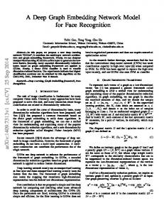
Dataset and settings. For the license plate recognition experiments, we use a dataset of 45,000 annotated license plate images obtained from the authors of [24]. The images contain segmented United States (US) plates from several states. Although license plate recognition is sometimes perceived as an easy task, for US plates the difficulty is higher since there is not a standardized system. Therefore, there exist many plate templates per state with different fonts, designs, and even containing graphical symbols or backgrounds. Moreover, the images were gathered from different sources at different times of the day, with significant illumination changes and non-optimized camera placements (e.g. angular distortions). The dataset is split into a training/test set of about 34K / 11K plates. Image features are extracted as described in Section 2.2. In our implementation, the low-level features are SIFT descriptors [11] whose dimensionality is reduced from 128 down to 32 dimensions. We use a visual vocabulary of 64 Gaussians and consider only the gradient with respect to the mean parameters. We split the word image into 4 regions (4 vertical stripes). This results into a 32 × 64 × 4=8,192-dimensional FV signature. The SPOC (with up to 5 levels) is computed for each existing label as described in Section 2.3, using as alphabet L = {0 . . . 9} ∪ {A . . . Z}. The proposed method is trained as explained in Section 2.5 with image/label pairs from the training set, and is evaluated on images from the test set, where the arg max of Eq. (2) goes over the set of unique 5K labels of the test set. Initialization was done with the random sampling explained in page 6. For evaluation we measure the accuracy vs. reject characteristic as done in [24]. For each image, we find the label with the highest value of the compatibility function F(x, y; w), and count the number of times it coincides with the ground-truth. We allow for rejection if the value of F(x, y; w) does not exceed a threshold. Baselines. We compare the proposed method against two baselines: (i) the “global” approach of [24], where recognition is based on a nearest neighbor (NN), and (ii) a bottomup approach. The latter is a state-of-the-art OCR system for recognition of US plates. Results. Fig. 2 shows the results of the comparison in two scenarios: taking into account all the labels of the test set (Fig. 2 left), and taking into account only the labels that have occurrences in the training set (Fig. 2 right). The latter allows a fair comparison to the NN approach, since it can only deal with labels seen during training, and also to verify that the proposed method generalizes well to unseen labels. First, we observe that the OCR obtains accuracies of 80-95% for moderate reject rates, which confirms that the dataset is challenging. Some of them are the presence of graphical symbols (e.g. handicapped symbol, state symbol), that are occasionally mistaken with characters. In contrast, the NN and label embedding, as they are based on global features, seem not so sensitive to these defects and obtain accuracies of 93.3% and 96.1% (at 0% reject in Fig. 2 (right)), respectively. NN does not have a mechanism for zero-shot learning and thus tends to reject unseen plates (see Fig. 2(left)). However, even in the subset of "seen" plates, label embedding has a ∼ 2% edge over NN. We observe that the proposed method does not “overfit” to the seen classes, as there is less than a 2% difference in accuracy (at 0% rejection) when considering all classes (seen+unseen) or only the seen ones.

8

RODRIGUEZ-SERRANO, PERRONNIN: LABEL EMBEDDING FOR TEXT RECOGNITION 1 0.9 0.95 Accuracy

Accuracy

0.8 0.7 0.6 0.5

Embedding ALPR 1−NN

0.4 0.3 0

0.2

0.4 0.6 Rejection

0.8

0.9

0.85

1

0.8 0

0.2

Embedding ALPR 1−NN 0.4 0.6 0.8 1 Rejection

Figure 2: License plate results. Left: using the whole test set. Right: Using only the subset of images which have a true match in the database.

We highlight that, on the one hand, the proposed approach has an unfair advantage to the OCR, since it searches in a lexicon of 5K labels while the OCR software does not have the means to specify a lexicon. On the other hand, since the OCR system is specifically designed for US plates, it is reasonable to assume that it handles prior information of the specific fonts and plate designs, and that it involves optimized pre- and post-processing steps, which is an unfair advantage over label embedding.

3.2

Scene text recognition

Dataset and settings. We perform experiments on the public IIIT-5K set [13], which is the largest existing dataset of scene text recognition with a total of 5000 cropped word images. We use the evaluation protocol of [13], with a training/test split of 2000/3000 images. The dataset is challenging, since the images contain difficulties such as variety of font, colors, designs (angled text, text in a semi-circle), and textured background. SPOC and image features are extracted as in the last subsection. One important remark is that the FV we extract does not rely on pre-processing the image with standard operations such as binarization, unlike the state-of-the-art [13]. For this experiment we did not obtain good results with the random initialization, so we apply the RR initialization (page 6), and the SGD thereafter, although it converges quickly and barely modifies the RR solution. We observed a small improvement by applying a PCA on the SPOC embeddings. The label embedding based method obtains significantly higher accuracy than the bottom-up approach for |Y| = 50 and comparable accuracy for |Y| = 1000. Baseline. For this database we compare against [13], which uses a system based on a high-order CRF built over candidate character detections, and that obtains state-of-the-art results. We do not consider the NN baseline as it is clear from the previous experiment that systems that do not offer zero-shot learning are not competitive for this task. Results are summarized in Table 2 for different values of the lexicon size. The first situation (|Y| = 50) corresponds to a word-spotting scenario as defined in [26]. The second situation (|Y| = 1000) is a moderate-vocabulary recognition task.

RODRIGUEZ-SERRANO, PERRONNIN: LABEL EMBEDDING FOR TEXT RECOGNITION

Method Mishra et al. [13] Label embedding

9

Accuracy |Y| = 50 |Y| = 1000 64.1% 57.5 % 76.1% 57.4 %

Table 2: Recognition results on the IIIT-5K dataset Table 3: Retrieval results on IIIT-5K Method Top-1 acc FV 38.0 FV+metric 42.2 DTW 37.0 Label emb 43.7

3.3

Table 4: Sample query images and top-1 match using the image similarity.

Scene text retrieval

In this experiment, we test the similarity learning approach described in Section 2.6. We maintain the IIIT-5K dataset but now consider the task of image matching: given a query image, rank the images of a database according to the lexical similarity with respect to the query. This is usually achieved by defining a similarity k(θ , θ 0 ) between images that captures the lexical similarity. In this case, to evaluate accuracy we select the subset of test images that have an image with the same label in the training set. To that end, we propose to use the method explained in Section 3, which uses a similarity function of the form k(θ , θ 0 ) = θ T Mθ 0 where M = WW T , and W is the matrix learned for the recognition task. We compare this method to : 1. The dot product between the FV image embeddings. This is an approximate explicit embedding of the Fisher kernel, which obtained state-of-the-art results in image retrieval [20]. 2. Learning M explicitly with a similarity learning algorithm. We use SSI [1], as its objective function shares some similarities and it also uses SGD. 3. The similarity computed by dynamic time warping on sequences of local gradient histogram features, which is state-of-the-art in image-based word-spotting [23]. We measure the top-1 accuracy, i.e. fraction of the test set where the top-1 retrieved element is correct. Results are shown in table 3. Table 4 illustrates visual results. We observe that learning a metric with SSI improves over the FV and DTW baselines, but that the metric learned by label embedding provides higher accuracy. In other words, the projection W matrix obtained by the proposed text recognition method is a good projection for images themselves. An advantage of this approach is that, unlike SSI [1], the label embedding does not require the training set to contain pairs of images with the same labels, thus typically smaller sets are needed.

4

Conclusions

We have proposed a new approach for text recognition where images and words from a lexicon are explicitly embedded in a common space, and recognition proceeds by finding the closest label given an image. The method works thanks to the SPOC representation and a

10 RODRIGUEZ-SERRANO, PERRONNIN: LABEL EMBEDDING FOR TEXT RECOGNITION

relaxed structured learning algorithm to find the optimal space. The method does not attempt to find characters in the word, does not require dedicated pre-processing of the image and is efficient at runtime, yet its accuracy is competitive with the traditional bottom-up approaches in various scene text scenarios. We show positive results for lexicons of up to 1K/5K examples. The challenge now is to make the method scale to large lexicons. We believe that, as such a system will need to distinguish between finegrained words, it will require far more than the 2000 training samples available in the IIIT-5K set. Since we use a retrieval-based approach for text recognition, there is abundant literature on large-scale retrieval that can be leveraged for this task, for example on compressing histogram descriptors [5].

References [1] B. Bai, J. Weston, D. Grangier, R. Collobert, O. Chapelle, and K. Weinberger. Supervised semantic indexing. In CIKM, 2009. [2] K. Chatfield, V. Lempitsky, A. Vedaldi, and A. Zisserman. The devil is in the details: an evaluation of recent feature encoding methods. In BMVC, 2011. [3] G. Csurka, C. Dance, L Fan, J. Willamowski, and C. Bray. Visual categorization with bags of keypoints. In ECCV SLCV workshop, 2004. [4] Raman Jain and CV Jawahar. Towards more effective distance functions for word image matching. In DAS, pages 363–370. ACM, 2010. [5] Hervé Jégou, Florent Perronnin, Matthijs Douze, Jorge Sánchez, Patrick Pérez, and Cordelia Schmid. Aggregating local image descriptors into compact codes. IEEE Trans. Pattern Anal. Mach. Intell., 34(9), 2012. [6] T. Joachims. Optimizing search engines using clickthrough data. In SIGKDD, 2002. [7] Hugo Larochelle, Dumitru Erhan, and Yoshua Bengio. Zero-data learning of new tasks. In AAAI, 2008. [8] S. Lazebnik, C. Schmid, and J. Ponce. Beyond bags of features: Spatial pyramid matching for recognizing natural scene categories. In CVPR, 2006. [9] Y. LeCun, L. Bottou, G. Orr, and K. Muller. Efficient backprop. In G. Orr and Muller K., editors, Neural Networks: Tricks of the trade. Springer, 1998. [10] Huma Lodhi, Craig Saunders, John Shawe-Taylor, Nello Cristianini, and Chris Watkins. Text classification using string kernels. J. Mach. Learn. Res., 2, 2002. [11] D. Lowe. Distinctive image features from scale-invariant keypoints. IJCV, 60(2), 2004. [12] Thomas Mensink, Jakob Verbeek, Florent Perronnin, and Gabriela Csurka. Metric Learning for Large Scale Image Classification: Generalizing to New Classes at NearZero Cost. In ECCV, 2012. [13] A. Mishra, K. Alahari, and C. V. Jawahar. Scene text recognition using higher order language priors. In BMVC, 2012.

RODRIGUEZ-SERRANO, PERRONNIN: LABEL EMBEDDING FOR TEXT RECOGNITION 11

[14] A. Mishra, K. Alahari, and C. V. Jawahar. Top-down and bottom-up cues for scene text recognition. In CVPR, 2012. [15] Lukas Neumann and Jiri Matas. Real-time scene text localization and recognition. In CVPR, 2012. [16] Tatiana Novikova, Olga Barinova, Pushmeet Kohli, and Victor Lempitsky. Largelexicon attribute-consistent text recognition in natural images. In ECCV, 2012. [17] S. Nowozin and C. Lampert. Structured learning and prediction in computer vision. Foundations and Trends in Computer Graphics and Vision, 2011. [18] F. Perronnin, J. Sánchez, and Y. Liu. Large-scale image categorization with explicit data embedding. In CVPR, 2010. [19] F. Perronnin, J. Sánchez, and Thomas Mensink. Improving the Fisher kernel for largescale image classification. In ECCV, 2010. [20] Florent Perronnin, Yan Liu, Jorge Sánchez, and Herve Poirier. Large-scale image retrieval with compressed Fisher vectors. In CVPR, 2010. [21] Toni M Rath and Raghavan Manmatha. Word image matching using dynamic time warping. In CVPR, 2003. [22] Jose Rodriguez-Serrano and Florent Perronnin. A model-based sequence similarity with application to handwritten word spotting. IEEE Trans. PAMI, 34(11), 2012. [23] José A. Rodríguez-Serrano and Florent Perronnin. A model-based sequence similarity with application to handwritten word spotting. IEEE Trans. PAMI, 34(11), 2012. [24] José A. Rodríguez-Serrano, Harsimrat Sandhawalia, Raja Bala, Florent Perronnin, and Craig Saunders. Data-driven vehicle identification by image matching. In ECCV Workshop on Computer Vision for Vehicle Technology, 2012. [25] B. Schölkopf, A. Smola, and K.-R. Müller. Non-linear component analysis as a kernel eigenvalue problem. In Neural Computation, 1998. [26] Kai Wang and Serge Belongie. Word spotting in the wild. In ECCV, 2010. [27] Kai Wang, Boris Babenko, and Serge Belongie. End-to-end scene text recognition. In ICCV, 2011. [28] Jason Weston, Samy Bengio, and Nicolas Usunier. Large scale image annotation: Learning to rank with joint word-image embeddings. ECML, 2010. [29] C. Williams and M. Seeger. Using the Nyström method to speed up kernel machines. In NIPS, 2001.