PHYSICS OF FLUIDS
VOLUME 13, NUMBER 10
OCTOBER 2001
Lagrangian approaches for particle collisions: The colliding particle velocity correlation in the multiple particles tracking method and in the stochastic approach A. Berlemont,a) P. Achim, and Z. Chang UMR 6614-CORIA Technopoˆle du Madrillet BP 12, 76801 Saint-Etienne-du-Rouvray Cedex, France
共Received 13 December 1999; accepted 20 June 2001兲 Two different Lagrangian approaches for particle/particle collisions are described. The first model is based on the simultaneous tracking of several particles and suitable treatment is developed on particle pairs to detect collisions on each time step of the particle trajectory realization. The second method is based on a stochastic approach where one single particle is tracked, and successive random processes are applied to generate a fictitious partner of collision. In order to validate both approaches, simulations have been carried out in homogeneous isotropic turbulence and they have been compared with LES data. The particle/particle correlated motion through the surrounding fluid is proved to be a key parameter in a particle/particle collision process. © 2001 American Institute of Physics. 关DOI: 10.1063/1.1396845兴
I. INTRODUCTION
In the stochastic approach for particle collisions, a collision probability is defined and a random process is first used to decide if a collision occurs. Several successive random processes are then involved in order to characterize the collision particle partner in terms of velocity, concentration, impact location, or diameter when polydispersed particles are considered. In the multiple particle method, several particles are simultaneously followed, and all particle pairs are examined on each time step of the particle trajectory construction in order to know if any of them are colliding. As far as the number of simultaneous trajectories is limited, simulations are carried out on several launches of a given number of particles. They are initially randomly distributed in a box whose size is fixed by the desired mean distance between particle centers deduced from the initial concentration and the geometry of the case under study. The multiple particle method thus obviously appears much more time consuming. In order to validate these approaches, extensive comparisons have been carried out with LES calculations from Lavieville7 for isotropic turbulence. We thus found that an important parameter requires particular attention in our approaches, namely, the overall 共referring on the two colliding particles兲 particle/particle velocity correlation that is induced by the surrounding fluid. We first recall the Lagrangian scheme for particle tracking; we then describe the two schemes for the particle collisions in the multiple particles tracking and in the stochastic approach. Analyzing a first set of results leads us to improve the collision schemes by introducing in both methods the particle/particle correlated motion that is extensively presented. The obtained results are then compared with LES data and they are discussed.
Previous studies on Lagrangian approach for particle dispersion in turbulent fields have been developed from the simplest case of one-way coupling to more complicated problems involving two-way coupling with heat, mass, momentum, and energy exchanges between phases 共Berlemont et al.1,2兲. It appears that the development of numerical simulations of particle two-phase flows is now more and more focused on particle/particle interactions. This is a four-way coupling problem that is still unsolved in its full generality, but that was the object of much effort in recent years. Different approaches have been recently proposed and are still currently studied, leading to very encouraging results and, in some cases, to definite ones. Among these studies we find the following. 共i兲 The direct numerical simulation of both the fluid flow and the tracking of the embedded particles 共Mei et al.,3 Wang et al.,4 Zhou et al.,5 Lavieville et al.6,7兲, giving insights on underlying physical phenomena and providing us with a database for the model validation. 共ii兲 An Eulerian approach in which collisions between particles are described by using a kinetic theory approach 共Simonin et al.,8 Lavieville7兲. 共iii兲 A Lagrangian simulation based on the tracking of several particles simultaneously 共Tanaka et al.,9 Chang,10 Berlemont et al.11兲. 共iv兲 A Lagrangian simulation based on a single-particle tracking with stochastic process for collisions 共Oesterle´ and Petitjean,12 Sommerfeld,13 Berlemont and Achim14兲. In the present paper we are concerned with the third and fourth approach, which will be described and then compared with LES results from Lavieville.7 a兲
Electronic mail:
[email protected]
1070-6631/2001/13(10)/2946/11/$18.00
2946
© 2001 American Institute of Physics
Downloaded 29 Nov 2001 to 128.205.153.49. Redistribution subject to AIP license or copyright, see http://ojps.aip.org/phf/phfcr.jsp
Phys. Fluids, Vol. 13, No. 10, October 2001
Collision velocity correlation in Lagrangian approach
II. LAGRANGIAN APPROACH A. Fluid particle
Whatever the chosen Lagrangian method, the main problem, in turbulent flows, is to know the fluid instantaneous velocity field at the discrete particle location, all along the trajectory of the tracked discrete particle. Obviously, this problem is crucial because, due to various effects such as inertia and gravity, discrete particle trajectories and fluid particle trajectories do not coincide. However, fluid particle trajectories may be viewed as reference trajectories and, in any case, we have to predict them. The equation for such a prediction is very simple, due to the fact that a fluid particle 共or a discrete particle exhibiting special properties such as being nonbuoyant and/or having a vanishing diameter兲 instantaneously follows the surrounding velocity field. Therefore, we have x i 共 t⫹⌬t 兲 ⫽x i 共 t 兲 ⫹U i ⌬t,
共1兲
in which x i (t) is the location of the fluid particle at time t, U i is the instantaneous fluid velocity, and ⌬t is an increment of time, small enough so that U i is essentially constant during ⌬t. The instantaneous velocity U i is equal to the mean velocity that is known 共for instance, from turbulence model predictions兲 plus a fluctuation u i , which is unknown. We, however, know the variances of each component of u i 共again from the turbulence model predictions兲 and we may assume, for simplicity, that u i satisfies a Gaussian probability density function. But this is not enough to toss a value of the fluctuation u i since it has also to satisfy the Lagrangian velocity correlation coefficient R f L along the fluid trajectory.
larly separated by the increment ⌬t, and complying with the chosen Lagrangian correlation. The chosen Lagrangian correlation function is rewritten under the form of a matrix A 共the correlation matrix兲, which is symmetric and definite positive. Matrix components are velocity correlation at times i⌬t and j⌬t. From matrix A, we may deduce uniquely another matrix B by invoking a so-called Cholesky factorization. A vector Y with uncorrelated, centered, unit variance components is first randomly generated. One then shows that U⫽BY . As time is evolving the matrix is growing, but we limit the maximum correlation time, for example, it is assumed that the Lagrangian correlation function is equal to zero for a time gap greater than five times the fluid Lagrangian time scale L . When the time step is L/5, the size of matrix A is 共25, 25兲 in the one-dimensional 共1-D兲 case. Originally designed for 1-D dispersion, the procedure has been after generalized to the 2-D and 3-D cases. Details may be found elsewhere 共Berlemont et al.,1 Gouesbet et al.15兲. The Lagrangian correlation function is expressed through any kind of relation, such as Frenkiel16 or Sawford17 functions. In the present paper, the Frenkiel relation with loop parameter m⫽1 has been used:
冑
Our aim is to generate a vector U whose components are velocity fluctuations along the trajectory, at time steps regu-
冑
u i 共 t⫹⌬t 兲 u i 共 t 兲 ⫽ u 2i 共 t⫹⌬t 兲 u 2i 共 t 兲 exp ⫻cos
冉
m⌬t 共 m ⫹1 兲 Li 2
u i 共 t⫹⌬t 兲 u j 共 t 兲 ⫽u i 共 t 兲 u j 共 t 兲 exp
B. Correlation matrix
We account for the fact that R f L is actually a predominant quantity, at least conceptually, and we take it as input. More important, the procedure is designed in such a way that any R f L shape may be a priori chosen and introduced in the code. The stochastic process is then slaved to the chosen correlation. The slaving process satisfies the following properties. 共i兲 The probability density function of the velocity fluctuations is assumed to be normal. This assumption may, in principle, be relaxed, allowing possibly testing the influence of pdfs on diffusion 共or dispersion兲. For predictions in turbulent flows, the relaxation of this assumption would require knowledge of the actual pdf. The accuracy with which this pdf should be known depends on the sensitivity of particle behavior to it. Up to now, this issue has not been studied, but the interest of such a study is warranted. 共ii兲 The stochastic process must reproduce one point correlation of velocity fluctuations, known from the turbulence model 共or from experiments兲. 共iii兲 Finally, this stochastic process must also correctly reproduce the fluid particle Lagrangian correlation function of velocities along the trajectory, according to the chosen shape of R f L .
2947
⫻cos
冉
冉
冊
冉
⫺⌬t 共 m ⫹1 兲 Li 2
共2兲
,
⫺⌬t 共 m 2 ⫹1 兲 Li j
冊
冊
m⌬t , 共 m ⫹1 兲 Li j 2
冊
共3兲
where
Li ⫽C Li
u 2i 共 t 兲
⑀
and
with C Li ⫽0.2
Li j ⫽C Li j and
兩 u i共 t 兲 u j共 t 兲兩 , ⑀
C Li j ⫽1.
共4兲
A discussion on the chosen expression for the Lagrangian time correlation can be found in Gouesbet et al.,15 but note that the main advantage of the above scheme is not the Frenkiel correlation but the ability of the method to satisfy any given fluctuating velocity correlation. C. Discrete particle
The above scheme has been set up for fluid particle trajectories, but the main interest in two-phase flow modeling remains the characterization of the discrete phase behavior. For a discrete particle, the forces acting on the particle are expressed through the Maxey and Riley18 equation; a discrete particle trajectory is obtained by integrating its equation of motion, which in the presented cases reduces to drag and gravity terms, as the ratio of particle density to fluid density is quite large 共25–200兲:
Downloaded 29 Nov 2001 to 128.205.153.49. Redistribution subject to AIP license or copyright, see http://ojps.aip.org/phf/phfcr.jsp
2948
Phys. Fluids, Vol. 13, No. 10, October 2001
Berlemont, Achim, and Chang
L Eii ⫽C i Lii
FIG. 1. The pilot fluid particle and the discrete particle.
p
dV 3 f ⫽⫺ C 共 V⫺U兲 兩 V⫺U兩 ⫹ 共 p ⫺ f 兲 g, dt 4 d D
共5兲
where C D⫽
24 兲, 共 1⫹0.15 Re0.687 p Rep
Rep ⫽
兩 V⫺U兩 d .
共6兲
Here Rep is the particle Reynolds number, which is assumed to be smaller than 200, V and U are the particle and fluid velocity vectors, respectively, and g is the gravity vector. In addition, p and f are the particle and fluid density, respectively, d is the particle diameter, and is the fluid cinematic viscosity. The main problem in the equation of motion is that the fluid velocity is the velocity on the discrete particle location. To guess that velocity, a pilot fluid particle is simultaneously followed with the discrete particle using the above-described method, and the fluid velocity is transferred from the fluid particle location to the discrete particle location by the use of an Eulerian correlation 共Fig. 1兲. These correlations are expressed in a coordinate system, where the first unit vector is colinear to the vector between the fluid and particle locations, respectively. In the random process for the spatial correlation, we assume that uជ P ⫽ 兵 ␥ 其 uជ F ⫹ 兵 其 yជ ,
共7兲
where uជ P and uជ F are the fluid fluctuating velocity vector on the particle location P and on the fluid location F, respectively. Here yជ is a vector with uncorrelated, centered, unit variance components. It has been found 共Chang10兲 that T
兵 ␥ 其 ⫽uជ P uជ F uជ F uជ F
T ⫺1
T
T
兵 其兵 其 T ⫽uជ F uជ P ⫺ 兵 ␥ 其 uជ F uជ F 兵 ␥ 其 T .
共8兲
The required spatial correlation can be expressed through Frenkiel relations:
冑 u 冑u F2 i
u Fi u Pj ⫽u Fi u Fj exp
P2 i
冉
F2 i
exp
冉
⫺r 共 n 2 ⫹1 兲 L Eii
⫺r 共 n 2 ⫹1 兲 L Ei j
冊 冉 cos
冊 冉 cos
nr 共 n 2 ⫹1 兲 L Eii
nr 共 n 2 ⫹1 兲 L Ei j
冊
,
冊
, 共9兲
共10兲
where r is the distance between F and P, n is equal to 1, and the fluid Eulerian length scales can be estimated by
冑
L Ei j ⫽C i j Li j 兩 u Fi u Fj 兩 ,
and
共11兲
where the constants C 1 and C i j are fixed to 1 and C 2 ⫽C 3 ⫽C 1 /2 for isotropic turbulence or when no information can be used from experimental data. The fluid particle is followed on several time steps, until the distance r is larger than a given length scale L D 共the mean value of the Eulerian scales兲 that is characterizing a correlation domain around the fluid particle 共Fig. 1兲. A new fluid particle is then considered and the process is repeated. This scheme is intending to simulate the crossing trajectory effects in a very physical way. However, that scheme has been modified in the multiple particles tracking approach in order to get less time consuming and less memory storage. As several particles, namely 300 or 500, are simultaneously followed, the same number of correlation matrices are involved, which requires quite large computing facilities. Thus a one step scheme has been set up, which is defined in the same way as the above method, but considering only one time step drastically reduces the correlation matrix. No matrix is then necessary, since algebraic relations are obtained to guess the fluid velocities. This degenerated scheme is quite similar to the method, which is described by Burry and Bergeles,19 but it does not allow to choose the R f L shape, which is directly generated by the process itself as an exponential decrease.
III. PARTICLE COLLISIONS A. The stochastic collision model
We first consider a one-particle Lagrangian approach. We thus have to use a stochastic particle/particle collision model, as described by Sommerfeld,13 which is driven through a collision frequency. By assuming that the fluctuating motion of the discrete phase is analogous to the thermal motion of molecules in gas, the kinetic theory formalism can help to derive an expression for the collision frequency. Let us consider two particle classes, which are identified through the diameters d 1 and d 2 共radius r 1 and r 2 兲, the instantaneous ជ 1 and Vជ 2 , and the number of particles per unit of velocities V volume N p1 and N p2 . The collision frequency for the particle 1 to collide with particle 2 is
f coll⫽ 共 d 1 ⫹d 2 兲 2 N p2 4
and
u Fi u iP ⫽
冑u
冕冕
⫹⬁
⫺⬁
ជ rel兩 f 共p2 兲 d vជ 1 d vជ 2 , 兩V
共12兲
where
ជ rel兩 ⫽ 兩 Vជ 2 ⫺Vជ 1 兩 . 兩V
共13兲
The most important term in the above equation is the particle/particle pair distribution function f (2) p . When assuming that colliding particle velocities are independent 共molecular chaos assumption兲, each particle velocity is satisfying a Gaussian distribution f (1) p : f 共p1 兲 ⫽
1 共 2 v 2p 兲 3/2
冉 冊
exp ⫺
ជ V 2p
2 v 2p
,
共14兲
Downloaded 29 Nov 2001 to 128.205.153.49. Redistribution subject to AIP license or copyright, see http://ojps.aip.org/phf/phfcr.jsp
Phys. Fluids, Vol. 13, No. 10, October 2001
Collision velocity correlation in Lagrangian approach
2949
FIG. 2. Collision coordinate system.
and the particle/particle pair distribution function is the product of the two distribution functions. The collision frequency then reads 共Abrahamson20 and Gourdel21兲 as
f coll⫽ 共 d 1 ⫹d 2 兲 2 N p2 储 ¯V rel储 H 共 z 兲 , 4
共15兲
with H共 z 兲⫽
exp共 ⫺z 兲
冑 z
冉 冊
⫹erf共 冑z 兲 1⫹
1
2z
,
z⫽
1 储 ¯V rel储 2
. 2 v 2⫹ v 2 1 2 共16兲
It thus appears that the variable z represents the ratio between the particle relative mean velocity and the particle turbulent fluctuating motions. Two asymptotic behaviors are then derived, namely for large values of z and for small values of z. For large values of z 共the high drift between particles兲, H(z) tends toward 1, and thus f coll⫽
N 共 d ⫹d 2 兲 2 储 V 1 ⫺V 2 储 , 4 p2 1
共17兲
and the collision frequency is thus depending essentially on particle mean relative velocity. For small values of z 共the small drift between particles兲, using a Taylor expansion for H(z), leads to 2 3/2
f coll⫽
1/2
4
冑
N p2 共 d 1 ⫹d 2 兲 2 v 21 ⫹ v 22 ,
共18兲
which means that the collision frequency mainly depends on the particle agitation. The collision probability p 12 of particle 1 to collide with particle 2 then reads as p 12⫽ f coll⌬t,
共19兲
where the time step ⌬t is assumed to be small enough 共of the order of c /10, where c ⫽1/f coll兲. To decide whether there is a collision or not, a uniform random number 共between 0 and 1兲 is tossed and the collision occurs when it is smaller than the collision probability. When a collision is detected, the problem is then to describe the particle interactions. In the present work, binary perfectly elastic collisions are only considered. When two particles are colliding, the problem is first to determine the points on the particle surfaces, which are in contact. We thus
move to a coordinate system (Ox⬘ y⬘ z⬘ ) where the main axis ជ rel direction and O is the center of the (Ox⬘ ) is in the V tracked particle 关Fig. 2共a兲兴. A uniform random number  between 0 and 1 is used to obtain the normalized impact parameter b 关 b⫽B/(r 1 ⫹r 2 ) ⫽ 冑 兴 and another uniform random number is then tossed to get the ␣ angle, with 0⭐ ␣ ⭐2 关Fig. 2共b兲兴. We then move to the new coordinate system (Ox⬙ y⬙ z⬙ ) such as the Ox⬙ axis is on the particle center direction 关Fig. 2共c兲兴. Here, ⌿ and ⌽ angles are defined by ⌿⫽arctan
冉
b sin ␣
冑1⫺b
2
sin ␣ 2
冊
⌽⫽arctan
,
冉
⫺b cos ␣
冑1⫺b 2
冊
.
共20兲
As the proposed test case is concerning identical particles and binary collisions without rotation, the collision process is then quite simple. Using subscript ‘‘ac’’ for velocities after collision, we get 共 V 1 x 兲 ac⫺ 共 V 2 x 兲 ac⫽⫺k 共 V 1 x 兲 , ⬙
⬙
⬙
共 V 1 y 兲 ac⫽V 1 y , ⬙
共 V 2 y 兲 ac⫽V 2 y ,
共 V 1 z 兲 ac⫽V 1 z ,
共 V 2 z 兲 ac⫽V 2 z ,
⬙
⬙
⬙
⬙
⬙
⬙
共21兲
⬙
where k is the restitution coefficient 共⫽1 for perfectly elastic collisions兲. As we consider identical particles 共with mass m p 兲, the particle impulsion reads as J 1 ⫽⫺ 共 1⫹k 兲
mp 共 V 1 x ⫺V 2 x 兲 , ⬙ ⬙ 2
which leads to 共 V 1 x 兲 ac⫽V 1 x ⫹
J1 1⫹k ⫽V 1 x ⫺ 共 V 1 x ⫺V 2 x 兲 , ⬙ ⬙ ⬙ mp 2
共 V 2 x 兲 ac⫽V 2 x ⫺
J1 1⫹k ⫽V 2 x ⫹ 共 V 1 x ⫺V 2 x 兲 . ⬙ ⬙ ⬙ mp 2
⬙
⬙
⬙
⬙
共22兲
B. The multiple particles collision model
In the multiple particles Lagrangian tracking approach 共Chang,10 Berlemont et al.11兲, several particles are simultaneously followed, and suitable treatment is developed on
Downloaded 29 Nov 2001 to 128.205.153.49. Redistribution subject to AIP license or copyright, see http://ojps.aip.org/phf/phfcr.jsp
2950
Phys. Fluids, Vol. 13, No. 10, October 2001
particle pairs for collisions 共only binary collisions are considered兲, at each time step of the particle trajectories construction. To comply with the specific conditions of the test case under study, we have to both keep a constant concentration and to estimate the particle turbulent dispersion for a given time of tracking. As far as the number of simultaneous trajectories is limited, simulations are carried out on 1000 successive launches of 500 particles. Thus, a 3-D box is defined where the particles are initially randomly distributed, and the box size is fixed by the desired void fraction. A periodic boundary condition is applied to the dispersed phase: particles that are moving outside the box are reinjected on the opposite side of the box. Note that the calculation process is integrating the particle box to box motion. After moving the 500 particles, we determine all the colliding particles 共when the distance between their centers is smaller than the sum of their radius兲. When a collision occurs, a change of the coordinate system is carried out in order to determine the particle velocities after the collision. In the new reference frame, the first coordinate vector is aligned with the particle centers and the above process for the particle velocities after collision is used in the same way as for the stochastic approach.
IV. COMPARISONS WITH LES RESULTS
Simulations have been carried out by Lavieville7 to describe the 3-D particle behavior in isotropic turbulence, without gravity, in order to enhance the influence of the particle/ particle correlated motion in the collision process. In the frame of the large eddy simulation approach, the instantaneous turbulent fluid velocity is decomposed into a large eddy field 共the resolved field兲 and a small scale turbulent field 共the residual or subgrid field兲. In Lavieville’s study25 the diffusive effect of the residual field is modeled with a subgrid eddy viscosity proposed by Smagorinsky,22 completed by the scale similarity closure assumption proposed by Bardina23 to represent the contribution of the subgrid scale turbulence to the transport of the large eddy field. Simulation data, which are input in our calculations, are given below: Fluid: Density: f ⫽1.17 kg/m3 ; cinematic viscosity: ⫽1.47⫻10⫺5 m2/s; mean velocities: U x ⫽U y ⫽U z ⫽0; fluctuating velocities: u 2x ⫽u 2y ⫽u z2 ⫽8.76⫻10⫺2 m2/s2; Lagrangian integral time scale: L⫽26.⫻10⫺3 s; Eulerian length
冑
scales: L E11⫽ L u 2x ⫽7.8⫻10⫺3 m; and L E22⫽L E33 ⫽L E11/2⫽3.9⫻10⫺3 m. Particles: Diameter: d⫽656 m; density: p ⫽25, 50, 100, and 200 kg/m3. The choice of particle diameter in the Lavieville7 study is the smallest accessible one according to the computer resources used by his collision algorithm, which leads to a (338) 3 grid. The particle diameter thus appears to be greater than the Kolmogorov scale (0.15⫻10⫺3 m), but it remains smaller than the Taylor microscale (2⫻10⫺3 m). All the calculations have been carried out with the assumption that Eq. 共5兲 is still valid for the particle equation of motion and no specific study has been devoted to the possible influence of
Berlemont, Achim, and Chang TABLE I. Particle kinetic energy without collisions.
p 共kg/m3兲 k p 共m /s 兲 2 2
LES Matrix One step
25
50
100
200
0.071 0.070 0.075
0.053 0.052 0.054
0.037 0.037 0.036
0.023 0.024 0.022
the Saffman effect or the nonuniform pressure gradient over the sphere. The Stokes number based on the particle relaxation time and the Kolmogorov time scale is at least 12 and the Stokes number based on the fluid integral time scale is in between 1 and 5. Thus, the clustering of particles does not seem to have a noticeable influence on the collision process. Note that in our Lagrangian calculations no effect of preferential concentration of the particles are involved. Particle mean velocities and fluctuating velocities are set equal to the fluid values at injection, but particles are allowed to disperse sufficiently to be statistically in equilibrium with the fluid turbulence before any calculation of the statistics. Moreover, collisions are introduced in the simulations when the particles have reached steady state without collisions. Simulations without collisions show a decrease of the particle kinetic energy (k p ⫽0.5v 2ii ) toward asymptotic values. As expected, these values are smaller when the particle density is increasing 共leading to an increase of the particle relaxation time兲. However, the initial value of the fluid integral time scale from LES leads to too small asymptotic values of the particle fluctuating motion. Such behavior has been yet observed by Chang10 and Sommerfeld24 and is mainly linked to the Eulerian step in the particle-tracking scheme. But it appears quite difficult to suppress that step since it is intended to describe the crossing trajectory effects. To overcome that problem one can think to make the Eulerian step depending only on the mean relative velocity between the fluid and the particles. Thus, the difference between the fluid and particle fluctuating motion is no more contributing to any decorrelation between the two trajectories. We have tried that scheme and the results are in very good agreement with the LES results. However, no rigorous theoretical statement has been found to justify that scheme. Thus, it has not been used in the following. In order to fit our simulations with LES results when no collisions are included, the fluid integral time scale has then been increased, namely L⫽52.⫻10⫺3 s for the correlation matrix method and L⫽38.⫻10⫺3 s for the one-step method. We then notice in Table I the good agreement between LES results and the simulations. As mentioned above, the reason for two different L values is linked to the Eulerian step. Its influence in the one-step method is less important than in the matrix approach since no Eulerian correlation scale (L D ) is involved in the one-step method: the fluid particle is moved to the discrete particle location on each time step, when several fluid velocity transfers can occur in the matrix scheme. We then report in Table II the comparisons for the particle kinetic energy k p between our simulation with both approaches and LES results, for two different particle densities, namely p ⫽50 and 100 kg m⫺3, and various particle volu-
Downloaded 29 Nov 2001 to 128.205.153.49. Redistribution subject to AIP license or copyright, see http://ojps.aip.org/phf/phfcr.jsp
Phys. Fluids, Vol. 13, No. 10, October 2001
Collision velocity correlation in Lagrangian approach
metric fractions ␣ 2 . As we previously observed with the multiple particles Lagrangian tracking and as Sommerfeld24 also noticed with his stochastic approach, a decrease of the particle energy is obtained when collisions are included in the simulations, which is not observed in the LES simulations 共Lavieville et al.25兲. It thus appears that the particle motion was insufficiently correlated to the fluid motion, due to collisions. It was deduced that during the collision process the fluid/particle correlation u p u f was partially destroyed, in both approaches but not in the same way. Each approach has thus been modified to account for the correlation between the fluctuating motion of the colliding particles through the surrounding fluid. V. FLUIDÕPARTICLE CORRELATION A. The stochastic collision model
Such a relation is improving the results but, as noticed by the author, the real value of c corr remains quite empirical. Our approach is quite different and it is now described. As mentioned above, the collision frequency is deduced from the kinetic theory and is linked to the particle/particle pair distribution function. But the molecular chaos assumption can be no more valid when the distance between the two particles is small, leading to a possible correlation between their velocities through the turbulent eddy in which they are moving. We then have to introduce a distribution function f (2) p , which accounts for the fact that the two particles are driven by the same fluid. This important point has been first stated and solved by Lavieville et al.6 for two identical particles. Pigeonneau26 recently proposed an extension of that study to particles with different diameters. Here f (2) p is written under the following relation:
In order to overcome this problem, Sommerfeld24 has recently proposed to correlate the fictitious particle velocities with those of the real particle through the following relation: v 2,i ⫽R 共 p , L兲v 1,i ⫹ i 冑1⫺R 共 p , L兲 2 ,
f 共p2 兲 ⫽A 共 r 1 ,r 2 ,d 12兲 exp⫺
共23兲
where i is the rms value of the velocity component i, is a Gaussian random number, p is the particle relaxation time, and R( p , L) is given by
冉
R 共 p , L兲 ⫽exp ⫺
A 共 r 1 ,r 2 ,d 12兲 ⫽
冊
p . c corr L
共24兲
T
⫺
冑共 2 v 21 2 v 22 兲 3关 1⫺ 2f 1 2f 2 f 共 d 12兲 2 兴关 1⫺ 2f 1 2f 2 g 共 d 12兲 2 兴
1
r ir j 2 d 12
冉
冑v 21 冑v 22
100
ជ v 2 B2ជ v2 2 v 22 共25兲
,
r ir j 2 d 12
冊
⫹
共26兲
B 12,i j ⫽ f 1 f 2
1
⫹
1⫺ 2f 1 2f 2 g 共 d 12兲 2
␣ 2 (%) No collision 0.88 1.76 4.40 No collision 0.49 0.99 2.47
冋
f 共 d 12兲 2 2 1⫺ f 1 f 2 f 共 d 12兲 2
冉
r ir j 2 d 12
g 共 d 12兲 r ir j ␦ ⫺ 2 1⫺ 2f 1 2f 2 g 共 d 12兲 2 i j d 12
冊册
,
共28兲
with 共27兲
,
2f ␣ ⫽
1
LES
Multiple particles
Stochastic approach
0.053 0.055 0.056 0.059 0.037 0.038 0.039 0.041
0.054 0.053 0.045 0.038 0.036 0.034 0.032 0.028
0.052 0.043 0.040 0.039 0.037 0.032 0.030 0.029
共29兲
1⫹ p ␣ / L*␣
and
50
2 v 21
T
⫹
,
TABLE II. Particle kinetic energy with collisions: uncorrelated models.
p 共kg m⫺3兲
冊
ជ v 1 B1ជ v1
1
1⫺ 2f 1 2f 2 f 共 d 12兲 2 ⫻ ␦i j⫺
ជ v 1 B12ជ v2
冉
T
where
B ␣ 共␣ ⫽1 or 2兲 and B 12 are the correlation matrices whose elements are defined by B ␣ ,i j ⫽
2951
冉
f 共 d 12兲 ⫽exp ⫺
冉
g 共 d 12兲 ⫽ 1⫺
冊 冊 冉
d 12 , LE11
冊
d 12 d 12 exp ⫺ ; 2L E11 L E11
共30兲
d 12 is the distance between the two particles, and L* is the fluid integral time scale along the particle path and ␣ identifies the two particles. In the presented study we are not in the Saffman–Turner limit case of vanishing particle inertia, and the particles are
Downloaded 29 Nov 2001 to 128.205.153.49. Redistribution subject to AIP license or copyright, see http://ojps.aip.org/phf/phfcr.jsp
2952
Phys. Fluids, Vol. 13, No. 10, October 2001
Berlemont, Achim, and Chang
FIG. 3. Relative velocity of colliding particles: p ⫽200 kg m⫺3.
FIG. 4. Relative velocity of colliding particles: p ⫽25 kg m⫺3.
much more influenced by quite large turbulence scales than small scales. But note that the relations for f (d 12) and g(d 12) should be replaced by relations that satisfy the condition f (r)⫽1⫺r 2 /2 T2 ⫹O(r 3 ) for small r 共such as Sawford17 relations兲 in order to recover the Saffman–Turner limit case result. The last unknown is L* which is defined and calculated by
Our calculations showed that when p / L* is greater than 20, the variation of the collision frequency is less than 5% between the correlated model and the uncorrelated model. The calculations with the stochastic correlated model that are presented in the next sections are carried out by using relation 共32兲 for in the collision frequency expression and by tossing the velocity of the collision partner with respect to relation 共25兲.
L* ⫽
1 3
冕
⬁
u pf i 共 t 兲 u Pf i 共 t⫹ 兲
0
u P2 fi 共t兲
d,
共31兲
where the superscript P refers to the discrete particle location. We can notice that the above relations lead to statistical independence of the colliding particle velocities when the distance d 12 between the particles is increased, as the functions f (d 12) and g(d 12) tend toward 0. Developing relation 共12兲 then leads to a new expression for the collision frequency that still reads as relations 共14兲 and 共15兲, but the variable z is now defined by z⫽
1 储 ¯V rel储 2 , 2 2p
with
冑
2p ⫽ v 21 ⫹ v 22 ⫺2 v 21 v 22 f 1 f 2 f 共 d 12兲 .
共32兲
In order to illustrate the particle/particle pair distribution function influence we present in Figs. 3 and 4 the relative velocity distribution function for two colliding particles, for p ⫽200 kg/m3 and p ⫽25 kg/m3, for two arbitrary collision angles. As we are here concerned with 3-D simulations, we first observe that the relative velocity distribution functions are centered on nonzero values. For p ⫽200 kg/m3, due to the quite large particle relaxation time 共 p ⫽280 ms, p / L* ⫽7.8兲 when compared with the fluid time scale, the influence of the correlated model on the results is very slight. Conversely, for p ⫽25 kg/m3 共 p ⫽65 ms, p / L* ⫽1.5兲, a quite important effect is noticed, and the agreement with LES simulations is highly improved.
B. The multiple particles collision model
When a collision occurs between a particle pair, both particle velocities are modified. Each discrete particle is followed with its own fluid particle, without any correlation between the two fluid motions, even when they are on the same location. As a consequence modifying the particle velocities during a collision is introducing a decorrelation between the discrete particle and the fluid particle on each trajectory. That behavior has been proved erroneous by LES simulations, as the overall 共that means the sum on the two colliding particles兲 correlation u p u f remains constant during the collision. As the discrete particle velocities are fully determined through the collision process, we decided to modify each associated fluid velocity in order to respect the u p u f invariance before and after the collision. In the previously defined coordinate system for the collision process, we write 共 V 1x ⬙ 兲 ac共 U 1x ⬙ 兲 ac⫹ 共 V 2x ⬙ 兲 ac共 U 2x ⬙ 兲 ac
⫽V 1x ⬙ U 1x ⬙ ⫹V 2x ⬙ U 2x ⬙ .
共33兲
To determine the fluid velocities (U 1x ⬙ ) ac and (U 2x ⬙ ) ac after collision, a second relation is required. We choose the constant fluid energy: 2
2
2
2
共 U 1x ⬙ 兲 ac⫹ 共 U 2x ⬙ 兲 ac⫽U 1x ⬙ ⫹U 2x ⬙ .
共34兲
The above two equations are then solved before the inverted change of coordinate system. As it has been previously mentioned, the fluid/particle correlation u p u f was partially destroyed during the collision process in both approaches, but not in the same way. The above-described improvements of both approaches are also
Downloaded 29 Nov 2001 to 128.205.153.49. Redistribution subject to AIP license or copyright, see http://ojps.aip.org/phf/phfcr.jsp
Phys. Fluids, Vol. 13, No. 10, October 2001
Collision velocity correlation in Lagrangian approach
2953
FIG. 5. Particle collision angle: p ⫽25 kg m⫺3 共left兲 and p ⫽200 kg m⫺3 共right兲.
quite different in their formulation. We can notice that the particle/particle correlated motion is taken into account in the stochastic approach before the colliding process itself, by introducing a correlated motion between the two partners of collision. In the multiple particle approach, the modification of the process is introduced just after the collision, by forcing the constant overall fluid/particle correlation through a change of the pilot fluid particle velocity of each colliding particle. That difference can be illustrated by examining two parameters of the collision, namely the collision angle and the integral time scale of the fluid velocity along the particle trajectory. We present in Fig. 5 the comparison between the different schemes for the normalized distribution f ( ) of the collision angle between the two colliding particles, for the cases 共 p ⫽200 kg/m3 ; ␣ p ⫽1.41%兲 and 共 p ⫽25 kg/m3 ; ␣ p ⫽3.52%兲. We observe that the uncorrelated stochastic model leads in both cases to a sinus distribution for the collision angle, as it is expected, since it is assumed that the molecular chaos assumption of the kinetic theory applies. The correlated stochastic model tends to move the distribution toward small angles, as it is also shown by the LES simulations. The influence of the particle/particle correlated motion for the colliding particles is more sensitive for the smaller particle density, as previously observed on the colliding particle relative velocity 共Figs. 3 and 4兲. However, in the multiple particle approach, the distribution of the collision angle remains the same whatever the particle density, since no specific scheme is introduced before the collision. Following these results, one could conclude that the stochastic approach should be preferred to the multiple particle model. But a second parameter can also be evaluated in the simulation: we thus draw in Fig. 6 the integral time scale of the fluid velocity seen by the particle reduced by its value when no collision occurs, versus the mean particle relaxation cal time * p reduced by the calculated collision time c for the case p ⫽50 kg m⫺3. Here * p is obtained by
*p ⫽
and
p 1 , f 3 CD ជ ជ 兩 V ⫺U 兩 4 d
FIG. 6. Integral time scale of the fluid velocity seen by the particle.
cal c ⫽
T totN , N col
共36兲
where N is number of tracked particles and N col is the number of collisions during the time interval T tot . We observe in Fig. 6 that the LES results show an increase of the integral fluid time scale seen by the particles when the particle volume concentration increases 共that is, when the collision time scale decreases兲. That trend is recovered by the multiple particles model since the pilot fluid velocity is changed in the collision process leading to a higher correlated motion between the discrete particle and its associated fluid particle. Conversely, in the stochastic approach, the fluctuating velocity of the collision partner is correlated to the fluctuating velocity of the real particle, which is tracked before the collision through the fluid characteristic length and time scales. But there is no possibility to keep constant the overall correlation u p u f before and after the collision. Due to collision, the discrete particle displacement direction can change and thus it can induce a decorrelation between the fluid motion and the discrete particle motion. As a consequence the fluid integral time scale L* that is integrated along the discrete particle trajectory can be de-
共35兲 FIG. 7. Collision influence on the particle fluctuating energy ( p ⫽25 kg m⫺3).
Downloaded 29 Nov 2001 to 128.205.153.49. Redistribution subject to AIP license or copyright, see http://ojps.aip.org/phf/phfcr.jsp
2954
Phys. Fluids, Vol. 13, No. 10, October 2001
Berlemont, Achim, and Chang
TABLE III. Influence of collisions on the particle kinetic energy.
p 共kg m⫺3兲 25
50
100
200
␣ 2 (%) No collision 0.49 1.76 3.52 No collision 0.88 1.76 4.40 No collision 0.49 0.99 2.47 No collision 0.21 0.53 1.41
LES
Multiple particles
Stochastic approach
0.071 0.072 0.074 0.076 0.053 0.055 0.056 0.059 0.037 0.038 0.039 0.041 0.023 0.024 0.025 0.025
0.075 0.075 0.076 0.078 0.054 0.055 0.056 0.057 0.036 0.036 0.037 0.038 0.022 0.022 0.022 0.023
0.069 0.067 0.067 0.067 0.052 0.049 0.048 0.049 0.037 0.036 0.034 0.034 0.024 0.023 0.022 0.021
creased, when LES results tend to show an increase of L* with an increase of the particle volume fraction. VI. COMPARISON OF THE CORRELATED MODELS WITH LES RESULTS A. Particle kinetic energy
To point out the influence of the particle/particle correlated motion during collisions, we first present the results for the p ⫽50 kg/m3 case in Fig. 7. The ratio of particle fluctuating energy to turbulent energy k p /k f is drawn as a function of the ratio r ⫽ L* / * P . The importance of the particle/particle correlated motion is clearly observed since the decrease of the particle kinetic energy is no longer observed when that coupling effect is included in both Lagrangian schemes. We then compared the particle fluctuating energies that are obtained through the two Lagrangian models with the LES results for all the cases under study 共Table III兲. A good agreement is now observed and that confirms the initial statement that the colliding particle velocities are strongly linked together by the surrounding fluid. That effect is more important as the ratio between the particle relaxation time and the
FIG. 9. Collision influence on the particle fluctuating energy p ⫽100 and 200 kg m⫺3.
fluid Lagrangian time scale decreases, since the particle motions are more and more rapidly responding to any change in the fluid velocities. To illustrate these results, all the data are plotted in Figs. 8 and 9. We can observe that the results, which are obtained by the multiple particle approach, are in slightly better agreement with the LES results than the stochastic model, namely for the r values. As previously mentioned, in the stochastic approach, no change occurs on the fluid particle associated with the tracked particle and collisions tend to introduce a faster change of the pilot fluid particle and thus a decrease of the integral fluid time scale seen by the particles. B. Collision time
In order to compare more finely the correlated stochastic Lagrangian approach and multiple particle Lagrangian approach with LES simulations, Fig. 10 presents the calculated collision time cal c 共normalized by the kinetic theory collision time th c 兲 versus reduced time scale r . Non-normalized data are reported in Table IV. The two limit cases, p ⫽25 kg/m3 and p ⫽200 kg/m3, are considered. Here th c is given by
th c⫽
冉
24 ␣ 2
冑
d
冑v 2
冊
⫺1
.
共37兲
We observe a fairly good qualitative agreement between our results and LES simulations. Once again the importance of the particle/particle correlated motion appears, since the calculated collision time scale is different from the theoretical collision time scale deduced from kinetic theory, where the
FIG. 8. Collision influence on the particle fluctuating energy p ⫽25 and 50 kg m⫺3.
FIG. 10. Collision time scale p ⫽25 kg m⫺3 and p ⫽200 kg m⫺3.
Downloaded 29 Nov 2001 to 128.205.153.49. Redistribution subject to AIP license or copyright, see http://ojps.aip.org/phf/phfcr.jsp
Phys. Fluids, Vol. 13, No. 10, October 2001
Collision velocity correlation in Lagrangian approach
2955
TABLE IV. Comparisions of the theoretical and calculated collision times. Multiple particle
LES
Stochastic approach
p 共kg m⫺3兲
␣ 2 (%)
cth
ccal
cth
ccal
cth
ccal
25
0.49 1.76 3.52 0.21 0.53 1.41
0.044 0.012 0.006 0.182 0.068 0.026
0.072 0.019 0.009 0.235 0.086 0.033
0.042 0.012 0.006 0.182 0.071 0.027
0.068 0.021 0.011 0.218 0.089 0.036
0.045 0.012 0.006 0.184 0.072 0.027
0.057 0.016 0.008 0.187 0.073 0.027
200
molecular chaos assumption is stated. Let us note that the increase of the collision time is larger for the smallest particle density, due to the higher correlation between colliding particles through the surrounding fluid. VII. CONCLUSION
Two different Lagrangian modeling approaches for particle/particle collisions have been presented. The first model is based on the simultaneous tracking of several particles and suitable treatment is developed on particle pairs to detect collisions on each time step of the particle trajectory construction. The second method is based on a stochastic approach where one particle only is tracked, but a collision probability is estimated along the particle trajectory. If a collision occurs, successive random processes to guess its required characteristics such as its location and velocity generate a fictitious partner of collision. In order to validate both approaches, simulations have been carried out in homogeneous isotropic turbulence and they have been compared with LES data. The first results show a decrease of the particle energy due to collisions in the Lagrangian modeling that is not observed in the LES simulations. It thus appears that the particle motion was insufficiently correlated to the fluid motion when a collision occurs. It was deduced that during the collision process the fluid/particle correlation u p u f was partially destroyed, in both approaches but not in the same way. Each approach has thus been modified to account for the correlation between the fluctuating motion of the colliding particles through the surrounding fluid. In the multiple particles approach, a change in the pilot fluid particle of each colliding particle is modified in order to keep the overall correlation u p u f constant before and after collision. In the stochastic approach, the fluctuating velocity of the fictitious partner of collision is correlated to the real tracked particle through a distribution function, which accounts for the fact that the two colliding particles are driven by the same fluid. The results are then greatly improved when they are compared to LES simulations and the importance of the particle/ particle correlated motion is proved to be a key parameter in the particle/particle collision process. Further studies are now concerning particle collisions in nonisotropic flow, where a decrease of the anisotropy of the particle motion is expected and the coupling between both phases in order to evaluate the influence of particle collisions on the fluid isotropy.
ACKNOWLEDGMENTS
The financial support by the CNES under the ASSM program and by the K. C. Wong Foundation and CNRS postdoctoral grant is gratefully acknowledged. 1
A. Berlemont, P. Desjonque`res, and G. Gouesbet, ‘‘Particle Lagrangian simulation in turbulent flows,’’ Int. J. Multiphase Flow 16, 19 共1990兲. 2 A. Berlemont, M. S. Grancher, and G. Gouesbet, ‘‘Heat and mass transfer coupling between vaporizing droplets and turbulence using a Lagrangian approach,’’ Int. J. Heat Mass Transf. 38, 3023 共1995兲. 3 R. Mei and K. C. Hu, ‘‘On the collision rate of small particles in turbulent flows,’’ J. Fluid Mech. 391, 67 共1999兲. 4 L. P. Wang, A. S. Wexler, and Y. Zhou, ‘‘On the collision rate of small particles in isotropic turbulence,’’ Phys. Fluids 10, 266 共1998兲. 5 Y. Zhou, A. S. Wexler, and L. P. Wang, ‘‘On the collision rate of small particles in isotropic turbulence. II. Finite inertia case,’’ Phys. Fluids 10, 1206 共1998兲. 6 J. Lavie´ville, E. Deutsch, and O. Simonin, ‘‘Large eddy simulation of interactions between colliding particles and a homogeneous isotropic turbulence field,’’ Gas–Solid Flows, ASME Fluids Engineering Conference, Hilton Head, FED 228, 347 共1995兲. 7 J. Lavie´ville, ‘‘Simulations nume´riques et mode´lisation des interactions entre l’entraiˆnement par la turbulence et les collisions interparticulaires en ecoulements gaz–solide,’’ Ph.D. thesis, Universite´ de Rouen, 1997. 8 O. Simonin, E. Deutsch, and M. Boivin, ‘‘Large eddy simulation and second-moment closure model of particle fluctuating motion in two-phase turbulent shear flows,’’ in Selected Papers from the 9th International Symposium on Turbulent Shear Flows, edited by F. Durst et al. 共SpringerVerlag, Berlin, 1995兲, pp. 85–115. 9 T. Tanaka and Y. Tsuji, ‘‘Numerical simulation of gas–solid two-phase flow in a vertical pipe: On the effect of inter-particle collision,’’ Gas–Solid Flows, ASME Fluids Engineering Conference, Portland, FED 121, 123 共1991兲. 10 Z. Chang, ‘‘Etude de collisions inter-particulaires en e´coulement turbulent isotrope ou anisotrope par une approche Lagrangienne a` plusieurs trajectoires simultane´es,’’ Ph.D. thesis, Universite´ de Rouen, 1998. 11 A. Berlemont, Z. Chang, and G. Gouesbet, ‘‘Particle Lagrangian tracking with hydrodynamic interactions and collisions,’’ Flow Turbul. Combust. 60, 1 共1998兲. 12 B. Oesterle´ and A. Petitjean, ‘‘Simulation of particle-to-particle interactions in gas–solid flows,’’ Int. J. Multiphase Flow 19, 199 共1993兲. 13 M. Sommerfeld, ‘‘The importance of inter-particle collisions in horizontal gas–solid channel flows,’’ Gas–Particle Flows, ASME Fluids Engineering Conference, Hilton Head, 1995, FED 228, 335 共1995兲. 14 A. Berlemont and P. Achim, ‘‘On the fluid/particle and particle/particle correlated motion for colliding particles in Lagrangian approach,’’ 3rd ASME/JSME Joint Fluids Engineering Conference, FEDSM99-7859, 1999. 15 G. Gouesbet and A. Berlemont, ‘‘Eulerian and Lagrangian approaches for predicting the behaviour of discrete particles in turbulent flows,’’ Prog. Energy Combust. Sci. 133 共1999兲. 16 F. N. Frenkiel, ‘‘Etude statistique de la turbulence—Fonctions spectrales et coefficients de corre´lation,’’ Office National des Etudes et Recherches ´ eronautiques, Paris, Rapport Technique 34, 1948. A 17 B. L. Sawford, ‘‘Reynolds number effects in Lagrangian stochastic models of turbulent dispersion,’’ Phys. Fluids A 3, 1577 共1991兲.
Downloaded 29 Nov 2001 to 128.205.153.49. Redistribution subject to AIP license or copyright, see http://ojps.aip.org/phf/phfcr.jsp
2956 18
Phys. Fluids, Vol. 13, No. 10, October 2001
M. R. Maxey and J. J. Riley, ‘‘Equation of a small rigid sphere in a nonuniform flow,’’ Phys. Fluids 26, 883 共1983兲. 19 D. Burry and G. Bergeles, ‘‘Dispersion of particles in anisotropic turbulence,’’ Int. J. Multiphase Flow 19, 651 共1993兲. 20 J. Abrahamson, ‘‘Collision rates of small particles in a vigourously turbulent fluid,’’ Chem. Eng. Sci. 30, 1371 共1975兲. 21 C. Gourdel, O. Simonin, and E. Brunier, ‘‘Two-Maxwellian equilibrium distribution function for the modeling of a binary mixture of particles,’’ Proceedings of the 6th International Conference on Circulating Fluidized Beds, edited by J. Werther 共DECHEMA, Frankfurt am Main, Germany, 1999兲, pp. 205–210. 22 J. Smagorinsky, ‘‘General circulation experiments with the primitive equations, I. The basic experiments,’’ Mon. Weather Rev. 101, 91 共1963兲. 23 J. Bardina, J. H. Ferziger, and W. C. Reynolds, ‘‘Improved turbulence
Berlemont, Achim, and Chang
models based on large eddy simulation of homogeneous, incompressible turbulent flows,’’ Ph.D. dissertation, Department of Mechanical Engineering, TF 19, Stanford University, 1983. 24 M. Sommerfeld, ‘‘A stochastic approach to model inter-particle collisions in the frame of the Euler/Lagrange approach,’’ Ercoftac Bulletin 36, 34 共1998兲. 25 J. Lavieville, O. Simonin, A. Berlemont, and Z. Chang, ‘‘Validation of inter particle collision models based on large eddy simulation in gas solid turbulent homogeneous shear flows,’’ ASME Fluids Engineering Division Summer Meeting, FEDSM9-3623, 1997. 26 F. Pigeonneau, ‘‘Mode´lisation et calcul nume´rique des collisions de gouttes en e´coulement laminaire et turbulent,’’ Ph.D. thesis, Universite´ de Paris VI, 1998.
Downloaded 29 Nov 2001 to 128.205.153.49. Redistribution subject to AIP license or copyright, see http://ojps.aip.org/phf/phfcr.jsp