Lagrangian blocking in highly viscous shear flows

J. Fluid Mech. (2011), vol. 669, pp. 120–166. doi:10.1017/S0022112010004933

c Cambridge University Press 2011 !

Lagrangian blocking in highly viscous shear flows past a sphere R O B E R T O C A M A S S A, R I C H A R D M. M c L A U G H L I N A N D L O N G H U A Z H A O† Department of Mathematics, University of North Carolina at Chapel Hill, NC 27599, USA

(Received 6 April 2010; revised 17 September 2010; accepted 20 September 2010)

An analytical and computational study of Lagrangian trajectories for linear shear flow past a sphere or spheroid at low Reynolds numbers is presented. Using the exact solutions available for the fluid flow in this geometry, we discover and analyse blocking phenomena, local bifurcation structures and their influence on dynamical effects arising in the fluid particle paths. In particular, building on the work by Chwang & Wu, who established an intriguing blocking phenomenon in two-dimensional flows, whereby a cylinder placed in a linear shear prevents an unbounded region of upstream fluid from passing the body, we show that a similar blocking exists in threedimensional flows. For the special case when the sphere is centred on the zero-velocity plane of the background shear, the separatrix streamline surfaces which bound the blocked region are computable in closed form by quadrature. This allows estimation of the cross-sectional area of the blocked flow showing how the area transitions from finite to infinite values, depending on the cross-section location relative to the body. When the sphere is off-centre, the quadrature appears to be unavailable due to the broken up-down mirror symmetry. In this case, computations provide evidence for the persistence of the blocking region. Furthermore, we document a complex bifurcation structure in the particle trajectories as the sphere centre is moved from the zero-velocity plane of the background flow. We compute analytically the emergence of different fixed points in the flow and characterize the global streamline topology associated with these fixed points, which includes the emergence of a three-dimensional bounded eddy. Similar results for the case of spheroids are considered in Appendix B. Additionally, the broken symmetry offered by a tilted spheroid geometry induces new three-dimensional effects on streamline deflection, which can be viewed as effective positive or negative suction in the horizontal direction orthogonal to the background flow, depending on the tilt orientation. We conclude this study with results on the case of a sphere embedded at a generic position in a rotating background flow, with its own prescribed rotation including fixed and freely rotating. Exact closed-form solutions for fluid particle trajectories are derived. Key words: bifurcation, low-Reynolds-number flows, particle/fluid flows

1. Introduction Fluid flow past a rigid body is a fundamental problem in fluid dynamics. It plays an important role in the study of particle entrainment, sediment transport, † Present address for correspondence: School of Mathematics, University of Minnesota, MN 55455, USA. Email: [email protected]

Blocking effects of a sphere in shear flows

121

microfluidic mixing, micro-organism locomotion and many other areas of geophysical and biophysical interests. An important class of problems concerns scales where inertia plays a subdominant role to viscous forces, which is the case for many biophysical applications. The Stokes approximation becomes relevant in such cases, despite its limitations in governing fluid motion far from the body. While the case of uniform flows and its ensuing far-field paradoxes in two and three dimensions are well known, features associated with (spatially) non-uniform fluid flows at the far field have received comparatively less attention in the literature. For far-field linear flows, some experimental and analytical results have been presented by Jeffery (1922), Cox, Zia & Mason (1968), Robertson & Acrivos (1970), Kossack & Acrivos (1974), Poe & Acrivos (1975) and Chwang & Wu (1975). In particular, Jeffery (1922) provided the solutions for both fluid and body motions for the case of an ellipsoid free to move under the fluid–body forces in an imposed farfield linear flow. Even when the velocity field is analytically available, the Lagrangian viewpoint of the fluid particle motion is seldom studied and general solutions are naturally not available. Interestingly, for a freely rotating sphere with its centre fixed at the zero-velocity (say, horizontal) plane of a background linear shear, Cox et al. (1968) computed fluid particle trajectories in closed form by quadratures. For a fixed body, there are even fewer results for particle trajectories. Bretherton (1962), and later Chwang & Wu (1975), present an expression for the streamfunction for the two-dimensional flow around a fixed disk with its centre on the zero-velocity line in a linear shear. (We will hereafter use the terminology ‘disk’ to refer to an infinitely long cylinder whose axis is perpendicular to the background stream, i.e. an inherently two-dimensional set-up). These authors noted an interesting blocking phenomenon which was observed numerically and experimentally by Robertson & Acrivos (1970) and Poe & Acrivos (1975). This blocking behaviour is a strong modification of the particle trajectories from situations without and with a fixed disk: in the absence of the body, particles are swept by the shear flow on straight horizontal lines, never crossing the zero-velocity horizontal line. When the disk is placed into the flow, two regions of fluid emerge in which particles cross the zero-velocity line as they approach the disk in either forward or backward time. Particles initially within these regions are confined to them, and will never pass through the vertical line through the disk’s centre orthogonal to the background shear flow. One of the aims of this paper is to analyse this kind of phenomenon in more general three-dimensional flows associated with spheres and spheroids. Such studies may find further application in more complex situations involving the addition of electrostatic interactions such as reviewed by Spielman (1977) and Feke & Schowalter (1983), who reported on aspects of particle trapping and aggregation for situations involving the addition of attractive and repulsive interactive forces. Generally, the regions where blockage occurs are bounded by separation ‘streamsurfaces’. In the two-dimensional case involving a linear shear flow past a disk, the height of these separation streamlines becomes infinite far from the disk, an effect which was observed by Bretherton (1962) and Chwang & Wu (1975) and was conjectured not to persist in a three-dimensional shear flow past a fixed sphere. This case does not appear to have been studied in detail, although particle trajectories are sketched in the symmetry plane by Robertson & Acrivos (1970) and Leal (2007). Most of the existing literature seems to concentrate on the flow velocity field and the forces acting on the sphere, see for example, Jeffery (1922), Saffman (1965), Chwang & Wu (1975), Pozrikidis (1997), Mikulencak & Morris (2004) and Kim & Karrila (2005).

122

R. Camassa, R. M. McLaughlin and L. Zhao

Here we demonstrate that the blocking phenomenon persists in the threedimensional flows for the simple linear shear flow past a fixed sphere, and obtain explicit expressions for the blocking regions, such as the bounding stream surfaces and asymptotic estimates for the blocked regions in the far field. This paper is organized as follows. In § 2, we introduce the problem and the velocity field for an unbounded linear shear flow past a fixed sphere. In § 3, we integrate by quadratures the fluid particle equations when the sphere’s centre is in the zero-velocity plane. In particular, we study in detail the stagnation points with their associated surfaces, as these provide the framework for the blocked region geometry, and the mode of divergence of the blocked regions’ cross-sectional area is calculated. Section 4 examines the flow field bifurcations as the centre of the sphere is moved off the zero-velocity plane. Numerical results illustrate the global bifurcations and demonstrate the persistence of the blocked regions. In § 5, we consider the case of a rotating sphere embedded in a rotating fluid, which is perhaps more relevant to mixing applications. In Appendix B, we provide results for the case of spheroids. The blocking phenomenon in this case has new features with respect to the spherical case, including deformation of fluid particle trajectories in a positive and negative suction pattern depending on the orientation of the spheroid with respect to the background shear. 2. Formulation of the problem We study the motion of an unbounded linear shear flow U = Ωzex + U ex of constant density ρ and dynamic viscosity µ, past a fixed sphere x 2 + y 2 + z2 = a 2 .

(2.1)

Since the fluid is incompressible, the continuity equation is div u = 0,

(2.2)

where u is the fluid velocity. In this paper, we assume that the inertial terms in the Navier–Stokes equations can be neglected. Thus, the equations of motion are µ∇2 u = ∇p,

(2.3)

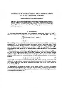
where p denotes the fluid pressure. The condition for (2.3) to hold is that Re = Ωa 2 ρ/µ # 1. The boundary conditions are that u = 0 on the solid boundary, and u is asymptotic to the basic shear flow at large distances from the rigid body. A schematic diagram of the problems is shown in figure 1. Case 1 in figure 1(a) is the shear flow Ωzex past a fixed sphere at the origin. Case 2 in figure 1(b) is the shear Ωzex + U ex past the sphere, where the centre of the sphere is out of the zero-velocity plane of the background shear. The exact velocity field is constructed by employing Stokes doublets associated with the base vectors ex and ey and potential quadrupole in Chwang & Wu (1975). More details about fundamental singularities can be found in their paper. The velocity field u for a fixed sphere in the linear shear is ! " ∂2 1 5a 3 3xzx a 3 ey × x a5 + − ∇ u = Ω zex − 6 r5 2 r3 6 ∂x∂z r % $ & # a3 ∂ 1 (ex x)x 3a ex + + ∇ , (2.4) + U ex − 4 r r3 4 ∂x r

Blocking effects of a sphere in shear flows (a)

(b)

z Primary shear flow (Ωz, 0, 0)

123 z

Primary shear flow (Ωz + U, 0, 0)

y

y x

x

Figure 1. Flow past a fixed sphere x 2 + y 2 + z2 = a 2 . Without loss of generality, assume Ω ! 0 and U ! 0.

' where x = (x, y, z), r = |x| = x 2 + y 2 + z2 , ex , ey and ey are the unit vectors along the x, y and z directions, respectively. The force acting on the fixed sphere is F = 6πµ U ex and the torque at the origin is T = − 4πµ Ω a 3 ez , as shown by Chwang & Wu (1975). Let x & = x/a, u& = u/(aΩ) and U & = U/(aΩ), non-dimensionalizing the equations (dropping the primes), the non-dimensional velocity field is u = zex −

5 xzx ey × x 1 ∂2 1 + − ∇ 2 r5 2r 3 6 ∂x∂z r $ " ! % (ex x)x 3 ex 1 ∂ 1 + + U ex − + ∇ . (2.5) 4 r r3 4 ∂x r

From now on, we use the non-dimensional variables unless stated otherwise. 3. Shear past a sphere whose centre is in the centreplane In this section, we first derive closed formulae for the fluid particle trajectories in the case of an unbounded linear shear past a fixed unit sphere, whose centre lies in the zero-velocity plane of the background shear flow. Then, we investigate the blocking phenomenon based on the trajectory equations. We report results on the flow structure on the y = 0 symmetry plane, followed by results out of this symmetry plane and compare these results with the two-dimensional flow around an infinitely long cylinder. Additionally, we will analytically calculate the stagnation points, the three-dimensional separatrix, and the measurement of blocking regions, and analyse the structure of the flow near the sphere. For this case, the centre of the sphere is in the zero-velocity plane of the background, and the velocity field is a simplified form of (2.5) u = zex −

5 xz x ey × x 1 ∂2 1 + − ∇ . 2 r5 2r 3 6 ∂x∂z r

(3.1)

3.1. Exact quadrature formulae for the fluid particle trajectories Here, streamlines are constructed as the intersection of two stream surfaces for a three-dimensional flow. Of course, it is not always possible to find explicit formulae of streamlines for an arbitrary flow field, and we show how particle trajectories may be computed in closed form for the complex flow studied in this paper.

124


On the basis of the special geometry of this problem, we change the coordinates from rectangular coordinates to spherical coordinates (r, φ, θ ). Using the explicit fluid flow, we may immediately write the particle trajectory equations in spherical coordinates as  3 − 5r 2 + 2r 5 dr    = cos θ sin(2φ) ,   dt 4r 4    2 5 dθ 1 + r − 2r (3.2) = sin θ cot φ ,  dt 2r 5     cos(2φ)(r 5 − 1) + r 5 − r 2  dφ  = cos θ , 5 dt 2r ' where r = x 2 + y 2 + z2 (1 " r < ∞), φ = arccos(z/r) (0 " φ " π) and θ = arctan(y/x) (−π " θ < π). Since ordinary differential equation (ODE) system (3.2) is an autonomous system, we eliminate time t and use the radius r as a new independent variable giving a system for dφ/dr and dθ /dr: (1 + r 2 − 2r 5 ) tan θ dθ = , dr (3r − 5r 3 + 2r 6 ) sin2 φ dφ −r 2 + r 5 + (r 5 − 1) cos(2φ) = . dr r(3 − 5r 2 + 2r 5 ) cos φ sin φ

(3.3) (3.4)

Next, changing the variable y = r sin θ sin φ and taking the derivative of y with respect to r, yields dθ dφ dy = sin θ sin φ + r cos θ sin φ + r sin θ cos φ dr. dr dr

(3.5)

Substituting dθ /dr and dφ/dr into the above equation and replacing sin θ sin φ with y/r, we get dy −5(1 + r) sin θ sin φ −5(1 + r)y = = . dr (r − 1)(3 + 6r + 4r 2 + 2r 3 ) r(r − 1)(3 + 6r + 4r 2 + 2r 3 )

(3.6)

Similarly, take a derivative of z = r cos φ with respect to r and substitute dφ/dr into the resulting formula, dz dφ (1 + r)(5 cos2 φ − 1) = cos φ − r sin φ = . dr dr (3 + 3r − 2r 2 − 2r 3 − 2r 4 ) cos φ

(3.7)

Replacing cos φ with z/r, the above equation becomes dz (r + 1)(r 2 − 5z2 ) = . dr r(r − 1)(3 + 6r + 4r 2 + 2r 3 )z

(3.8)

The obtained ODEs dy/dr and dz/dr decouple. Using separation of variables, ODE (3.6) can be solved analytically. The analytic solution is y 3 = C1

r5 . (r − 1)2 (3 + 6r + 4r 2 + 2r 3 )

(3.9)


125

The ODE in (3.8) is not exact, and hence not immediately separable; nonetheless, an integrating factor may be found. We rewrite this as (1 + r)(r 2 − 5z2 ) dr − z dz = 0. (r − 1)r(3 + 6r + 4r 2 + 2r 3 )

(3.10)

Notice that multiplying this equation by the integrating factor (3 − 5r 2 + 2r 5 )2/3 /r 10/3 yields an exact equation which is solved in closed integral form: , 1/r (1 + s)(1 − s)1/3 (3 − 5r 2 + 2r 5 )2/3 2 ds − z = C2 . (3.11) (2 + 4s + 6s 2 + 3s 3 )1/3 2 r 10/3

Here'C1 and C2 are constants determined by the initial values y0 , z0 and r0 = x02 + y02 + z02 . Equations (3.9) and (3.11) describe the fluid particle trajectories. If r0 (= 1, (3.11) can be rewritten as , 1/r0 (1 + s)(1 − s) 2 r 10/3 ds z2 = 2 5 2/3 (3 − 5r + 2r ) (2 − 5s 3 + 3s 5 )1/3 1/r ! "10/3 ! "2/3 r 3 − 5r02 + 2r05 + z02 . (3.12) r0 3 − 5r 2 + 2r 5

This equation expresses the height z of the fluid particle trajectory in terms of r. These trajectory equations provide rigorous tools for studying the blocking phenomenon.

3.2. Blocking phenomenon Here we analyse the blocking phenomenon which occurs in this flow. This blocking behaviour is a strong modification of the particle trajectories from situations without and with a fixed solid sphere present in the flow: In the absence of a solid sphere, particles released in the shear flow (say, starting above the z = 0 plane) will be swept from large negative x values, to large positive x values as time progresses. However, when the fixed, solid sphere is introduced into the flow, a large measure of particle trajectories lose this streaming property. For example, blocked particles starting with large negative x values do not pass the sphere as time progresses, but rather limit back to large negative x values as time progresses. The regions where this behaviour occurs in three-dimensional space are defined to be the ‘blocked regions’ of the flow; see figure 2, which depicts this blocked region when the flow is restricted to the two-dimensional symmetry plane. We note that this type of behaviour has been observed for the case of an infinitely long cylinder immersed in a linear shear flow by Chwang & Wu (1975); however, they conjectured that this behaviour would not persist in situations involving a sphere (instead of a cylinder). Here, we show that in fact for the case of the sphere, the blocked region persists and, moreover, we analytically compute the geometry of this region, and show that it has infinite crosssectional areas. With the exact, closed-form expressions for the particle trajectories given in (3.9) and (3.12), we may proceed directly to compute the geometry of the blocked regions. 3.2.1. Blocking phenomenon in the y = 0 symmetry plane In the y = 0 plane, the velocity field is " ! 5x 2 z2 − 4x 2 1 , u(x, 0, z) = z 1 − 3 − 5 − 2r 2r 2r 7

(3.13)

126


Figure 2. Streamlines in the y = 0 plane with the linear shear flow zex past a fixed sphere. The four points mark the stagnation points on the unit sphere in this symmetry plane. Note that the separatrix height limits to approximately 0.88207 and is rigorously less than unity.

v(x, 0, z) = 0, (3.14) " ! 2 2 2 1 5z x − 4z w(x, 0, z) = x , (3.15) − 5− 3 2r 2r 2r 7 ' √ and r = x 2 + y 2 + z2 = x 2 + z2 . Notice that one velocity component v vanishes. Particles initially on this plane never leave this plane, i.e. y = 0 for the particle trajectory. Fluid particles in this plane are thus described by the closed integral formula (3.12) with r02 = x02 + z02 and r 2 = x 2 + z2 . The streamlines in the y = 0 symmetry plane shown in figure 2 explicitly depict the blocked region. The fully three-dimensional structure of the blocking region will be described below. The four √ dots on √ the sphere in figure 2 are stagnation points, (x, y, z) = (±2/ 5, 0, ±1/ 5) in rectangular coordinates. Two other stagnation points on the sphere are located at (0, ±1, 0), which are out of this symmetry plane. Stagnation points are special among the fixed points that comprise a no-slip boundary. We define a point on such boundaries to be stagnation points if, for any neighbourhood of one such point, there exists a subset of material fluid points of the neighbourhood that never leave the neighbourhood in backward (for a repelling stagnation point) or forward (for an attracting stagnation point) infinite time. From figure 2, it is clear that there are blocked regions. For example, the flow is separated by the stagnation line in the second quadrant. Below that stagnation line the flow is trapped on the left side of the sphere. It is worth comparing this case with that of the analogous two-dimensional flow. For the two-dimensional flow in the case of an infinitely long cylinder immersed in a linear shear flow with the cylinder axis perpendicular to the lines of constant shear, the stream function is ! "2 " ! 1 1 1 1 1 2 1 − 2 − log r, (3.16) + φ(x, z) = z 1 − 2 2 r 4 r 2 see Chwang & Wu (1975) and Jeffrey & Sherwood (1980) for more details. Here r 2 = x 2 + z2 , and √ the radius of the cylinder is unity. The stagnation points on the cylinder are (± 3/2, ±1/2). Notice that the separatrix is totally explicit in this case.


127

z

x

Figure 3. Separation surfaces generated by separatrix lines in the flow.

Moreover, as x → ± ∞, the height |z| of separatrix goes to ∞. This peculiar behaviour is in some sense similar to the well-known Stokes paradox in a two-dimensional uniform flow past a cylinder. Our results below show that the limiting height of the separatrix is finite in the case involving a fixed, rigid sphere, in sharp contrast with the two-dimensional case. 3.2.2. Blocking phenomenon off the y = 0 plane By continuity, it is expected that the blocking phenomenon extends outside the y = 0 symmetry plane. Our analytic results not only show the existence of this threedimensional blocking region but also establish that the height of the blocking region is bounded by a constant less than the sphere radius, and dependent upon the distance off the symmetry plane. (We will compute explicitly the three-dimensional geometry of the blocked region in §§ 3.4 and 3.5.) Recall (3.9) and (3.12) with the initial value (x0 , y0 , z0 ): .1/3 r 5/3 (r0 − 1)2/3 3 + 6r0 + 4r02 + 2r03 y = y0 5/3 (3.17) .1/3 , r0 (r − 1)2/3 3 + 6r + 4r 2 + 2r 3 ! "2/3 , 1/r0 10/3 (1 + s)(1 − s)1/3 3 − 5r02 + 2r05 2 r 10/3 2 2r z = ds + z0 10/3 , (3 − 5r 2 + 2r 5 )2/3 1/r (2 + 4s + 6s 2 + 3s 3 )1/3 3 − 5r 2 + 2r 5 r0 (3.18) ' where r0 = x02 + y02 + z02 . Particle trajectories are determined by simultaneously solving (intersecting these surfaces) these equations to obtain a curve relating (x, y, z). Figure 3 shows the separation surfaces in the flow. As shown in this figure, there is a region off the x–z plane between the separation surfaces, where the flow is blocked. The vertical plane in this figure shows the cross-section of the blocking region. The area of this cross-section in the limit of x → ±∞ will be discussed in §3.5. Figures 4(a) and 4(b) show the stagnation lines close to the sphere and how they connect to the fixed points in the fluid. In this case, the fixed points are the y-axis outside of the sphere. This curve of fixed points is a subset of the original z = 0 plane of fixed points present in the absence of the rigid sphere. From figure 4(b), it is easy to see that they are hyperbolic fixed points. 3.3. Stagnation points on the sphere Since all points on a solid boundary are fixed points of the flow, special care is needed to define stagnation points which reside on a solid boundary. This degeneracy on

128

R. Camassa, R. M. McLaughlin and L. Zhao (a)

(b) z y

x

Figure 4. (a) Streamlines on separation surface close to the sphere. (b) A zoomed-in view of the cube near the y-axis.

solid boundaries may be split by computing those points on the boundary for which the linearization of the velocity vector field vanishes. These will define the stagnation points on the rigid boundary. Streamlines in the fluid which end at any stagnation point (whether in the fluid or on the boundary) are referred to as stagnation lines. Stagnation lines ending on the boundary are not necessarily perpendicular to the no-slip, rigid boundary. For a 2D flow, the angle between the stagnation line and the rigid surface can be computed, as seen in Pozrikidis (1997). To find the stagnation points on the sphere, we linearize and rescale the velocity equation near the surface of the sphere. When the velocity field in spherical coordinates is linearized with respect to the radius r at 1, the expansions are dr = O((r − 1)2 ), dt dθ = −4 cot φ sin θ(r − 1) + O((r − 1)2 ), dt dφ 3 + 5 cos(2φ) = cos θ(r − 1) + O((r − 1)2 ). dt 2

(3.19) (3.20) (3.21)

After rescaling the time τ = t(r − 1) and neglecting the higher order, we reduce the ODE system to  dr   = 0,   dτ   dθ (3.22) = −4 cot φ sin θ,  dτ    dφ 3 + 5 cos(2φ)  = cos θ.  dτ 2

The steady state of the above ODE system provides the stagnation points, yielding the following conditions: cot φ sin θ = 0,

2 cos θ(5 cos2 φ − 1) = 0.

(3.23)

Since 1 " r " ∞, 0 " φ " π, 0 " θ < 2π, six stagnation points on the sphere are   π 3π   θ = 0, π, ! θ = , , " ! " 2 2 (3.24) r = 1, and 1 1  φ = arccos √ , arccos − √ ,  φ = π. 5 5 2


129

z

y x

Figure 5. ‘Footprint’ of stagnation surfaces on the sphere.

Rewritten in rectangular coordinates, these points are located at " ! 1 2 (0, ±1, 0) and ± √ , 0, ± √ 5 5

(3.25)

(the last points in the y = 0 symmetry plane are plotted in figure 2). The rescaled velocity field provides an imprint of the particle trajectory pattern just off the sphere surface which mathematically reduces to heteroclinic connections between the stagnation points. These connections can be found from the ODE system (3.22), 8 cot φ tan θ dθ =− , dφ 3 + 5 cos(2φ)

(3.26)

and the solution is sin2 θ = C

5 cos2 φ − 1 4 cos2 φ − sin2 φ = C , sin2 φ sin2 φ

(3.27)

where C is a constant depending on the initial value of r, θ and φ. When r = 1, using the stagnation points as initial conditions, we get the equation of the trajectories on the sphere in rectangular coordinates: ' √ (x, y, z) = (±2 cos φ, ± 1 − 5 cos2 φ, ± cos φ), (arccos(1/ 5) < φ < π/2). (3.28)

Or, r = 1 and cos θ = ± 2 cot φ in the spherical coordinates. These trajectories connect the stagnation points in the rescaled flow field and demonstrate the topological structure on the sphere (see figure 5). From these trajectories, in the rescaled coordinates, we classify these stagnation points on the sphere as four nodal points (in the symmetry plane) and two hyperbolic points (on the y-axis). We emphasize that the rescaled flows are a projection onto the sphere, and all of these fixed points in the rescaled system correspond to higher-order (quadratic) hyperbolic points in the original system. We further remark that the entire y-axis exterior to the sphere is a line of fixed points. For finite values along the y-axis, this line is hyperbolic (in the

130


x –z plane) with orientation depending upon the distance from the sphere. Infinitely far from the sphere along the y-axis, these fixed points lose their hyperbolic structure, with the flow becoming a simple shear flow (the background flow). In this limit, the orientation angle tends to zero. In the opposite limit approaching the sphere, this line of hyperbolic points tends to the higher-order hyperbolic fixed point on the sphere, with orientation angle depicted by the geodesic curves in figure 5, with a tangent value 4/3. 3.4. Stagnation lines The precise mathematical definition of the blocked region requires some care to set up. Clearly, the unblocking and blocking regions are divided by the separation surfaces created by stagnation lines in the interior of the fluid as depicted in figures 2 and 3. These regions may be succinctly defined as follows. We define the set of unblocked trajectories to be the set of initial points whose particle trajectories intersect the x = 0 plane off of the y-axis in finite or infinite time. This set of points is topologically open. The complement of this set (thus closed), we define to be the blocking region. Notice that the boundary of this set defines the separation surface. This connected surface contains the separating surface in the fluid, the y-axis, and the sphere surface. To calculate this separation surface, we first identify the stagnation lines using the explicit formulae for the trajectory equations given in (3.9) and (3.12), then study their properties on and off the y = 0 symmetry plane. Through this analysis, we will prove that the height |z| of stagnation lines is finite as x → ±∞ and y fixed.

3.4.1. Stagnation lines in the y = 0 symmetry plane Since one velocity component vanishes in this plane, streamlines are only governed by (3.12)   z2 = !

1

"2/3 3 5 − + 1 2r 5 2r 3

,   

1/r

!

(1 + s)(1 − s)1/3

1 + 2s +

3s 2

3 + s3 2

"1/3

  ds + C , 

(3.29)

where C is determined by the initial value (x0 , 0, z0 ). As we know from the previous √ subsection, √ four stagnation points on the sphere in this symmetry plane are (±2/ 5, 0, ±1/ 5). We use these points as the initial value and get the equation of the stagnation line in this plane , 1 (1 + s)(1 − s)1/3 1 2 (3.30) z = ! ! "1/3 ds. "2/3 3 5 3 3 1/r 2 1 + 2s + 3s + s − 3 +1 2r 5 2r 2 A few remarks regarding this stagnation line may be made. First, the height, z, of the stagnation line is bounded. This is easily seen by replacing the denominator in the integrand by unity and evaluating the integral. This gives a constant slightly bigger than the unit sphere radius. Second, this bound may be improved substantially through dividing the integral into subintervals and further integrand estimates (Zhao 2010). In fact, this ultimately establishes very tight upper and lower bounds for the limiting height value of the stagnation line in the limit x → ∞. This upper bound is less than unity, with value 0.8831, and the lower bound is 0.8811. Numerically, we find |zmax | ≈ 0.88207 as

r → ∞.

(3.31)


131

3.4.2. Stagnation lines off the y = 0 symmetry plane We next calculate the stagnation surface out of the symmetry plane. As shown above, the set of fixed points which are detached from the sphere is the y-axis. Thus, any stagnation line not in the symmetry plane must contain a unique point on the y-axis (as shown in figures 3 and 4, which demonstrate this fact). We use these fixed points as the initial condition r0 = y0 > 1, z0 = 0, and substitute them into the parametric equations for the fluid particle trajectory to obtain stagnation lines lying outside of the symmetry plane .1/3 r 5/3 (y0 − 1)2/3 3 + 6y0 + 4y02 + 2y03 , (3.32) y = y0 5/3 y0 (r − 1)2/3 (3 + 6r + 4r 2 + 2r 3 )1/3 , 1/y0 (1 + s)(1 − s)1/3 2r 10/3 2 z = (3.33) .2/3 .1/3 ds. 1/r 3 − 5r 2 + 2r 5 2 + 4s + 6s 2 + 3s 3

This provides the equations for the stagnation lines out of the symmetry plane. Notice that the stagnation line in the symmetry plane terminates on the sphere at a point which is not on the y-axis. Thus, next we investigate how the points on the separation surface close to the symmetry plane topologically connect stagnation lines intersecting the y-axis with the stagnation line in the symmetry plane. (Because of the symmetry of the flow, we only consider the case of y0 close to +1.) Using the y-coordinate of the stagnation lines crossing the y-axis given in (3.32), with an initial condition (0, 1+δ, 0) (δ # 1), which is a point close to (0, 1, 0), we have "1/3 ! "−1/3 "−2/3 ! ! 2 1 2 3 3 δ (15 + 20δ + 10δ 2 + 2δ 3 ) 1− 1+ + 2 + 3 . (3.34) y= 2(1 + δ)2 r r r 2r As r → ∞, this limits to

!

15 2

"1/3

δ 2/3

!

4δ 2 2 2 1+ + δ + δ3 3 3 15 2/3 (1 + δ)

"1/3

,

(3.35)

and, as δ → 0, the leading-order approximation is (15/2)1/3 δ 2/3 . This shows that the out of the symmetry plane stagnation line crossing the fixed point (0, y0 , 0), which is sufficiently close to the stagnation point (0, 1, 0) on the sphere, asymptotically approaches the stagnation line in the y = 0 plane as r → ∞ (we note that the z-value given in (3.33) trivially converges in this limit to the limiting height computed above). This property guarantees that the blocking region at x = ∞ is completely characterized by the separation lines which intersect the y-axis. This will be very useful in measuring the cross-sectional area of the blocking region. 3.5. Cross-sectional area of the blocking region as x → ∞ We next study the geometry of this blocking region far from the body. We do this by examining its cross-sectional structure (as in figures 3 and 6). Unfortunately, at finite distances from the body, this cross-sectional region of intersecting the plane x = L with the stagnation surface is not readily provided by the equations in (3.32) and (3.33) as they are parametrized by the spherical radius. Fortunately, we can overcome this difficulty by working with L → ∞ since r ∼ x in this limit. In this limit, the formulae in (3.32) and (3.33) provide (y, z) coordinates for the curves bounding the blocking region (shown for large, but finite L, in figure 6). While from this figure it is clear that the height z = z(y) will decay to zero as y → ∞, the limiting procedure yields a parametric representation (with parameter y0 ) for this

132

R. Camassa, R. M. McLaughlin and L. Zhao z

y

Figure 6. Cross-section of the bounded blocking region at infinity (viewed from upstream).

curve. To obtain the decay rate of z(y) as y → ∞ (which is critical to determine if the cross-sectional area is infinite) requires further analysis, as we next show. From the equations of the stagnation lines (3.32) and (3.33), we get ! "2/3 ! "1/3 1 2 3 3 1+ + 2+ 3 , (3.36) y ∼ y0 1 − y0 y0 y0 2y0 , 1/y0 (1 + s)(1 − s)1/3 2 (3.37) z2 ∼ ! "1/3 ds = (z∞ ) , 3 0 3 1 + 2s + 3s 2 + s 2

as r → ∞ by taking x → ∞, where z∞ > 0. Here y0 , a point on the y-axis, parametrizes the trajectory determined by the equations for y and z above. This parametric representation for the curve z = z(y) may be viewed as an image of the y-axis under the flow after infinite time, which we may use to derive an explicit expression for the cross-sectional area. To wit, the Jacobian matrix for this mapping is "1/3 ! 3 5 5 (1 + y0 ) dy = 1+ 5 − 3 + ! "1/3 ! "2/3 . (3.38) dy0 2y0 2y0 1 4 6 3 4 2+ 2y0 1 − + 2+ 3 y0 y0 y0 y0 The area of the blocked flow is noted as I , , ∞ , ∞ I dy = z(y) dy = z∞ (y0 ) dy0 4 dy0 0 1 "1/3 , ∞ ! 3 5 = z∞ 1 + 5 − 3 dy0 2y0 2y0 1 , ∞ 5 (1 + y0 ) + z∞ ! "1/3 ! "2/3 dy0 1 4 6 3 1 4 2+ 2y0 1 − + 2+ 3 y0 y0 y0 y0 = part 1 + part 2.

(3.39)

For the integral part 2, the leading order of the integrand 5 (1 + y0 ) ! "1/3 ! "2/3 1 4 6 3 4 2+ 2y0 1 − + 2+ 3 y0 y0 y0 y0

(3.40)

is 5 (3.41) 2 (2)2/3 y03 as y0 → ∞. Notice that the integrand in (3.37) is bounded. Consequently, an upper √ bound for the decay of z∞ is 1/y0 as y0 → ∞. Thus, the integral part 2 is bounded.


133

We next show that the integral part 1 diverges: "1/3 , ∞ ! 5 3 Part 1 = z∞ 1 − 3 + 5 dy0 . 2y0 2y0 1

Substitute z∞ (y0 ) in (3.37) into the integrand  Part 1 =

,

1

∞ , 1/y0

As y0 → ∞,

  

0

!

(1 + s)(1 − s)1/3

3 1 + 2s + 3s 2 + s 3 2 !

"1/3

5 3 1− 3 + 5 2y0 2y0

1/2

  ds  

"1/3

!

→ 1.

1−

5 3 + 2y03 2y05

(3.42)

"1/3

dy0 . (3.43)

(3.44)

Using the following result to estimate the integral in the kernel (which follows directly through straightforward Taylor expansion), , η (1 + s)(1 − s)1/3 η3 + O(η4 ). (3.45) ! "1/3 ds = η − 3 3 0 3 2 1 + 2s + 3s + s 2

This establishes the following asymptotic expansion: , 1/y0 (1 + s)(1 − s)1/3 1 as y0 → ∞. (3.46) ! "1/3 ds ∼ y0 3 3 0 2 1 + 2s + 3s + s 2 √ Therefore, the integrand 8of √ part 1 is asymptotic to 1/y0 as y0 → ∞. With such a ∞ decay rate, the integral 1 1/y0 dy0 = ∞ is divergent. Since the integrand is sign definite, this result shows that part 1 is divergent. Consequently, the total area of the cross-section of the blocking region is infinite when the plane x = x0 → ∞. In the y–z plane (i.e. x = 0), the blocking region is the y-axis, i.e. the area of the cross-section is zero. This is in sharp contrast with the calculation just presented above, where it was shown that at x = ∞, the cross-section of the blocking region is infinite. Since the explicit, closed-form formula for the area at an arbitrary distance from the sphere is not available, we study its behaviour by analysing the integrand involved here under different asymptotic limits. We will see a continuous connection between zero cross-sectional blocking area at x = 0 and diverging cross-sectional blocking area as x → ∞. The separation surface is generated by the stagnation lines crossing the fixed points (0, y0 , 0) on the y-axis, where |y0 | > 1. If we take the cross-section of the blocking region at x0 , then y 2 + z2 = r 2 − x02 . On the basis of the trajectory equations (3.32) and (3.33), we have ! "2/3 , 1/y0 - 2 . 3 1 5 1 (s + 1)(1 − s)1/3 2 − + 1 − x r = "1/3 ds ! 0 2 r5 2 r3 3 3 1/r 2 s + 3s + 2s + 1 2 ! "2/3 3 1 5 1 − + 1 . (3.47) + y02 2 y05 2 y03

134


From the above equation, we find the mapping from r to y0 with x0 fixed. With such a mapping, the boundary of the cross-section of the blocking area can be written as parametric functions & y = y (r (y0 ) , y0 ) (3.48) z = z (r (y0 ) , y0 ) at x = x0 fixed. The leading-order asymptotic solution to (3.47) is 9 r ∼ y02 + x02 as y0 → ∞ and x0 fixed.

(3.49)

If a = (0, z) and n is the outer normal direction of the cross-section, dy z(y0 ) dy :0 . a · n = :: : dy : : : dy0 :

(3.50)

By the divergence theorem or Gauss’ theorem, the cross-section of the blocking area I is an explicit integral: " , , , , ∞! dy I = dA = div a dA = a · n ds = (3.51) z(y0 ) dy0 . 4 dy0 1 Ω Ω ∂Ω From the asymptotic result (3.49) and several applications of the implicit function theorem to obtain derivative asymptotics (we relegate these technical √ details to Appendix A), we find that for finite x0 , the integrand decays as x0 /( 2y03/2 ), when y0 → ∞, which yields a finite cross-sectional blocking area. To study the behaviour for the blocking area as x0 increases, we take the crosssection at x0 = y0) , where ) > 0 is a constant. ' (i) When 0 < ) < 1, from (3.47), we find r ∼ y02 + y02) as y0 → ∞. Substitute this into the√ integrand for the blocking area, the integrand for the blocking area is asymptotic to (1/ 2)(1/y03/2−) ). When 0 < ) < 1/2, the integral is convergent. Otherwise, 1/2 < ) < 1, the integral is divergent. ' (ii) If the cross-section is taken at x0 = y0) () ! 1), then r ∼ y02) + y02 as y0 → ∞. In √ this case, the integrand of (3.51) for the blocking area decays as 3/(2 y0 ) as y0 → ∞. This illustrates an unreported property about the solution of the Stokes flow but physically not observed. Since, at large distance, the characteristic length used in the Reynolds number need to be redefined, the inertia terms ignored in the Navier–Stokes equation are not negligible. 4. Shear past a sphere whose centre off the zero-velocity plane of the primary shear flow When the centre of the unit sphere x 2 + y 2 + z2 = 1 is out of the zero-velocity plane of the background shear flow illustrated in figure 1, the non-dimensional primary linear shear flow can be written as U = zex + U ex , in which the uniform flow rate U is related to the shear rate and the distance between the centre of the sphere and the zero-velocity plane of the shear flow. Without loss the generality, we can assume U > 0. While we will not be able to obtain a closed-form explicit solution in these off-centre cases as before, we will explicitly compute the fixed-point structure in closed form.


135

The exact velocity field for the flow is given in (2.5). We rewrite the velocity field as an ODE system in spherical coordinates:  dr U r(1 + 2r) + (3 + 6r + 4r 2 + 2r 3 ) cos φ  2 = (r − 1) cos θ sin φ,    4  dt 2r    2 3 2 5 U r(1 + 3r − 4r ) + 2(1 + r − 2r ) cos φ dθ (4.1) = sin θ,  dt 4r 5 sin φ      dφ U r(1 + 3r 2 − 4r 3 ) cos φ + 4(1 − r 5 ) cos2 φ + 2(r 2 − 1)   =− cos θ, 5 dt 4r where 1 " r < ∞, 0 " φ " π and 0 " θ < 2π. From the above ODE system (4.1), we apply the same approach as we have used in the previous section to attain the ODEs dy/dr and dz/dr. Skipping the details of changing variables and taking derivatives, we get dy/dr and dz/dr with the radius r as a new independent variable: . (1 + r) 3r 2 U + 10z y dy ; . 0, the corresponding point (x, y, z) from (4.15) is a hyperbolic fixed point. If F (r, U ) < 0, and the point (x, y, z) satisfying (4.15) is an elliptical fixed point. Otherwise, when F (r, U ) = 0, the point of (4.15) is a higher-order fixed point with all three eigenvalues being zero. When U = 8/3, the finite curve shrinks into a point and collapses with the four stagnation points on the sphere, and all the fixed points in the interior of the fluid are now on the infinite-length curve. After U ! 8/3, fixed points in the interior of the fluid are always on such a curve. The quantified streamline plots shown in figures 10 and 11 document the qualitative bifurcation sketches in figure 9. In figure 10, we show fixed point curves in the flow and the flow structure in the x–z symmetry plane with given U . Notice that the fixed points are plotted in the y–z plane, since the fixed points in the fluid are only in the y–z plane. In figures 10 and 11, the first column shows the different values of U studied, and the second column shows plots for curves of fixed points from (4.15) (the grey area indicates the sphere). The third column shows streamline patterns obtained numerically in the x–z symmetry √ plane, i.e. the lateral view. The first value U = (16/9) 2 < U * is picked corresponding to stage 1 in the bifurcation sketches of figure 9. In this case, as shown in the second column, fixed points are on two infinite-length curves, each of whose end point is a stagnation point on the sphere. With this special value, the curves of fixed points in the y–z plane have infinite slope at the stagnation point. With the second value U = 2.64837 ≈ U * , a cubic parabolic (cusp) fixed point appears. In the third row U * < U = 2.64912 < U ** , the fixed points in the fluid are on two new curves. Both end points of the finite length curve are stagnation points on the sphere, and the curve with infinite length is asymptotic to a line in the zero-velocity plane of the background shear flow. With the fourth value U = 2.65059 ≈ U ** in figure 11, the fixed points in the interior of the fluid are still on two curves. The stagnation lines in the streamline plot in the symmetry plane connect the hyperbolic fixed point in the fluid with the stagnation points on the sphere, and separate closed orbits around the elliptical fixed point from the open trajectories. For U ** , we do not have an explicit formula for this value and use the numerical approximation 2.65059. For the fifth value U ** < U = 2.65287 < 8/3, the elliptical fixed points moves up as U increases, and there are fluid particles which pass the sphere from the left to the right between the elliptical fixed point and the hyperbolic fixed point. The last case U = 8/3 shows that fixed points are on one curve in the interior of the fluid. These numerical results clearly show the existence of the blocking regions when the sphere is out of the zero-velocity plane of the primary shear flow. The streamline plots in the y = 0 plane show the interesting bifurcation appearing in the fluid particle trajectories. When U * < U < 8/3, streamlines show a 3D eddy near the elliptical fixed points below the sphere. Figure 12 shows the circulation near the elliptical fixed points below

Blocking effects of a sphere in shear flows (a) Front view

143

(b) Lateral view

Figure 12. (a, b) Circulation near elliptical and hyperbolic fixed points below the sphere. Grey surface marks the surface of the sphere.

(a) Front view

(b) Lateral view

z z

y

x

y

x

(c) 3D view

z

y

x

Figure 13. (a–c) Circulation near elliptical and hyperbolic fixed points below the sphere.

the sphere when U = 2.6514. Figure 12(a) is the front view of fluid particle trajectories and figure 12(b) is their lateral view. From figure 12(b), it is clear that these are closed trajectories circulating around the elliptical fixed points on the finite-length fixed point curve in and out of the symmetry plane. From the front view in Figures 12(a) and 13(a), we see that trajectories are further deformed when they are close to the surface of the sphere and approaching the hyperbolic fixed point on the finite-length fixed point curve.

144

R. Camassa, R. M. McLaughlin and L. Zhao (a)

(b)

z y

z x

y

x

Figure 14. (a, b) Closed and open streamlines below the sphere exhibiting the streamline pattern bifurcation.

Figures 13 and 14 show streamlines in the y < 0 half-space below the sphere. In figure 13, the streamlines are only closed orbits near the fixed points on the finitelength curve (here we take U = 2.6514). Figure 13(a) is the front view, figure 13(b) is the lateral view, and figure 13(c) is the 3D view. These orbits are selected so that they are around the elliptical points, but near the sphere they are close to the hyperbolic fixed points on the finite-length fixed point curve. Figure 14 shows both closed and open streamlines near the fixed points.

5. A sphere embedded in rotating flows To further explore similar phenomena, we next consider the flow with a sphere embedded in rotating flows. The centre of the sphere is set at the origin of the coordinate system. The background flow is a rigid-body rotation in the x–y plane with the rotation axis parallel to the z-axis and translated a fixed distance L from the origin. In this case, the x–y plane is the symmetry plane of the flow. The planar linear shear case with the sphere centre at some distance off the zero-velocity plane may be viewed as an extreme case of this rotating background flow in that at large distances L, the curvature of rigid-body rotation streamlines over regions of sphere radius scales becomes negligible. However, there are important differences with respect to the planar case in the interpretation of blocking regions for the case of a rotating background flow past a sphere, as in this case the definition of blocking itself becomes fundamentally different. We will study the case when the sphere is fixed in the rotating flow first and then allow the sphere to additionally self-rotate. For a sphere self-rotating in the rotating background flow, we report results about the flow in cases when the sphere may freely self-rotate and the cases when the sphere self-rotates at a prescribed angular velocity. The rotation axis of the self-rotation of the sphere is the z-axis. For a sphere embedded in such rotating flows, we will next find the explicit fluid particle trajectories from the exact velocity field and document the analytical formula for stagnation points on the sphere and the fixed points in the interior of the fluid. 5.1. A fixed sphere in the rotating flow When the unit sphere is embedded in purely rotating flows, the background flow can be decomposed into a uniform flow plus two linear shear flows in rectangular coordinates, whose origin is the centre of the sphere. Assuming that the non-dimensional angular velocity of the rotation is (0, 0, 1) and the distance between the rotation axis and theorigin is L ! 0, the background flow is yex − (x + L)ey . When the sphere is fixed,


145

with no-slip boundary condition on the surface of the sphere, the velocity of the flow can be obtained from (2.4), @  ?  y 3Lxy 3Lxy  u(x, y, z) = y − .3/2 + .3/2 − .5/2 ,     4 x 2 + y 2 + z2 4 x 2 + y 2 + z2 x 2 + y 2 + z2    x   v(x, y, z) = −L − x + .3/2   2 2 2 + y + z x ? @  3 L 1 + 3y 2 3y 2   ' + +−, . .  3/2 5/2  2 2 2 2 2 2 2 2 2 4  x +y +z x +y +z x +y +z     3Lyz 3Lyz   + . w(x, y, z) = − .5/2 .3/2  2 2 2 2 2 2 4 x +y +z 4 x +y +z (5.1) Similar to the planar shear past a sphere, we calculate the fluid particle trajectories for this velocity field by obtaining explicit formulae in terms of r, E √ F √ √ 2 r 2 log(2 r + 2(1 + 2r)) − 8C 27 2 1 r (5 + 4r) √ , (5.2) + x= 8L(1 − r) 16L(1 − r) r(1 + 2r) z2 =

C2 r 3 , (r − 1)2 (1 + 2r)

y 2 = r 2 − x 2 − z2 ,

(5.3) (5.4)

where C1 and C2 are constants determined by the initial position of the fluid particle. To present the structure of the flow, we plot fluid particle trajectories with different values of L in the x–y symmetry plane. When L = 0, trajectories are shown in figure 15(a). In this case, it is clear from the velocity field (5.1) that there is no motion in the z-direction and all velocity components vanish along the z-axis (x = y = 0). When 0 < L < 2, trajectories are illustrated in figure 15(b) with a specified value L = 1. There are two stagnation points on the sphere and they are in the x–z plane, shown in figure 17(b), where we show the stagnation points on the sphere. When L = 2, trajectories are shown in figure 15(c). There is one stagnation point on the sphere at (−1, 0, 0). When L > 2, trajectories are plotted in figure 15(d ) with L = 3. There are two stagnation points on the sphere. Figure 16 is the 3D view of figure 15(d ). As figures 15 and 16 implied, the stagnation points on the sphere depend √ on the distance L. For√a unit sphere, there are two stagnation points (−L/2, 0, 4 − L2 /2) and (−L/2, 0, 4 − L2 /2) on the sphere if 0 " L < 2. When L = 2, there is only one stagnation point (−1, 0, 0) on the √ sphere. When L > 2, there are √ still two stagnation points on the sphere at (−2/L, ( L2 − 4/L), 0) and (−2/L, −( L2 − 4/L), 0), but they are in the x–y symmetry plane instead of the x–z plane for L < 2. Furthermore, we get the formula for fixed points in the interior of the fluid, which are only in the x–z plane. The implicit formula for fixed points in the fluid is 3L L + 4x . .3/2 = L + x − √ 2 4 x + z2 4 x 2 + z2 -

(5.5)

146


(a) L = 0

(b) L = 1

(c) L = 2

(d) L = 3

Figure 15. Trajectories in the x–y symmetry plane for the case of a rotating background flow.

In parametric formulae, they are L 1 + s + 4s 2 , 4 1 + s + s2 ' √ 16s 2 (1 + s + s 2 )2 + L2 (1 + s + 4s 2 )2 , z = ± s2 − x2 = ± 4(1 + s + s 2 )

x=−

(5.6) (5.7)

where |s| ! 1. When L " 2, fixed √ points in the interior of√the fluid connect to the two stagnation points (−L/2, 0, 4 − L2 /2) and (−L/2, 0, 4 − L2 /2) on the sphere as shown in figures 17(a) and 17(b). Solid dots on the sphere are stagnation points in figure 17. Since fixed points in the fluid are only in the x–z plane, plots in figure 17 are restricted to the x–z plane. The solid curve in figure 17(a) shows the location of fixed points when L = 0. Figure 17(b) shows the location of fixed points when L = 1. For the degenerate case L = 2 shown in figure 17(c), the curve connects to the unique stagnation point (−1, 0, 0) on the sphere. Otherwise, for L > 2, as in figure 17(d ) (L = 3), fixed points are on a curve that is still in the x–z plane but is away from the sphere. All the curves are asymptotic to the rotation axis of the background flow as |z| → ∞. Notice the analogy of these curves of fixed points with those identified off


147

z y x

Figure 16. 3D view of trajectories in the x–y symmetry plane when L > 2.

(a) L = 0

z

(b) L = 1

2

2

0

0

–2

–2

–2

0

2

(c) L = 2

z

–2

0

2

–2

0

2

(d ) L = 3

2

2

0

0

–2

–2

–2

0

x

2

x

Figure 17. (a–d ) Fixed points in the fluid in the x–z plane when a fixed sphere is embedded in a rotating background flow. L is the distance from the rotation axis of the background flow to the centre of the unit sphere.

148


the x–z plane by the analysis of the linear planar shear case in § 4. The force acting on the fixed sphere is F = − 6πµLey and the torque at the origin is T = − 8πµey in dimensionless formulae. 5.2. A self-rotating sphere in the rotating flow If the sphere self-rotates in the rotating background flow, imposing the no-slip boundary condition on the rotating sphere requires the velocity on the surface of the sphere to be u& = − γ yex + γ xey . For the special torque-free case involving a sphere freely self-rotating at the origin, the angular velocity of the self-rotation is set to γ = −1, as the calculation shows. The exact velocity field is 3Lxy (γ + 1)y 3Lxy − − 2 , (5.8) 2 2 3/2 2 2 2 5/2 +y +z ) 4(x + y + z ) (x + y 2 + z2 )3/2 4x(γ + 1) + L(1 + 3y 2 ) 3L + v(x, y, z) = −L − x + ' 4(x 2 + y 2 + z2 )3/2 4 x 2 + y 2 + z2 3Ly 2 − , (5.9) 2 4(x + y 2 + z2 )5/2 3Lyz 3Lyz − . (5.10) w(x, y, z) = 2 2 2 3/2 2 4(x + y + z ) 4(x + y 2 + z2 )5/2 u(x, y, z) = y +

4(x 2

And the equation of fluid particles is the following parametric system: G ?I @ H ' 1 3r r3 ' − √ 64γ 3(1 + 2r)arctanh x= 1 + 2r 24 (1 + 2r) 2L (r − 1)2 r 3 (1 + 2r) J K ' ' √ √ + 3(2 r(5 + 14r + 8r 2 ) + 27 2(1 + 2r) log(2 r + 2(1 + 2r))) − C1 , (5.11) z2 =

r3 , C2 (r − 1)2 (1 + 2r)

y 2 = r 2 − x 2 − z2 ,

(5.12)

(5.13)

where constants C1 and C2 depend on initial values. Fixed points in the interior of the fluid are

 L 3 2  (4r − 3r − 1), 4(γ + 1 − r 3 )  z2 = r 2 − x 2 . x=

(5.14)

The slope of the fixed-point curve as depicted in figure 18 is 2γ /3L at (0, 0, 1), the top of the sphere. For the degenerate cases L = 0 and γ > − 1, the velocity vanishes not only on the curve prescribed by (5.14) in the x–z plane but also on the shell x 2 + y 2 + z2 = (1 + γ )2/3 . For the special case γ = 0 (with the sphere fixed), the location of stagnation points on the sphere depends on L as shown in figure 17. Figure 18 shows the fixed points in the x–z plane for different values of L when the sphere is freely self-rotating in the rotating background flow. Figure 19 shows the fluid particle trajectories of the freely self-rotating case in the x–y symmetry plane for different values of L. Figure 20 shows trajectories of fluid particles out of the x–y symmetry plane, when L = 4 and the sphere is freely rotating. When the orientation of the sphere self-rotation is opposite and equal to that of the background flow, figure 21 shows fixed points in the x–z plane and figure 22 shows

Blocking effects of a sphere in shear flows (a) L = 0

z

(b) L = 2

2

2

0

0

–2

–2

–3

–2

–1

0

1

2

3

(c) L = 3.330407

z

–3

2

0

0

–2

–2

–2

–2

–1

0

1

2

3

(d ) L = 4

2

–3

149

–1

0

x

1

2

3

–3

–2

–1

0

1

2

x

Figure 18. (a–d ) Same as figure 17 but for the case of the sphere freely self-rotating in a rotating background flow.

the trajectories of fluid particles in the x–y symmetry plane with different values of L. Figure 23 shows the structure of the fluid particle trajectories out of the symmetry plane when L = 3. A comparison between these figures shows that the location of the hyperbolic fixed point may be positioned either on the left or on the right side of the sphere, depending upon the parameters. 6. Conclusion and discussion We have presented an analysis of the fluid particle trajectories for linear shear and rotating flows past a rigid sphere or spheroid in viscosity-dominated regimes. For the symmetric case of a fixed sphere with its centre located on the zero-velocity plane of the linear shear, closed-form expressions provide a complete characterization of the blocking regions. When the sphere centre moves at some distance off this plane, local bifurcations occur in the distance parameter which are analysed analytically, with

150

R. Camassa, R. M. McLaughlin and L. Zhao (a) L = 0

(b) L = 2

(c) L = 3.330407

(d) L = 4

Figure 19. (a–d ) Trajectories in the x–y symmetry plane with a freely-rotating sphere.

z y

x

Figure 20. Trajectories out of the x–y symmetry plane when the sphere is freely rotating and L = 4.

numerical computations showing the persistence and deformations of the blocking regions associated with global bifurcations. For the case involving a background flow past a sphere in rigid-body rotation around a vertical axis, exact expressions for the fluid particle trajectories were presented in all cases. These include the case of a fixed-centre sphere off the axis of the background flow rotation with or without arbitrarily imposed vertical spinning, which may be of importance for studies of

Blocking effects of a sphere in shear flows (a) L = 0

(b) L = 0.02

2

2

0

0

–2

–2

z

–3

–2

–1

0

1

2

3

(c) L = 1

z

–3

–2

–1

0

1

2

3

–2

–1

0

1

2

3

(d ) L = 3

2

2

0

0

–2

–2

–3

151

–2

–1

0

x

1

2

3

–3

x

Figure 21. (a–d ) Same as figures 17 and 18 but with a unit sphere self-rotating in an opposite direction with respect to the background flow.

mixing processes. This case is reminiscent of that occurring in the linear background shear flow for large distances off the sphere centre from the zero-velocity plane. Lastly, we have analysed how some of these phenomena are altered when spheres are deformed into prolate spheroids. This introduces an additional orientation to the fluid–body interaction set-up which makes its parametric study much richer. We have concentrated on a subset of this parameter space whence the major spheroid axis lies on the x–z plane. A new behaviour of the fluid flow has emerged in this study, which does not have a counterpart in the spherically symmetric case, namely fluid particle trajectories may be attracted or repelled out of the x–z plane, in positive and negative suction-like patterns. The associated blocking phenomena documented in Appendix A for spheroids are further expected to improve the understanding of the unusual fluid particle trajectories reported by Camassa, Leiterman & McLaughlin (2008) and more

152

R. Camassa, R. M. McLaughlin and L. Zhao (a) L = 0

(b) L = 0.02

(c) L = 1

(d) L = 3

Figure 22. (a–d ) Trajectories in the x–y symmetry plane when the sphere is self-rotating in an opposite direction with respect to the background flow.

z y

x

Figure 23. Trajectories out of the x–y symmetry plane when the sphere is self-rotating in an opposite direction with respect to the background flow.

generally to understand the flow induced by the motion of cilia in biological systems, such as those examined by Bouzarth et al. (2007). Of particular interest is the behaviour and analysis of the cross-sectional scales of the blocked region. For the case of a fixed sphere centred on the zero-velocity plane, asymptotic estimates were provided which document that this blocking crosssection diverges at large distances from the sphere. We believe that this is the generic behaviour for Stokes’ parallel shear flows in exterior domains past rigid bodies. Naturally, this behaviour is somewhat unphysical and should be viewed as yet another form of the Stokes paradox, although in the case of shear emerges in a milder form than e.g. the infinite volume dragged by a uniformly moving sphere. Future studies will investigate the inertial corrections for this unphysical behaviour using matched asymptotics along the lines of the Oseen theory. Such an analysis was


153

performed by Bretherton (1962) for the special two-dimensional case involving a disk, who showed that logarithmic divergence of the stagnation streamlines bounding the blocked region is suppressed by the inertial terms, making the streamlines settle upon finite height asymptote at infinity. A similar analysis appears to be more involved for the case of a sphere and to our knowledge has never been done. Additional worthy investigations along these lines include assessing behaviours arising from a temporally fluctuating shear flow and/or sphere location as well those associated with more complex rheologies. Finally, the presence of realistic boundary conditions on the exterior fluid domain should be addressed to compare with experiments such as those reported by Poe & Acrivos (1975). R.C. was partially supported by NSF DMS-0509423 and NSF DMS-0620687. R.M.M. was partially supported by NSF DMS-0308687, RTG NSF DMS-0502266 and NSF NIRT 0507151. L.Z. was partially supported by NSF DMS-0509423 and NSF NIRT 0507151. We thank D. Adalsteinsson for his visualization software DataTank and NSF DMS-SCREMS 04224 for computer support.

Appendix A. Cross-sectional blocking area asymptotics In this Appendix, we provide the details about the decay rate of the integrand used to compute the cross-sectional area of the blocking region. When the integrand decays fast enough, the integral is convergent, which implies that the cross-sectional area of the blocked region is finite. Otherwise, the integral is divergent and the cross-sectional area is infinite. The closed integral form trajectory equations (3.32) and (3.33) of the fluid particles are ! "2 ! " 1/3 3 1 1 1 1 +3 2 +2 +1   1− y 2 y03 y0 y0   0 (A 1) y = y0  ! "2 ! "  ,   1 3 1 1 1 1− +3 2 +2 +1 r 2 r3 r r , 1/y0 1 (s + 1)(1 − s)1/3 (A 2) z2 = ! "1/3 ds. "2/3 ! 3 3 5 3 1/r 2 s + 3s + 2s + 1 1+ 5 − 3 2r 2r 2 Substituting y and z into the original ODE system used to derive the trajectory equations, we have " ! 1 +1 y 5 dy r . = dr (1 − r) 3 + 6r + 4r 2 + 2r 3 ! "2 ! "1/3 " ! 1 3 1 1 1 1 +3 2 +2 +1  +1 5y0  1− y 2 y03 y0 y0 r   0 (A 3) = ! "2 ! "  , 2 3 (1 − r)(3 + 6r + 4r + 2r )   1 3 1 1 1 1− +3 2 +2 +1 r 2 r3 r r

154

R. Camassa, R. M. McLaughlin and L. Zhao " 5 2 (1 + r) 2 z − 1 dz r r = 2 3 4 dr 3 + 3r − 2r − 2r − 2r z  !



, 1/y0 5  1 (s + 1)(1 − s)1/3   (1 + r)r 2 ! "2/3 "1/3 ds − 1 ! r  3 1 3 3 5 1 1/r s + 3s 2 + 2s + 1 − +1 5 3 2r 2r 2 =  1/2.       , 1/y0   1/3 (s + 1)(1 − s) 1 (3 + 3r − 2r 2 − 2r 3 − 2r 4 ) ! ds ! "2/3 "1/3   3 1 3 3 5 1 1/r   2   − + 1 s + 3s + 2s + 1   5 3 2r 2r 2 (A 4) All these four equations are in terms of r and y0 . If x = x0 , from x 2 = r 2 − y 2 − z2 , we derive the following constraint: ! "2/3 - 2 . 5 3 1− 3 + 5 r − x02 2r 2r ! "2/3 , 1/y0 (s + 1)(1 − s)1/3 5 3 2 1 − = ds + y + . ! "1/3 0 2y03 2y05 3 3 1/r 2 s + 3s + 2s + 1 2

(A 5)

Taking implicit differentiation, we have dr = dy0

L 2y05 − y02 − 1 ! "2/3 ! "1/3 5 5 3 3 1− 3 + 5 y04 1 − 3 + 5 2r 2r 2y0 2y0 "! "  !  3 1 1   1+ 5 − 1+  1− r 2  10y0 (1 + r) 2y0 r  ! " + 2 + 2r 3 )  5  3 5 r(r − 1)(3 + 6r + 4r   r2 1 − 3 + 5 1− 3 + 2r 2r 2r     , 1/y0  (s + 1)(1 − s)1/3 5(1 − r 2 ) + 2r − ! "5/3 ! "1/3 ds .  5 3 3 3 1/r   s + 3s 2 + 2s + 1 r6 1 − 3 + 5  2r 2r 2

2/3 5 2y03   3  2r 5 (A 6)

Also, from the trajectory equation, we get ∂y (r, y0 ) =− ∂y0

-

. y05 − 1 ! "1/3 ! "2/3 , 5 5 3 3 1− 3 + 5 y05 1 − 3 + 5 2r 2r 2y0 2y0

(A 7)

∂z(r, y0 ) =− ∂y0

Blocking effects of a sphere in shear flows ! "! " 1 1 1− 1+ y0 y0 1/2 

155

 , 1/y0 (s + 1)(1 − s)1/3    ! "1/3 ds    1/r 3 3 s + 3s 2 + 2s + 1 2 ! "−1/3 5 3 1− 3 + 5 2r 2r ×! "1/3 . 3 5 1+ 5 − 3 2y0 2y0 2y02

(A 8)

Now all the components involved in the integral in § 3.5 are in terms of r and y0 . If a = (0, z), then dy z a · n = A! " dr ! " , 2 2 dz dy + dr dr

ds =

A!

dz dr

"2

dz dy0

"2

+

!

dy dr

+

!

dy dy0

"2

dr,

(A 9)

or z a · n = A!

dz dy0

dy dy0

"2

+

!

dy dy0

"2 , ds =

A!

"2

dy0 .

(A 10)

Note the area of the 2D cross-section as I . By the divergence theorem, the area of the 2D cross-section of the blocking region is , , , ∞ , dy dr I = dA = div a dA = a · n ds = z dy0 4 dr dy0 1 Ω Ω ∂Ω " , ∞ ! ∂y ∂r ∂y dy0 . = z + (A 11) ∂r ∂y0 ∂y0 1 We will analyse the integrand involved in the cross-sectional area of the blocking region, " ! ∂y ∂y ∂r , (A 12) + z ∂r ∂y0 ∂y0 to study the property of the cross-sectional area of the blocking region. Substituting (A 1)–(A 8) into the above integrand, we eventually write it as a function of r and y0 ,  1/2 " ! , 1/y0  (1 + s)(1 − s)1/3 1 ∂y ∂y ∂r   =! + ds z "2/3  ! "1/3  ∂r ∂y0 ∂y0   5 3 3 3 1/r 1− 3 + 5 s + 3s 2 + 2s + 1 2r 2r 2

156

R. Camassa, R. M. McLaughlin and L. Zhao " " "! ! ! 1 1 1 3 L 1 + 2 − 2y0 5 1+ 1− 5 r y0 y0 × ! "2/3 − "2/3 !  5 3 5 3   y0 (1 − r)(3 + 6r + 4r 2 + 2r 3 ) 1 − 3 + 5  1− 3 + 5 2r 2r 2y0 2y0  ! "2/3 3 5 1 1022/3 y02 1 + 5 − 3  1− 2 2y0 2y0  r " + ! 2r − 5 3 r(1 − r)(3 + 6r + 4r 2 + 2r 3 )  2 r 1− 3 + 5 2r 2r     , 1/y0   2 1/3 (s + 1)(1 − s) 5(1 − r )  − ! (A 13) "5/3 ! "1/3 ds  .  5 3 3 3 1/r  2 6  s + 3s + 2s + 1 r 1− 3 + 5  2r 2r 2     

If x0'is a fixed finite number, from the constraint (A 5), we get the asymptotic solution r ∼ y02 + x02 . Substitute this solution into the above equation. The integrand ! " ∂y ∂r ∂y x0 z + (A 14) ∼ √ 3/2 as y0 → ∞. ∂r ∂y0 ∂y0 2y0 At a finite distance |x0 | from the sphere, the cross-sectional area of the blocking region depends on x0 and is finite. If the cross-section is taken at infinite x0 = ∞, then ?! "2 ! "@1/3 1 3 3 2 1− 1+ 3 + 2 + , (A 15) y ∼ y0 y0 y0 2y0 y0 , 1/y0 (s + 1)(1 − s)1/3 z2 ∼ (A 16) ! "1/3 ds. 3 3 0 2 s + 3s + 2s + 1 2 The cross-sectional area I is computed as , , , , ∞ I dy = dA = div a dA = a · n ds = z dy0 . 4 dy 0 1 Ω Ω ∂Ω

The integrand decays as  z

1/2 

, 1/y0  (s + 1)(1 − s)1/3 dy   ∼ ds ! "1/3  dy0  0  3 3 s + 3s 2 + 2s + 1 2 ! "7/2 5 1 1 as y0 → ∞. ∼ √ + 3 y0 y0

2/3

2   

. - 5 y0 − 1

!

y05 3 − 5y02 + 2y05 y05

(A 17)

"2/3     

(A 18)

With such a decay rate, the integral is divergent. Far enough from the sphere, the cross-sectional area is infinite. To understand the growth of the area, we assume 'x0 = y0) () > 0), then from the constraint (A 5) we get the asymptotic solution r ∼ y02 + y02) . Substituting this

Blocking effects of a sphere in shear flows Primary shear flow (Ωz, 0, 0)

157

z

y x

Figure 24. A linear shear flow passes a fixed prolate spheroid. The major axis is perpendicular to the direction of the shear flow (an upright spheroid).

solution into the integrand (A 13) and computing the asymptotic as y0 → ∞, we have the following. (i) When 0 < ) < 1, as y0 → ∞, the leading order of the integrand (A 13) is " ! y −(3/2)+) ∂y ∂r ∂y ∼ − 0√ as y0 → ∞. z + (A 19) ∂r ∂y0 ∂y0 2 As y0 → ∞, the integrand decays like y0−(3/2)+) . Consequently, when 0 < ) < 1/2, the integral is convergent. When ) ! 1/2, the integral is divergent. (ii) When ) ! 1, as y0 → ∞, the leading order of the integrand (A 13) is ! " ∂y ∂r 3 ∂y z ∼ − √ + as y0 → ∞. (A 20) ∂r ∂y0 ∂y0 2 y0 In this case, the cross-sectional area of the blocking region is infinite. Appendix B. Shear flow past a spheroid In this Appendix, we focus on the flow structure and blocking phenomena for a prolate spheroid embedded in a linear shear flow. With respect to the spherical case, the spheroid orientation relative to the background shear enriches the phenomena, some of which will be examined here. The literature on this set-up has concentrated mostly on forces and torques (Blaser 2002), while some experimental investigations of three-dimensional separation structures for flows past spheroids can be found in the high Reynolds regime (Wang et al. 1990). First, we report results about the shear flow Ωzex when the spheroid sits with its centre on the zero-velocity plane and its major axis upright (as shown in figure 24), x2 + y2 z2 + =1, (B 1) b2 a2 where a > b are the major and minor semi-axes, respectively, and the half focal length c and the eccentricity e are defined as c = (a 2 − b2 )1/2 = e a. From Chwang & Wu (1975), the exact velocity field in this case is , c (c2 − ξ 2 )(αU SS (x − ξ ; ez , ex ) + γ U R (x − ξ ; ey )) dξ u(x) = Ωzex − −β

,

c

−c

−c

(c2 − ξ 2 )2 ∂z U D (x − ξ ; ex ) dξ,

(B 2)

158

R. Camassa, R. M. McLaughlin and L. Zhao z

x

Figure 25. Streamlines in the y = 0 symmetry plane for a linear shear past a fixed upright spheroid. The four points mark the stagnation points on the spheroid.

where U SS , U R and U D are the fundamental singularities of stresslet, rotlet and doublelet, located at ξ , 3((x − ξ ) · ez )((x − ξ ) · ex ) (x − ξ ), R5 (x − ξ ) × ey UR (x − ξ , ey ) = , R3 ex 3(x − ξ ) · ex UD (x − ξ , ex ) = − 3 + (x − ξ ), R R5

USS (x − ξ ; ez , ex ) =

with R =

(B 3) (B 4) (B 5)

' x 2 + y 2 + (z − ξ )2 , and ξ = ξ ez . Here, α, β and γ are known constants,

α=β

−2e + (1 − e2 )Le 4e2 2 = γ e , 1 − e2 2e(2e2 − 3) + 3(1 − e2 )Le

γ =

Ω , −2e + (1 + e2 )Le

(B 6)

and Le = log ((1 + e)/(1 − e)). Numerical results show the existence of blocked regions in the flow, as shown in figure 25, where the streamlines are plotted in the y = 0 symmetry plane. B.1. Stagnation points on the spheroid From the velocity field (B 2), we find the stagnation points on the spheroid. As before for the spherical case, we first rewrite the velocity field in prolate spherical coordinates  x = a e sinh(µ) sin(ν) cos(φ),   y = a e sinh(µ) sin(ν) sin(φ),   z = a e cosh(µ) cos(ν),

(B 7)

where arccosh(1/e) " µ " ∞, 0 " ν " π and −π " φ < π (more details about the explicit velocity field are provided by Zhao 2010). Next, we rescale the time τ = (µ − arccosh(1/e)) t and expand the velocity field near the no-slip boundary of the spheroid where µ = arccosh(1/e), ignoring higher-order terms of order (µ − arccosh(1/e))2 . The linearized ODE system for the trajectory of fluid particle


159

near the surface of the spheroid reduces to          

dµ = 0, dτ k(e) dν cos(φ) = 4 ωe3 , dτ d(e) e2 + e2 cos(2ν) − 2

where

     2 4 2  dφ [2e(3 − e ) + (e + 2e − 3)L ] cot(ν) sin(φ)  e 3  = 4 ωe ,  dτ d(e) 1 − e2

(B 8)

d(e) ≡ 12e2 − 8e4 + 4e(e4 + e2 − 3)Le − 3(e4 − 1)L2e

(B 9)

k(e) ≡ 2e(6 − e2 ) + (e4 + 3e2 − 6)Le + e2 cos(2ν)((1 + e2 )Le − 2e).

(B 10)

dν = 0 and dτ

(B 11)

and

The conditions for stagnation points on the boundary, dµ = 0, dτ

dφ = 0, dτ

define six stagnation points on the upright prolate spheroid in the prolate spherical coordinates ! " E π πF 3π π , a arccosh(1/e), , , (B 12) a arccosh(1/e), , 2 2 2 2 ? ? ! "1/2 @@ 6e − (3 − e2 )Le a arccosh(1/e), 0, arccos ± (B 13) 2e3 − e2 (1 + e2 )Le

and

a

? ! "1/2 @@ 6e − (3 − e2 )Le . arccosh(1/e), π, arccos ± 2e3 − e2 (1 + e2 )Le

?

(B 14)

In the original rectangular coordinates, the latter stagnation points lie in the y = 0 symmetry plane ? ! "1/2 "1/2 @ ! √ 6e − (3 − e2 )Le 6e − (3 − e2 )Le 2 , 0, ± , (B 15) a ± 1−e 1− 3 2e − e2 (1 + e2 )Le 2e3 − e2 (1 + e2 )Le √ while the other two are on the y-axis at (0, ±a 1 − e2 , 0). The location of the stagnation points in the y = 0 symmetry plane migrates towards the spheroid ‘tips’ with increasing eccentricity e at fixed a. The four points merge into two at the tips in the ‘needle’ limit of eccentricity e → 1, while for the opposite limit of a sphere (e → 0) we retrieve the previous result (3.25). Just like for the spherical case, the zero-velocity plane of the background shear flow collapses to just the y-axis for the upright spheroid whose centre is on this plane. B.2. Characterization of stagnation streamlines on the surface of the spheroid As for the case of the sphere, the rescaled velocity field provides an imprint of the particle trajectory pattern just off the spheroid surface which mathematically reduces to heteroclinic connections between the stagnation points (see figure 26).

160 (a)

R. Camassa, R. M. McLaughlin and L. Zhao (b)

z

(c)

z

y y

z

x

x

Figure 26. (a–c) ‘Footprint’ of stagnation surfaces on the spheroid surface from different viewpoints.

From the rescaled velocity field ODE (B 8), we get dν (1 − e2 )k(e) cot(φ) tan(ν) = 2 , dφ (e cos(2ν) + e2 − 2)[2e(3 − e2 ) + (e4 + 2e2 − 3)Le ]

(B 16)

sin(φ) sin(ν) = C (k(e))p(e) ,

(B 17)

whose solution is

where the constant C is determined by the initial conditions, and the constant p(e) is p(e) ≡

2e + (e2 − 1)Le . (1 − e2 )((1 + e2 )Le − 2e)

(B 18)

Substituting the stagnation points yields the trajectories

x 2 = (1 − e2 )(a 2 − z2 ) − y 2 = a 2 (1 − e2 ) sin2 (ν) − y 2 , √ √ y = a 1 − e2 sin(ν) sin(φ) = a 1 − e2 C(k(e))p(e) , z = a cos(ν),

(B 19) (B 20) (B 21)

in the first octant (x, y, z positive), which can be extended by the symmetry of the flow to the whole space. B.3. Linear shear flow past a tilted spheroid When the major axis of the spheroid is tilted with an angle κ, defined as the angle between the positive z-axis and the major axis of the spheroid in the x–z plane (see figures 27a and 28a), the y = 0 plane is still a symmetry plane of the flow but the up-down symmetry of the fluid–body set-up is broken. The tilted prolate spheroid is (x sin(κ) + z cos(κ))2 (x cos(κ) − z sin(κ))2 + y 2 + = 1 (a > b > 0). (B 22) b2 a2 (The previous case is recovered for κ = 0.) The solution of Stokes equations for this tilted case can be efficiently obtained in the body frame from the general theory of Chwang & Wu (1975) and Jeffery (1922). In this frame, the spheroid’s major axis is on the x-axis, and the background flow can be decomposed into two shear flows xey and yex and an elongational flow xex − yey . For each of these shear flows, the velocity field is given by changing coordinates

Blocking effects of a sphere in shear flows (a) Configuration

(b) Streamlines

161

z

z y x

Figure 27. (a–b) Blocked streamlines near the separation surface in the y < 0 half-space when the spheroid is tilted towards the shear with κ = −π/4. Particles initially distributed on a curve within the blocked region move downwards while being attracted towards the body as indicated by the perspective arrow on the right.

of (B 2) for the first one, and , c u(x) = yex + (c2 − ξ 2 )(α3 U SS (x − ξ ; ex , ey ) + γ3 U R (x − ξ ; ez )) dξ −c , c (c2 − ξ 2 )2 ∂y U D (x − ξ ; ex ) dξ, + β3

(B 23)

−c

for the second, respectively. Here γ3 =

1 − e2 , −2e + (1 + e2 )Le

β3 =

(1 − e2 )(Le − 2e) γ3 4e(2e2 − 3) + 6(1 − e2 )Le

and α3 =

4e2 β3 . 1 − e2 (B 24)

For the elongational flow Ωxex − Ωyey , the velocity field is (Jeffery 1922)

u = x{Ω + β & (W − V ) − 2(α + 2β)A} 2xP 2 − 2 [{W − 2(a 2 + λ)A + 2(b2 + λ)B}y 2 (a + λ)3/2 (b2 + λ)3 − {V − 2(b2 + λ)C + 2(a 2 + λ)A}z2 ], (B 25) & & v = y{−Ω + α U − β W − 2(α + 2β)B} 2yP 2 − 2 [{U − 2(b2 + λ)B + 2(b2 + λ)C}z2 /(b2 + λ)2 (a + λ)1/2 (b2 + λ)2 − {W − 2(a 2 + λ)A + 2(b2 + λ)B}x 2 /(a 2 + λ)2 ], (B 26) & & w = z{β V − α U − 2(α + 2β)C} 2zP 2 − 2 [{V − 2(b2 + λ)C + 2(a 2 + λ)A}x 2 /(a 2 + λ)2 (a + λ)1/2 (b2 + λ)2 − {U − 2(b2 + λ)B + 2(b2 + λ)C}y 2 /(b2 + λ)2 ], (B 27)

162

R. Camassa, R. M. McLaughlin and L. Zhao (a) Configuration

z

x

(b) Streamlines z

y

Figure 28. (a–b) Similar to figure 27, blocked streamlines near the separation surface in the y < 0 half-space, when the spheroid is tilted along the shear with κ = π/4.

where 1 2 (x + y 2 + z2 − a 2 − b2 2' + (x 2 + y 2 + z2 − a 2 − b2 )2 + 4{a 2 (y 2 + z2 − b2 ) + b2 x 2 }), "−1 ! x2 y 2 + z2 2 + 2 , P = (a 2 + λ2 )2 (b + λ)2 λ=

and α=

,

∞

(a 2

λ

α& =

,

λ

1

∞

√

λ)3/2 (b2

+

1 dλ, a 2 + λ(b2 + λ)3

α && = β − b2 α & ,

The constants A–W are A=

Ω , 6β0&&

+ λ)

dλ,

B=Ω

β=

,

∞

λ

β& =

,

λ

1 √ dλ, 2 a + λ(b2 + λ)2

∞

1 (a 2

+

λ)3/2 (b2

+ λ)2

dλ,

β && = α − b2 β & . −2β0&& − α0&& , 6β0&& (β0&& + 2α0&& )

C=Ω

−α0&& + β0&& , 6β0&& (β0&& + 2α0&& )

(B 28) (B 29)

(B 30) (B 31) (B 32)

(B 33)

Blocking effects of a sphere in shear flows (a) For an upright spheroid (κ = 0)

163

z

y

z

(b) κ = –π/4

y

z

(c) κ = π/4

y

Figure 29. Cross-section of the blocked region at x = −5 fixed.

U =−

Ωb2 , 2α0&& + β0&&

V =

Ωb2 (β0&& − α0&& ) Ωa 2 − , 3β0&& (β0&& + 2α0&& ) 3β0&&

W =

Ωa 2 Ωb2 (2β0&& + α0&& ) + , 3β0&& 3β0&& (β0&& + 2α0&& ) (B 34)

where α0&& = and

3 − e2 (e2 + 3)Le − 4a 3 e4 (1 − e2 ) 8a 3 e5

(B 35)

−6e + (3 − e2 )Le (B 36) 2a 3 e5 are α && and β && evaluated at λ = 0, respectively. (More details about the velocity field in the original laboratory frame are provided by Zhao 2010.) As for the other cases we have discussed, six stagnation points on the tilted spheroid are obtained by rescaling the velocity field in prolate spherical coordinates and linearizing it near the surface. Two of the stagnation points are located at β0&& =

164


(0, ±b, 0), while the location of the other four are defined by the solutions of the following equation in prolate spheroid coordinates: cos(2κ) cos(2ν) 3(1 − e2 )Le + 2e(2e2 − 3)

{22e3 − 18e + (9 − 14e2 + 5e4 )Le } sin(2κ) sin(2ν) − √ 2 1 − e2 (6e + (e2 − 3)Le )(2e(5e2 − 3) + 3(e2 − 1)2 Le )

+

12e − 8e3 − 6(1 − e2 )Le + (6e + (e2 − 3)Le )e2 cos(2κ) = 0. e2 (3(1 − e2 )Le + 2e(2e2 − 3))((1 + e2 )Le − 2e)

(B 37)

This equation yields two values of the angle ν between 0 and π, corresponding to two stagnation points on the spheroid in the y = 0 symmetry plane. In the original rectangular coordinates, where the spheroid is tilted in the shear flow, these two stagnation points are defined by substituting such solutions ν into √     −sin(κ) cos(ν) − 1 − e2 cos(κ) sin(ν) xs     0 (B 38)  ys  = a  . √ zs cos(κ) cos(ν) − 1 − e2 sin(κ) sin(ν) Using the specular symmetry of the set-up with respect to the origin in the y = 0 plane locates the other two stagnation points. Figures 27 and 28 are plots of numerically evaluated streamlines from the above exact velocity field in the laboratory frame which illustrates the main features of the flow. When the spheroid is tilted in the x–z plane, the portion of the y-axis in the fluid turns into a stagnation streamline, as opposed to a line of fixed points for the upright case, i.e. points on the y-axis move in the y-direction. However, the y-axis keeps its feature of being the intersection of separation surfaces bounding the blocked region of fluid. For a given spheroid, the maximum speed on the y-axis streamline is achieved at a certain finite location on this axis for the tilt corresponding to the angle κ = ± π/4. The speed along the y-axis is zero on the body and at infinity. (i) When the spheroid is tilted towards the background linear shear (κ < 0), on the y-axis, the flow pushes the fluid particles towards to the spheroid. Figure 27(a) shows the configuration of the linear shear and the tilted spheroid with κ = − π/4, and figure 27(b) shows the positive suction of the fluid particles when the particle trajectories are close to the separation surface. (ii) When the spheroid is tilted along the background linear shear (κ > 0), on the y-axis, the flow pushes the fluid particles away from the spheroid. The configuration of the linear shear and the tilted spheroid with κ = π/4 is shown in figure 28(a), and the negative suction of the fluid particles is illustrated with the blocked fluid particle trajectories close to the separation surface in figure 28(b). For the cross-section of the blocked region, when the spheroid is upright or horizontal, i.e. when its major axis is aligned along the z- or x-axis, respectively, the up-down symmetry (reflections with respect to the x–y plane) of the set-up is preserved; in this case, the cross-section is symmetric, as shown in figure 29(a). This is similar to the spherical case in figure 6, but notice that corners develop on the bounding surfaces along the y = 0 plane. The cross-section height is a decreasing function of y. When the spheroid is tilted in the x–z plane, the up-down symmetry of the cross-section is also broken: when the spheroid is tilted against the background


165

stream (κ < 0), both boundaries of the cross-section are concave upward near y = 0; when the spheroid is tilted along the background linear shear (κ > 0), both boundaries of the cross-section are concave downward near y = 0. Figures 29(b) and 29(c) are cross-sections of the blocked region with κ = − π/4 and κ = π/4, respectively. Near the corners, the concavity of the boundaries of the blocked region is determined by the spheroid eccentricity e and the tilt angle κ. From the local analysis near the stagnation points (B 38) in the symmetry plane, the eigenvectors of the matrix of the linearized velocity in√the general body frame, where the spheroid is along the x-axis, are (0, 0, a) and a(0, 1 − e2 sin(ν), cos(ν)). When these two vectors are perpendicular to each other, i.e. the eccentricity e and the tilt angle ±κ satisfy 12e − 8e3 − 6(1 − e2 )Le + (6e + (e2 − 3)Le )e2 cos(2κ) e2 (3(1 − e2 )Le + 2e(2e2 − 3))((1 + e2 )Le − 2e) cos(2κ) − = 0, (B 39) 2 3(1 − e )Le + 2e(2e2 − 3) the concavity of the blocked region changes. REFERENCES Blaser, S. 2002 Forces on the surface of small ellipsoidal particles immersed in a linear flow field. Chem. Engng Sci. 57, 515–526. Bouzarth, E. L., Brooks, A., Camassa, R., Jing, H., Leiterman, T. J., Mclaughlin, R. M., Superfine, R., Toledo, J. & Vicci, L. 2007 Epicyclic orbits in a viscous fluid about a precessing rod: theory and experiments at the micro- and macro-scales. Phys. Rev. E 76 (1), 016313, 1–5. Bretherton, F. P. 1962 Slow viscous motion round a cylinder in a simple shear. J. Fluid Mech. 12, 591–613. Camassa, R., Leiterman, T. J. & McLaughlin, R. M. 2008 Trajectory and flow properties for a rod spinning in a viscous fluid. Part 1. An exact solution. J. Fluid Mech. 612, 153–200. Chwang, A. T. & Wu, T. Y. 1975 Hydromechanics of low-Reynolds-number flow. Part 2. Singularity method for Stokes flows. J. Fluid Mech. 67, 787–815. Cox, R. G., Zia, Y. Z. & Mason, S. G. 1968 Particle motion in sheared suspensions. XXV. Streamline around cylinders and spheres. J. Colloid Interface Sci. 27, 7–18. Feke, D. L. & Schowalter, W. R. 1983 The effect of Brownian diffusion on shear-induced coagulation of colloidal dispersions. J. Fluid Mech. 133, 17–35. Jeffrey, D. J. & Sherwood, J. D. 1980 Streamline patterns and eddies in low-Reynolds-number flow. J. Fluid Mech. 96, 315–334. Jeffery, G. B. 1922 The motion of ellipsoidal particles immersed in a viscous fluid. Proc. R. Soc. Lond. A 102, 161–179. Kim, S. & Karrila, S. J. 2005 Microhydrodynamics: Principles and Selected Applications. Dover. Kossack, C. A. & Acrivos, A. 1974 Steady simple shear flow past a circular cylinder at moderate Reynolds numbers: a numerical solution. J. Fluid Mech. 66, 353–376. Leal, L. G. 2007 Advanced Transport Phenomena: Fluid Mechanics and Convective Transport Processes. Cambridge University Press. Ma, T. & Wang, S. 2001 A generalized Poincar´e–Hopf index formula and its applications to 2-D incompressible flows. Nonlinear Anal. Real World Appl. 1, 467–482. Mikulencak, D. R. & Morris, J. F. 2004 Stationary shear flow around fixed and free bodies at finite Reynolds number. J. Fluid Mech. 520, 215–242. Poe, G. G. & Acrivos, A. 1975 Closed streamline flows past rotating single cylinders and spheres: inertia effects. J. Fluid Mech. 72, 605–623. Pozrikidis, C. 1997 Introduction to Theoretical and Computational Fluid Dynamics. Oxford University Press.

166


Robertson, C. R. & Acrivos, A. 1970 Low Reynolds number shear flow past a rotating circular cylinder. Part 1. Momentum transfer. J. Fluid Mech. 40, 685–704. Saffman, P. G. 1965 Lift on a small sphere in a slow shear flow. J. Fluid Mech. 22, 385–400. Spielman, L. A. 1977 Particle capture from low-speed laminar flows. Annu. Rev. Fluid Mech. 9, 297–319. Wang, K. C., Zhou, H. C., Hu, C. H. & Harrington, S. 1990 Three-dimensional separated flow structure over prolate spheroids. Proc. R. Soc. Lond. A 421, 73–91. Zhao, L. 2010 Fluid–structure interaction in viscous dominated flows. PhD thesis, University of North Carolina at Chapel Hill.

Lagrangian blocking in highly viscous shear flows

Lagrangian blocking in highly viscous shear flows

Suggest Documents

Galerkin Least-Squares Solutions for Purely Viscous Flows of Shear ...

Critical Layers in Shear Flows

Viscous flows in two dimensions - CiteSeerX

Noncircular converging flows in viscous gravity

PULSATILE VISCOUS FLOWS IN ELLIPTICAL VESSELS AND

LAGRANGIAN FLOWS FOR VECTOR FIELDS

Lagrangian statistics in unforced barotropic flows

Lagrangian structures in time-periodic vortical flows

Lagrangian PTV in 3D flows - Springer Link

Shear Flows and Shear Viscosity in a Two-Dimensional Yukawa ...

Tracer diffusion in granular shear flows

Shear Stress Effects in Cavitating Flows

Shear dispersion in dense granular flows

Modeling of turbulent shear flows

Shallow waters viscous flows for arbitrary topography

A hyperbolic model for viscous Newtonian flows

FLUID MECHANICS Chapter 8: Viscous flows

Alternating currents and shear waves in viscous electronics

Phase-field simulations of viscous fingering in shear-thinning fluids

Stability of vorticity defects in viscous shear - UBC Math

Inviscid and Viscous Interactions in Subsonic Corner Flows

Some Viscous in Fully Developed Cavity Flows - Caltech Authors

A novel approach to rigid spheroid models in viscous flows

Liquid interfaces in viscous straining flows: Numerical studies of the ...