SPIE's 14th International Symposium on Sensors and Smart Structures Technologies for Civil, Mechanical, and Aerospace Systems, 18 March - 22 March, 2007, paper # 6529-25
Lamb Waves Time-reversal Method using Frequency Tuning Technique for Structural Health Monitoring Buli Xu Mechanical Engineering Department, University of South Carolina Columbia, SC 29208,
[email protected] Victor Giurgiutiu Mechanical Engineering Department, University of South Carolina Columbia, SC 29208,
[email protected]
ABSTRACT Lamb wave time reversal method is a new and tempting baseline-free damage detection technique for structural health monitoring. With this method, certain types of damage can be detected without baseline data. However, the application of this method to thin-wall structures is complicated by the existence of at least two Lamb wave modes at any given frequency, and by the dispersion nature of the Lamb wave modes existing in thin-wall structures. The theory of Lamb wave time reversal has not yet been fully studied. This paper addresses this problem by developing a theoretical model for the analysis of Lamb wave time reversal in thin-wall structures based on the exact solutions of the Rayleigh-Lamb wave equation. The theoretical model first used to predict the existence of single-mode Lamb waves. Then the time reversal behavior of singlemode and two-mode Lamb waves is studied numerically. The advantages of single-mode tuning in the application of time reversal damage detection are highlighted. The validity of the proposed theoretical model is verified through experimental studies. In addition, a similarity metric for judging time invariance of Lamb wave time reversal is presented. It is shown that, under certain condition, the use of PWAS-tuned single-mode Lamb waves can greatly improve the effectiveness of the time-reversal damage detection procedure.
1. INTRODUCTION 1.1.
GUIDED WAVES FOR STRUCTURAL HEALTH MONITORING
Structural health monitoring (SHM) is an emerging research area with multiple applications in the evaluation of the safety and reliability of critical structures. A typical SHM system for in-situ structural interrogation consists of a network of piezoelectric wafer active sensors (PWAS) and a data collection and interpretation unit. The PWAS in the system are small surface-mounted transceivers capable of generating and detecting Lamb waves in thin-wall structures [1]. As guided waves, Lamb waves can travel for long distance with little amplitude loss and permit the inspection of large areas of thin-wall structures from a single location [2]. Some examples of SHM with Lamb wave include crack detection in aluminum plates, delamination detection in composite plates, and corrosion detection in pipes [3][4][5]. 1.2.
ISSUES IN GUIDED WAVE FOR STRUCTURAL HEALTH MONITORING
Application of Lamb waves for SHM is complicated by the existence of at least two modes at any given frequency, and by the dispersion nature of the modes. When a guided wave mode is dispersive, an initial excitation starting in the form of a pulse of energy will spread out in space and easily get overlapped with the reflection from the defects in the structure. This fact worsens the spatial resolution and makes experimental data hard to interpret, especially for long distance testing. Some researchers have tried to compensate this dispersion numerically by taking into account the dispersion characteristics of the guided wave modes. However, their work needs accurate group velocity data for the structure, involves extensive computation, and is not effective for real-time SHM system [6][7]. Furthermore, traditional guided wave SHM techniques developed from nondestructive evaluation (NDE), such
1
as pitch-catch method, pulse-echo method, etc., depend on the availability of a pristine structure baseline to assess the structural health. The detection is performed through the examination of the guided wave amplitude, phase, dispersion, and the time of the flight in comparison with the “pristine” situation. These methods may be sensitive not only to small changes in the material stiffness and thickness, but also to the temperature changes. The baseline measured at one temperature, may not be a valid baseline for the measurement made at another temperature. Moreover, maintenance of the baselines database needs extensive memory space. All these aspects limit the application of guided waves for SHM. These issues encountered and manifested in traditional guided wave SHM methods, may be overcome by a new approach based on the time reversal principle [8]. 1.3.
TIME REVERSAL PRINCIPLE
The concept of time-reversal was initially introduced in physical science community [9]. Within the range of sonic or ultrasonic frequencies where adiabatic processes dominate, the acoustic pressure field is described by a G G G scalar p (r , t ) that, within a heterogeneous propagation medium of density ρ (r ) and compressibility κ (r ) , satisfies the equation G 1 G G (1) Where, Lr = ∇ ⋅ ( G ∇), Lt = −κ (r )∂ tt . ρ (r ) This equation is time-reversal invariant because Lt contains only second-order derivatives with respect to time (selfadjoint in time), and Lr satisfies spatial reciprocity since interchanging the source and the receiver does not alter the resulting fields. G ( Lr + Lt ) p (r , t ) = 0
In a non-dissipative medium, Equation (1) guarantees that for every burst of sound that diverges from a source, there exists a set of waves that would precisely retrace the path of the sound back to the source. This fact remains true even if the propagation medium is inhomogeneous with variations of density and compressibility which reflect, scatter, and refract the acoustic waves. If the source is pointlike, time reversal allows focusing back onto the source whatever the medium complexity [10]. gi(t)
f(t)
Figure 1
gi(-t)
f(-t)
Two operation steps of time-reversal procedure using acoustic time-reversal mirror [11]
The generation of such a converging wave has been achieved by using the so called time-reversal mirrors (TRM). Figure 1 illustrates the two operation steps of the time-reversal mirror [11]. In the first step (left), a source f(t) emits waves that propagate out and are distorted by in homogeneities in the medium. Each transducer in the mirror array detects the wave arriving at its location and feeds the resulting signal gi(t) to a computer; in the second step (right), each transducer plays back the reversed signal gi(-t) in synchrony with the other transducers. In accordance with the time invariance of Equation (1), the original wave is re-created traveling backward, thus retracing its passage back through the medium, untangling its distortions and refocusing on the original source point as f(-t). As we can see, after the time reversal procedure, the source f(t) is reversed and reconstructed as f(-t) and the wave is refocused onto its original source point. These two time reversal properties have been used in many applications based on bulk waves such as underwater acoustics, telecommunications, room acoustics, ultrasound medical imaging, and therapy [10].
2
1.4.
LAMB WAVE TIME REVERSAL
Due to the complexity of the Lamb waves, time reversal of Lamb waves is relatively new and has only been explored by a few researchers. Time reversal method has been tried to transmit a dispersed Lamb wave over a particular distance and obtain a simple waveform with improved SNR and space resolution for NDE applications [12]. Also, time reversal method has been used to focus Lamb wave energy to detect flaws or damages in plates [13][14][15]. More recently, Lamb wave time reversal method was introduced as a baseline-free SHM technique [8][16]. This technique uses the reconstruction property of the time reversal procedure, i.e., an original wave can be reconstructed at its source point if its forward wave recorded at another point is time reversed and emitted back to the source point. However, when damage is presented in the structure between the source and receiver, the forward wave may be mode converted, scattered or reflected by the damage, and the reconstruction procedure may break down. Thus, the reconstructed wave can be compared directly with its original already known source to tell the presence of the damage in the structure without using a baseline. In addition, time reversal procedure recompresses a dispersive wave, improves the spatial resolution of the testing, and makes the experimental data easier to interpret. Park et al. [16] conducted Lamb wave time reversal experiment to detect damage on plate. As shown in Figure 2, damage was simulated by steel block attached between two surface-bonded PWAS, A and B. Without the block attached, the time-reversal reconstructed wave is close in shape to the original wave. But when the block is attached, the reconstructed wave differs from the original wave. Thus, the presence of the damage was detected by comparing the shapes of the reconstructed wave and the original input. PWAS A
Figure 2
Time reversal experiment for attached steel block detection: (a) a steel block (5.0cm H × 4.5cm W × 0.6cm T) attached between PWAS A and B; (b) normalized original input and reconstructed signals at PWAS A [16]
Although Lamb wave time-reversal technique has been attempted experimentally and shows its effectiveness for detecting certain types of damage, the theory of Lamb wave time reversal has not been fully studied. An approximation to Lamb wave time reversal based on Mindlin plate wave theory was presented in ref. [17]. It predicts time reversal of flexural wave, which is a good approximation of A0 mode Lamb wave at low frequency range, but it is incapable of analyzing the other widely used Lamb wave mode, such as S0 mode, or the multi-mode Lamb waves, such as S0+A0 modes. More importantly, it is not accurate because it does not include PWAS model into the theory. This paper will first review previous work on PWAS Lamb wave theory and mode tuning with PWAS transducers on isotropic metallic plates [18]. Next, a theoretical model for the analysis of Lamb wave time reversal using PWAS transducers will be proposed. To validate the theory, time reversal of single mode (S0 mode or A0 mode) and two-mode (S0+A0 mode) Lamb waves will be studied numerically and experimentally. Finally, time invariance of the Lamb wave time reversal will be discussed.
2. THEORY OF PWAS LAMB WAVE TIME REVERSAL 2.1.
LAMB WAVE
Lamb waves, a.k.a. guided plate waves, are a type of ultrasonic waves that remain constrained between two parallel free surfaces, such as the upper and lower surfaces of a plate or shell. Lamb wave theory, which is fully documented in several textbooks [19][20][21], assumes the 3-D wave equations in the form of
3
∂ 2φ ∂x 2 + ∂ 2φ ∂y 2 + ω 2φ c 2p = 0
(2)
∂ 2ψ ∂x 2 + ∂ 2ψ ∂y 2 + ω 2ψ cs2 = 0
where φ and ψ are potential functions, c 2p = (λ + 2 μ ) ρ and cS2 = μ ρ are the pressure (longitudinal) and shear
(transverse) wave speeds, λ and μ are the Lame constants, and ρ is the mass density. The potentials are solved by imposing strain-free boundary condition at the upper and lower faces of the plate. Lamb wave in plate can be modeled in rectangular [22] or cylindrical coordinates [23]. In the first case, Lamb wave is assumed to be straight crested, while in the second case, Lamb wave is assumed to be circular crested. In both cases, by applying the stress-free boundary conditions at the upper and lower surfaces, Rayleigh-Lamb wave equation can be obtained: tan β d tan α d = ⎡⎣ 4ξ 2αβ (ξ 2 − β 2 ) 2 ⎤⎦
±1
(3)
where, d is the half thickness of the plate, c is the phase velocity, and ξ is the wave number, and α 2 = ω 2 c 2p − ξ 2 ,
β 2 = ω 2 cs2 − ξ 2 , ξ 2 = ω 2 c 2 . The plus sign corresponds to symmetric (S) motion and minus to anti-symmetric (A) motion. Equations (3) accepts a number of eigenvalues, ξ 0S , ξ1S , ξ 2S , ... and ξ 0A , ξ1A , ξ 2A , ... , respectively. To each eigenvalue corresponds a Lamb wave mode shape. The symmetric modes are designated S0, S1, S2, …, while the antisymmetric are designated A0, A1, A2, …. Since the coefficients α and β in depend on the angular frequency ω, the eigen values ξiS and ξiA are functions of the excitation frequency. The corresponding wave speeds (phase velocity), given by ci = ω ξi , will also be functions of the excitation frequency. The change of wave speed with frequency produces wave dispersion of a wave packet. At a given frequency thickness product fd, each solution of the Rayleigh-Lamb equation generates a corresponding Lamb wave speed and a corresponding Lamb wave mode. Also, there exists a threshold frequency value determined by the material of the plate and the plate thickness, below which, only S0 and A0 modes exist. At low frequencies, the S0 Lamb wave mode can be approximated by an axial plate wave; and the A0 Lamb wave mode can be approximated by a flexural plate wave.
2.2.
PWAS TRANSDUCER
In recently years, several investigators have explored the generation and detection of structural wave with piezoelectric wafer active sensors (PWAS) transducers. Most of the methods used in conventional guided-wave NDE, such as pitch-catch, pulse echo, and phase arrays, have also been demonstrated experimentally with PWAS [1][2][5]. These successful experiments have positioned PWAS as an enabling technology for the development and implementation of active SHM methods. PWAS operate on the piezoelectric principle: an alternating voltage applied to the PWAS terminals produces an oscillatory expansion and contraction of the piezoelectric wafer which is intimately coupled with the structure. Vice versa, an oscillatory expansion and contraction of the PWAS material produces an alternating voltage at the PWAS terminals. In Lamb wave applications, PWAS couple their in-plane motion, excited through the piezoelectric effect, with the in-plane strain produced by the Lamb waves on the structural surface. Thus PWAS can be both exciters and detectors of elastic Lamb waves traveling in the structure.
2.3.
TONE-BURST EXCITATION SIGNAL
Lamb waves are dispersive. After traveling a long distance, packet of waves containing different frequencies will spread out and distorted, making difficult the analysis. Using input signals of limited bandwidth can reduce the problem of dispersion, but will not eliminate it entirely. Hanning windowed tone burst [5], Gaussian pulse [17], and Morlet mother wavelet (Gaussian windowed tone burst) [16] have been used by various researchers. In our study, the excitation is a smoothed tone burst obtained by filtering a pure tone burst of frequency f through a Hanning window. The Hanning window is described by the equation (4) h(t ) = 0.5 ⋅ [1 − cos(2π t / TH )], t ∈ [0, TH ] The number of counts (NB) in the tone bursts matches the length of the Hanning window in the form of TH = N B / f .
4
The smoothed tone burst is governed by the equation: (5) x(t ) = h(t ) ⋅ sin(2π ft ), t ∈ [0, TH ] The scope of the window is to concentrate most of the input energy around the carrier. When exciting the Lamb wave at points on the dispersion curves where the group velocity is either stationary or almost stationary with respect to frequency, such windowed tone burst would greatly reduce the wave dispersion. However: (1) It is impossible to concentrate the energy of a finite duration input signal at a single frequency (uncertainty principle); and (2) the signal bandwidth is inversely proportional to the signal time duration. Hence, for a tone burst excitation with a certain number of counts, the higher the frequency, the shorter the time duration, and the wider the main lobe bandwidth (spectral spreading). Thus, to maintain the concentration of the tone burst input energy, the tone burst number of counts should be increased as the carrier frequency increases. 2.4.
LAMB WAVE MODE TUNING WITH PWAS TRANSDUCERS
Lamb wave mode tuning with PWAS transducers allows the excitation of single-mode Lamb waves under certain frequency-wavelength conditions. Consider the surface-mounted PWAS shown in Figure 3. Assuming ideal bonding between the PWAS and the structure, the shear stress in the bonding layer takes the form
τ a ( x) | y = d = aτ 0 [δ ( x − a) − δ ( x + a)] y=+d
ta tb
PWAS
(6)
τ(x)eiωt
t
x
y=-d +a
-a Figure 3
Modeling of layer interaction between the PWAS and the structure [22]
The PWAS is excited electrically with a time-harmonic voltage Ve-iωt. As a result, the PWAS expands and contracts, and a time harmonic interfacial shear stress,
τ a ( x)e−iωt , develops between the PWAS and the structure.
The excitation can be split into symmetric and antisymmetric components. The wave Equations (2) in terms of potential functions was solved [18] by applying the Fourier transform and the symmetric and antisymmetric boundary conditions. The closed-form strain wave solution for ideal bonding was obtained in the form
ε x ( x, t ) | y = d = −i
aτ 0
∑ (sin ξ
S
a)
aτ Ns (ξ S ) − i (ξ S x −ωt ) −i 0 e μ DS' (ξ S )
μ ξ Similarly, the displacement wave solution becomes: S
u x ( x, t ) | y = d =
aτ 0
μ
∑ ξS
sin ξ S a Ns (ξ S ) −i (ξ S x −ωt ) aτ 0 e + ξ S DS' (ξ S ) μ
∑ (sin ξ ξA
∑ ξA
A
a)
N A (ξ A ) − i (ξ A x −ωt ) e DA' (ξ A )
sin ξ A a N A (ξ A ) − i (ξ A x −ωt ) e ξ A DA' (ξ A )
(7)
(8)
where, DS = (ξ 2 − β 2 ) 2 cos α d sin β d + 4ξ 2αβ sin α d cos β d , N S = ξβ (ξ 2 + β 2 ) cos α d cos β d
DA = (ξ 2 − β 2 ) 2 sin α d cos β d + 4ξ 2αχ cos α d sin β d , N A = ξβ (ξ 2 + β 2 ) sin α d sin β d Equations (7) and (8) contain the sinξa function. Thus, mode tuning is possible through the maxima and minima of the sinξa function. Maxima of sinξa occur when ξa = (2n-1)π/2. Since ξ = 2π/λ, maxima will occur when the PWAS length la = 2a equals on odd multiple of the half wavelength λ/2. This is wavelength tuning. In the same time, minima of sinξa will occur when ξa = nπ, i.e., when the PWAS wavelength is a multiple of the wavelength. Since each Lamb wave mode has a different wave speed and wavelength, such matching between the PWAS length and the wavelength multiples and submultiples will happen at different frequencies for different Lamb modes. 2.5.
MODELING OF PWAS LAMB WAVE TIME REVERSAL
Time reversal of Lamb waves can be modeled by the following two-step process:
5
(1) Apply tone burst excitation Vtb at PWAS #1 and record the forward wave Vfd at PWAS #2; (2) Emit the time-reversed wave Vtr from PWAS #2 back to PWAS #1. The wave picked up by PWAS #1 is the reconstructed wave Vrc. PWAS #1 side
PWAS #2 side
FFT Vtb Tone burst
IFFT Vfd
IFFT
Structure transfer function: G (ξ , ω )
Time reversal
FFT
Vrc
Vtr
Reconstructe d tone burst. Figure 4
Lamb wave time-reversal procedure block diagram
Simulation procedure incorporating forward and inverse Fourier transforms is illustrated in Figure 4, where subscripts tb, fd, tr and rc signify tone burst, forward, time reversed and reconstructed waves, respectively. The relationship between the tone burst excitation Vtb and the reconstructed wave Vrc can be expressed using the Fourier transform as Vrc (t ) = IFFT {Vtr (ω ) ⋅ G (ω )} = IFFT {Vtb (−ω ) ⋅ G (ω ) } 2
(9)
where IFFT{} denotes inverse Fourier transform. G (ω ) is the frequency-dependent structure transfer function that affects the wave propagation through the medium. Time-reversal property of Fourier transform, i.e., reversing a signal in time also reverses its Fourier transform, was used in the deduction. For Lamb waves with only two modes (A0 and S0) excited, the structure transfer function G(ω) can be written using the strain wave Equation (7) as S
G (ω ) = S (ω )e −iξ x + A(ω )e − iξ
where S (ω ) = −i
aτ 0
μ
sin(ξ S a ) N S (ξ S ) DS ′ (ξ S ) , A(ω ) = −i
aτ 0
μ
2
x
(10)
sin(ξ A a ) N A (ξ A ) DA′ (ξ A ) . Thus,
G (ω ) = S (ω ) + A(ω ) + S (ω ) A* (ω )e − i (ξ 2
A
2
S
−ξ A ) x
+ S * (ω ) A(ω )ei (ξ
S
−ξ A ) x
(11)
where * denotes the complex conjugate. Substitution of Equation (11) into Equation (9), generates the reconstructed wave Vrc. We note that the first two terms, S (ω ) and A(ω ) , of Equation (11) will work together and generate 2
2
only one wave packet in the reconstructed wave Vrc. Whereas the third and fourth terms in Equation (11) will each generate extra wave packets in the reconstructed wave Vrc. These extra wave packets will be placed ahead and behind the main packet in a symmetrical fashion. The actual locations of these two extra wave packets can be predicted using Fourier transform property of right/left shift in time. Hence, for time reversal of a Lamb wave with two modes (S0 mode and A0 mode), the reconstructed wave Vrc contains three wave packets. Although the input signal is not time-invariant in this case, the main wave packet in the reconstructed wave may still resemble its original tone burst excitation if S (ω ) + A(ω ) remains constant over the tone burst spectral span. This theoretical 2
2
deduction explains the experimental observations reported by ref. [8] as discussed earlier. This situation could be alleviated if a single mode-Lamb wave could be excited. Assume that we use the Lamb wave mode-tuning technique of Section 2.4 to excite a single-mode Lamb wave containing only the A0 mode. In this case, G(ω) function becomes G (ω ) = A(ω )e − iξ
S
x
(12)
6
Substitute Equation (12) into Equation (9) and obtain Vrc (t ) = IFFT {Vtb (−ω ) ⋅ A(ω ) } 2
(13)
Equation (13) indicates that the reconstructed wave Vrc(-t) has the same phase spectrum as the time-reversed tone burst Vtb(-t), while its magnitude spectrum is equal to that of Vtb(-t) modulated by a frequency-dependent coefficient A(ω ) . In particular, for narrow-band excitation, A(ω ) can be assumed to be a constant. Thus, 2
2
Equation (13) became Vrc (t ) = Const ⋅ IFFT {Vtb (−ω )} = Const ⋅ Vtb (−t ) (14) Equation (14) implies that the reconstructed wave Vrc resembles the time-reversed tone burst excitation Vtb. If the tone burst excitation is symmetric, i.e., Vtb(t) = Vtb(-t), the reconstructed wave Vrc is identical in shape to its original tone burst. Therefore, we have proven that A0 mode Lamb wave is time reversible when using narrow-band excitation. Similarly, S0 mode Lamb wave is time reversible when using narrow-band excitation.
3. EXPERIMENTAL VALIDATION OF PWAS LAMB WAVE TIME REVERSAL THEORY 3.1.
EXPERIMENTAL SETUP
Figure 5 shows the setup of the PWAS Lamb wave time reversal experiments performed in this study. It consists of a HP33120 function generator, a Tektronix 5430B oscilloscope and a PC (Figure 5a). Two specimens were used: one is a 1524mm×1524mm×1mm aluminum plate bonded with two round 7mm diameter PWAS, 400mm apart (Figure 5b); the other one is a 1060mm×300mm×3mm aluminum plate bond with two 7mm square PWAS, 300mm apart (Figure 5c). Both of them are covered with modeling clay around their four edges to eliminate boundary reflections. 7mm square PWAS 7mm round PWAS 300mm Clay
400mm
Function generator
7mm square WAS
Oscilloscope
(a) Figure 5
3.2.
(b)
Clay
(c)
Time-reversal experimental setup and specimens: (a) time reversal experimental setup; (b) 1524mm×1524mm×1mm 2024-T3 aluminum plate bonded with two round 7mm PWAS, 400mm apart; (c) 1060mm×300mm×3mm 2024-T3 aluminum plate bond with two 7mm square PWAS, 300mm apart
PWAS MODE TUNING ON SPECIMENS
PWAS mode tuning experiment was conducted first to identify the frequency points where single mode Lamb wave can be tuned into. A Hanning-windowed tone burst swept from 10 kHz to 700 kHz in steps of 20 kHz was applied to one of the PWAS, while the response of the other PWAS at each frequency was recorded and the amplitudes of the symmetric and the anti-symmetric modes were recorded. Figure 6 shows the PWAS mode tuning results on the 1mm plate with 7mm round PWAS and on the 3mm plate with 7mm square PWAS, respectively. It is noted that voltage measured follow the general pattern of a sine function, which hits zeros when the half length of the PWAS match an odd multiple of one of the wavenumbers of the Lamb waves. For both specimens, the A0 mode Lamb wave was dominant at low frequencies. Then, S0 and A0 mode reached similar strength around 210 kHz. Finally, S0 was dominant at 300 kHz and 350 kHz for the 1mm and 3mm plates, respectively.
7
3
5
A0 mode
A0
A0
4
S0
2 Volts (mV)
Volts (mV)
S0+A0 mode S0 mode
S0
3 2
1
1 0
(a) Figure 6
3.3.
0
0
100 200 300 400 500 600 700 f (kHz)
(b)
0
100
200
300 400 f (KHz)
500
600
700
Experimental data of PWAS Frequency tuning on plates: (a) Lamb wave response of a 1mm 2024-T3 aluminum plate under 7mm round PWAS excitation; (b) Lamb wave response of a 3mm 2024-T3 aluminum plate under 7mm square PWAS excitation
PWAS LAMB WAVE TIME REVERSAL RESULTS
Our experiments were aimed at exploring if the use of single-mode Lamb waves could improve the timereversal method as predicted by the theory. To this purpose, we examined experimentally the application of the time reversal method at various frequencies and compared the measured results with the theoretical predictions. Timereversal experiments were automated by using LabVIEW program controlling the function generator for excitation generation and theoscilloscope for recoding received waveforms. Theoretical predictions of the three Lamb wave modes time reversal were conducted by following the procedure presented in Figure 4, where the G(ω) function is given by Equation (7). Notice that an additional step was performed to time reverse the reconstructed wave for display purpose. Also, since we were only interested in the shape change of the reconstructed wave as compared to its original tone burst excitation, both the experimental and numerical results were first normalized and compared. During the experiment, we noticed that single-mode S0 Lamb waves were observed to be time-reversed nicely in the 3mm plate using square PWAS, while A0 waves were observed to be time-reversed nicely in the 1mm plate using round PWAS. To illustrate this, we will discuss in detail, time-reversal results of A0 mode (36 kHz, Figure 6a) on 1mm plate, S0 mode (350 kHz, Figure 6b), and S0+ A0 mode (210 kHz, Figure 6b) on 3mm plate. 3.3.1. TIME REVERSAL OF A0 MODE LAMB WAVE Figure 7 shows the numerical and experimental results for the time-reversal of an A0 single-mode Lamb wave. The excitation was a 3-count tone burst with its carrier frequency at 36 kHz (Figure 7a). Since A0 is dominant at this frequency, the forward wave captured after propagating 400mm consists mainly of the A0 mode wave packet, while the S0 mode wave packet is suppressed (Figure 7b). (Note: the initial wave packet showing in the experimental forward wave is due to the E/M coupling and should be ignored.) The forward wave was time reversed and emitted back (Figure 7c). Thus, the dispersed A0 wave packet was recompressed (Figure 7d). The reconstructed experimental wave resembles well the time-reversed original tone burst. 3.3.2. TIME REVERSAL OF S0 MODE LAMB WAVE In this experiment, a 3.5-count symmetric tone burst with its carrier frequency at 350 kHz (Figure 8a) was used to excite a S0 single-mode Lamb wave. As shown in Figure 6b, S0 mode is maximized around 350 kHz, while A0 mode is minimized. However, the 3.5-count 350 kHz tone burst excitation has a certain spectral spreading; hence, the A0 mode Lamb wave is also excited slightly as observed in the forward wave recorded after propagating 300 mm (Figure 8b). The forward wave was time reversed and emitted back (Figure 8c). The reconstructed waves are shown in Figure 8d. Although there are some residual waves, the main wave packet in the reconstructed wave resembles well the original tone burst. 3.3.3. TIME REVERSAL OF S0+ A0 MODE LAMB WAVE A 3.5-count symmetric tone burst was tune to 210 kHz to excite both S0 mode and A0 mode Lamb waves (Figure 9a, b). As predicted by the theory of Section 2.5, three wave packets were obtained in the reconstructed wave. The first and the third wave packets are symmetrically placed about the main packet. The second wave packet is the main packet, which resembles the original tone burst excitation.
8
This last experiment indicates that, when the single-mode condition cannot be created, the application of the time-reversal method is accompanied by unavoidable artifacts, i.e., the apparition of additional wave packets ahead and behind the main reconstructed packet as previously reported in ref. [8], [16]. These artifacts can pose difficulties in the practical implementation of the time-reversal method as a damage-detection technique. 3.3.4. EXPERIMENTAL VALIDATION OF THE PWAS LAMB-WAVE TIME REVERSAL THEORY The experimental results measured in the three cases presented above were also compared with the theoretical prediction. To this purpose, Figure 7, Figure 8, and Figure 9 also contain the normalized signals predicted by the theory of Section 2.5. A0 mode 1
3
S0 mode
2.5 0.5
Numerical
2 1.5
Experimental 0
1 0
1000
2000
3000
4000
0.5
Experimental
0
-0.5
-0.5 0
2000
4000
Numerical
2.5
Numerical
2
2
1.5
1.5
1
1
Experimental
0.5
0.5
0
Experimental
0
-0.5 0
1000
2000
3000
4000
(c) -1
-0.5 0
(d)
1000
2000
3000
4000
-1
Numerical and experimental waves in A0 Lamb wave time reversal procedure: (a) 3-count 36 kHz original tone burst; (b) forward wave after propagating 400mm; (d) time reversed forward wave; (d) reconstructed wave 1
S0 mode A0 mode
3 2.5
0.5
Numerical
2 1.5
Experimental 0
1 0
1000
2000
3000
4000
E/M coupling
0.5
-0.5
(b)
-1 3
2
1.5
1.5
1
3000
4000
Numerical
1
0.5
0.5
Experimental
0 -1
2000
2.5
Numerical
2
-0.5 0
1000
-1 3
2.5
(c)
Experimental
0 -0.5 0
(a)
Figure 8
3000
3
3 2.5
Figure 7
1000
(b) -1 E/M coupling
(a) -1
Experimental
0
1000
2000
3000
4000
-0.5 0
(d)
1000
2000
3000
4000
-1
Numerical and experimental waves in S0 Lamb wave time reversal procedure: (a) 3.5-count 350 kHz original tone burst; (b) forward wave after propagating 300mm; (d) time reversed forward wave; (d) reconstructed wave
9
1
A0 mode
S0 mode
3 2.5
0.5
Numerical
2 1.5
Experimental 0
1 0
1000
2000
3000
4000
E/M coupling
0.5
-0.5
0
(a) -1
(b) -1
Experimental
-0.5 0 3
3
2.5
2.5
Numerical
2
2
1.5
1.5
1
2000
3000
4000
Numerical
1
0.5
0.5
Experimental
0
Experimental
0
-0.5 0
1000
2000
3000
4000
(c) -1
Figure 9
1000
-0.5 0
(d)
-1
1000
1st
2000
3000
2nd
4000
3rd
Numerical and experimental waves in two-mode Lamb wave time reversal procedure: (a) 3.5-count 210 kHz original tone burst; (b) forward wave after propagating 300mm; (d) time reversed forward wave; (d) reconstructed waves
As it can be seen in Figure 7, Figure 8 and Figure 9, the numerical and experimental signals in the time reversal procedure are very close to each other indicating that the PWAS Lamb wave time reversal theory predicts well the experiments. 3.4.
TIME INVARIANCE OF LAMB WAVE TIME REVERSAL
For single mode Lamb wave time reversal, the input tone burst can be reconstructed as shown in Figure 7 and Figure 8. If the shape of the reconstructed wave is identical to its original tone burst, the procedure is time invariant. Figure 10a and Figure 10b show the superposed original tone burst and reconstructed tone burst obtained from A0 mode and S0 mode Lamb wave time reversal experiment presented in Section 3.3. We notice that, there are small differences between the reconstructed and the original tone burst signals. For the two-mode (S0+A0) Lamb wave time reversal shown in Figure 9, the reconstructed Lamb wave contains three wave packets; the time invariant procedure no longer seems to hold. However, the original tone burst is still reconstructed as the middle wave packet in the complete reconstructed wave with small difference as compared to the original tone burst (Figure 10c). 1
1
0
200
400
600
200
400
600
800
0
-0.5
-0.5
200
400
600
800
-0.5
Original
Reconstructed -1
-1
Figure 10
0 0
800
Original
0.5
0
0
(a)
Reconstructed
0.5
0.5
Reconstructed
1
Original
(b)
-1
(c)
Superposed original tone burst and reconstructed tone burst after time reversal procedure: (a) 36 kHz, A0 mode; (b) 350 kHz, S0 mode; (c) 210 kHz, S0+A0 mode (normalized scale)
The difference decreases with the increase of the count number of the tone burst excitation, that is, the decrease of the tone burst bandwidth. This can be easily understood by considering the frequency domain G(ω) function discussed in Section 2.5. The G(ω) function approximates a constant as the frequency span becomes narrower and
10
approaches a single frequency condition. To quantify the difference, root mean square deviation method was employed and the similarity was calculated as Similarity (i, j ) = 1 − RMSD = 1 −
∑ ⎡⎣ A − A ⎤⎦ ∑ ( A ) 2
i
j
N
2
(15)
j
N
Where N is the number of points in the plot, and i, j denote the two plots under comparison. This method compares the amplitude of two sets of data and assigns a scalar value based on the formula (15). The similarity value ranges from 0 to 1 as the two sets of data vary from “not related” to “identical”. Table 1 show the similarity values calculated for the reconstructed and original tone bursts in A0 mode, S0 mode, and S0+A0 mode time-reversal procedures. The similarity increases with the increase of the tone burst count number. For A0 mode, the similarity increases from 80.3% to 88.5% when the tone burst count number is increased from 3 to 6. For S0+ A0 mode and S0 mode, the similarity increases when the tone burst count number increases from 3.5 to 6.5 counts. Comparison of the similarity between the S0+ A0 mode and S0 mode reveals that the S0+ A0 mode always possesses higher similarity than the S0 mode for a certain count number. This is due to the fact that S0+ A0 mode in the experiment is excited at lower frequency and possesses narrower frequency span than the S0 mode. Thus, to better reconstruct the input of a certain mode Lamb wave via time reversal process, a tone burst with lower carrier frequency and more count number is always preferred. Table 1 Similarity between reconstructed and original tone bursts Freq.(kHz) 36 210 Mode A0 S0 + A0 Count num. 3 4 5 6 3.5 4.5 5.5 Similarity, % 80.3 84.7 87.5 88.5 86.9 89.0 89.8
350 S0 6.5 90.5
3.5 54.0
4.5 66.4
5.5 73.7
6.5 86.3
4. CONCLUSION As a baseline free SHM technique, Lamb wave time reversal method has experimentally demonstrate its ability to instantaneously detect certain types of damages in thin-wall structure without using pristine baseline data [8], [16]. However, unlike the time reversal using bulk waves, time reversal of Lamb waves is complicated by the dispersion and multimode characteristics of the Lamb waves. The theory of Lamb wave time reversal has not been previously fully studied. This paper, for the first time, attempts to present a comprehensive theoretical treatment of the Lamb wave time reversal theory based on the understanding of the excitation of Lamb waves using PWAS transducers. It has been found that Lamb wave is fully time reversible only under certain circumstances, i.e., when single-mode Lamb waves are excited through PWAS tuning. The conclusions of our study are: (a) Single-mode Lamb wave, i.e., S0 mode or A0 mode, is rigorously time reversible when using narrow-band tone burst excitation. Time reversibility of the single-mode Lamb wave increases as the bandwidth of the tone burst excitation becomes narrower. In practice, the single mode Lamb wave can be obtained by using the PWAS Lamb wave frequency tuning technique [18]. (b)The time reversal of two-mode (S0+A0) Lamb wave results in three wave packets in the reconstructed wave. The three wave packets consist of a main packet flanked symmetrically by two artifact packets. The main packet corresponds to the one emitted back to the original point and resembles the original tone burst excitation. The other two packets are the unwanted artifact packets. In other words, time reversal invariance is not rigorous for Lamb wave with more than one mode. (c) Two sets of laboratory experiments were conducted in order to verify the predictions by the theoretical model. Plates with 1 mm and 3 mm thickness were used. The results indicate that the model predicts well the experimental results and show that: (d) A0 mode Lamb waves can be easily reconstructed in thin plate (such as 1 mm thickness specimen) with PWAS transducer, while S0 can be easily reconstructed in thicker plate (such as 3 mm thickness specimen) with PWAS transducer. (e) We also developed a quantitative method of judging performance of the PWAS Lamb wave time reversal method based on the similarity metric. The metric was successfully applied to both the single-mode and the multi-mode Lamb waves signals considered in our study. With the PWAS Lamb waves tuning technique, the single-mode Lamb wave time reversal method can easily identify damages in thin-wall structures without prior information. Pristine specimens were utilized in this research only to demonstrate the time reversal method. Our future work will be further understanding the interaction between the plate and PWAS transducers to help improve the Lamb wave time reversal model and extending the work to composite material. In addition, we will continue the time reversal process on specimens with crack damage.
11
ACKNOWLEDGMENTS This material is based upon work supported by the National Science Foundation under Grant # CMS-0408578 and CMS-0528873, Dr. Shih Chi Liu Program Director and by the Air Force Office of Scientific Research under Grant # FA9550-04-0085. Any opinions, findings, and conclusions or recommendations expressed in this material are only those of the authors.
REFERENCES 1. 2.
3.
4. 5.
6. 7. 8.
9. 10. 11. 12. 13. 14. 15.
16. 17. 18.
19. 20. 21. 22. 23.
Giurgiutiu, V.; Zagrai, A. (2000), “Characterization of Piezoelectric Wafer Active Sensors”, Journal of Intelligent Material Systems and Structures, Vol. 11, pp. 959-976, 2000 Yu, L.; Giurgiutiu, V. (2006) “Design, implementation, and comparison of guided wave phased arrays using embedded piezoelectric wafer active sensors for structural health monitoring”, SPIE's 13th International Symposium on Smart Structures and Materials and 11th International Symposium on NDE for Health Monitoring and Diagnostics, San Diego, CA, 26 February–2 March, 2006, paper #6173-60 Chang, F. K. (1995), “Built-In Damage Diagnostics for Composite Structures”, In: proceedings of the 10th International Conference on Composite Structures (ICCM-10), August 14-18, 1995, Whistler, B. C., Canada, Vol. 5, pp. 283-289. Rose, J. L. (1995), “Recent Advances in Guided Wave NDE”, In: 1995 IEEE Ultrasonics Symposium, pp. 761-770. Giurgiutiu, V.; Zagrai, A.; Bao, J. (2004) “Damage Identification in Aging Aircraft Structures with Piezoelectric Wafer Active Sensors”, Journal of Intelligent Material Systems and Structures, Sage Pub., Vol. 15, No. 9, Sept/Oct. 2004, pp. 673-687 Sicard, R.; Goyette, J.; Zellouf, D. (2002), “A Numerical Dispersion Compensation Technique for Time Recompression of Lamb Wave Signals”, Ultrasonics, Vol. 40, Issue 1-8, pp. 727-732 Wilcox, P. (2003), "A Rapid Signal Processing Technique to Remove the Effect of Dispersion from Guided Wave Signals", Ultrasonics Vol. 31, No. 3, pp. 201-204 Kim, S.; Sohn, H.; Greve, D.; Oppenheim, I. (2005), “Application of a Time Reversal Process for Baseline-Free Monitoring of a Bridge Steel Girder”, International Workshop on Structural Health Monitoring, Stanford, CA, September 15-17, 2005. Fink, M.; Cassereau,D.; Derode, A.; Prada, C.; Roux, P.; Tanter, M.; Thomas, J.L.; Wu F. (2000), “Time Reversed Acoustics”, Rep. Prog. Phys, 63, pp. 1933-1995. Fink, M.; Montaldo, G.; Tanter M. (2004), “Time Reversed Acoustics”, 2004 IEEE Ultrasonics Symposium, pp. 850859. Fink, M. (1999), “Time-reversed acoustics”, Scientific American, Vol. 281, No. 5, 1999, pp. 91-97. Alleyne, D.; Pialucha, T.; Cawley, P. (1992), "A signal regeneration technique for long-range propagation of dispersive Lamb waves", Ultrasonics Vol. 31, No. 3, pp. 201-204 Ing, R.; Fink, M. (1998), “Time-Reversed Lamb Waves”, IEEE Transactions on Ultrasonics, Ferroelectrics, and Frequency Control, Vol. 45, No. 4, pp. 1032-1043. Ing, R.; Fink, M. (1996), “Time recompression of dispersive Lamb waves using a time reversal mirror – Application to flaw detection in thin plates”, IEEE Ultrasonics Symposium, No. 1, 1996, pp. 659-663. PASCO, Y.; Pinsonnault, J.; Berry, A.; Masson, P.; Micheau, P. (2006) “Time Reversal Method for Damage Detection of Cracked Plates in the Medium Frequency Range: the Case of Wavelength-Size Cracks”, SPIE's 13th International Symposium on Smart Structures and Materials and 11th International Symposium on NDE for Health Monitoring and Diagnostics, San Diego, CA, 26 February–2 March, 2006, paper #6176 Park, H. W.; Sohn, H.; Law, K. H.; Farrar, C. R. (2004), "Time Reversal Active Sensing for Structural Health Monitoring of a Composite Plate," Journal of Sound and Vibration, 2004. Wang, C. H.; Rose, J. T., Chang, F. K., (2004), “A Synthetic Time-Reversal Imaging Method for Structural Health Monitoring”, Smart Material and Structures, 13 (2), pp. 415~423 Giurgiutiu, V. (2005) “Tuned Lamb-Wave Excitation and Detection with Piezoelectric Wafer Active Sensors for Structural Health Monitoring”, Journal of Intelligent Material Systems and Structures, Vol. 16, No. 4, pp. 291-306, 2005 Viktorov, I.A., (1967), Rayleigh and Lamb Waves, Plenum Press, New York. Graff, K.F., (1975), Wave Motions in Solids, Dover Publications, Inc. Rose, J.L., (1999,) Ultrasonic Waves in Solid Media, Cambridge University Press, New York. Giurgiutiu, V.; Lyshevski, S. (2004), Micromechatronics Modeling, Analysis, and Design with MATLAB, CRC Press, 2004 Raghavan, A., Cesnik, C. E. S.; (2004), "Modeling Of Piezoelectric-Based Lamb-Wave Generation And Sensing For Structural Health Monitoring"; Smart Proceedings of SPIE – Vol. 5391 Smart Structures and Materials 2004: Sensors and Smart Structures Technologies for Civil, Mechanical, and Aerospace Systems, Shih-Chi Liu, Editor, pp. 419-430
12