Don Stewart, the über-hacker of our group, was ... Actually he might take issue with that if he ever reads this. ..... 4.1 A monadic API for a typed lambda calculus with data types, pattern match- ..... To download and build the pluggable GHC compiler see the instructions at: ...... let (i,j) = ãtransform (m, n) to image co-ordinatesã.
The University of New South Wales School of Computer Science and Engineering
Language Extension via Dynamically Extensible Compilers
Sean Seefried PhD Dissertation June 2006
Supervisor: Dr. Manuel M. T. Chakravarty Co-supervisor: Dr. Gabriele Keller
Abstract
This dissertation provides the motivation for and evidence in favour of an approach to language extension via dynamic loading of plug-ins. There is a growing realisation that language features are often a superior choice to software libraries for implementing applications. Among the benefits are increased usability, safety and efficiency. Unfortunately, designing and implementing new languages is difficult and time consuming. Thus, reuse of language infrastructure is an attractive implementation avenue. The central question then becomes, what is the best method to extend languages? Much research has focussed on methods of extension based on using features of the language itself such as macros or reflection. This dissertation focuses on a complementary solution: plug-in compilers. In this approach languages are extended at run-time via dynamic extensions to compilers, called plug-ins. Plug-ins can be used to extend the expressiveness, safety and efficiency of languages. However, a plug-in compiler provides other benefits. Plug-in compilers encourage modularity, lower the barrier of entry to development, and facilitate the distribution and use of experimental language extensions. This dissertation describes how plug-in support is added, to both the front and backend of a compiler, and demonstrates their application through a pair of case studies.
Acknowledgements
In the Scsh manual Olin Shivers wrote the prototype for a new, more honest form of acknowledgements. It finished with: Oh yes, the acknowledgements. I think not. I did it. I did it all, by myself. Of course he’s being unfair1 but he’s hit upon something that magnanimity usually prevents people from saying: ultimately it’s up to the PhD candidate as to whether they finish or not. Doing a PhD has been a rollercoaster ride. At times it was hard not to feel like I was jumping through yet another gigantic hoop, something I’d promised to swear off after my undergraduate studies. But I was lucky, I had a pair of supervisors that showed me the real academic world, actively encouraging me to publish papers, attend conferences, present talks and collaborate with researchers from around the world. I still struggled with feelings that doing a PhD was more about endurance than anything else but slowly these feelings gave way to a perception of myself as an apprentice researcher being carefully guided into the world of academia. I’d like to offer genuine and heartfelt thanks to all those people who helped me succeed. My greatest thanks go to my supervisors, Manuel Chakravarty and Gabi Keller. Within days of beginning work on my topic I knew I had made the right decision to leave Brisbane and come to Sydney to work with them. They have both been truly inspirational mentors and supportive friends throughout my candidacy. They have also served as role models demonstrating how to achieve the correct balance between theoretical rigour and practical outcomes in research. Also their son, Leon, provided much needed moments of levity and awe inspiring cuteness. Next I would like to thank my peers. Andr´e Pang was the first in the PLS Research Group to become interested in plug-ins in a statically typed functional programming setting. I thank him for allowing me to shamelessly rip off his ideas and extend them. He has also become one of my best friends. Don Stewart, the u ¨ber-hacker of our group, was also of immeasurable assistance in thrashing out the implications of plug-ins. My work co-evolved with his popular hs-plugins library. Thanks also go to Stefan Wehr for his sref 1
Actually he might take issue with that if he ever reads this.
6
tool which allowed me to include in my thesis code that was executable but also fancily formatted. To Patryk Zardarnowski I offer an apology: I’m sorry I finished writing my dissertation before you. I’d also like to thank, in no particular order, Sarah Webster, Simon Winwood, Sean “Prime” Lee2 , and Roman Leshchinskiy for all the interesting discussions that formed my days as a researcher. The third chapter of this dissertation is closely based on a paper I published called Optimising Embedded DSLs using Template Haskell. Discussions with various researchers from around the world helped improved the presentation of this paper immensely. In no particular order they were Ian Lynagh, Simon Peyton Jones, John O’Donnell, Anthony Sloane, and Nicolas Magaud. Conal Elliot deserves particular mention. During my undergraduate degree I came across his paper on Pan, a language for functional image synthesis. The sheer beauty of this language and the images one can generate using it was what got me interested in implementing domain specific languages in Haskell in the first place. This interest continued, branching into general questions of language reuse. But it was Pan that got it all started. Thank you for all the great discussions we had via email during the four years I worked on this dissertation. In keeping with tradition I have reserved thanks for the people outside my academic circle until last. This is because you sustained me in ways different to, but in many ways just as important as my academic peers. First, my parents. You provided me with love, support (and occasionally money!). On the brief occasions I was able to return to Brisbane I was rejuvinated by your obvious pride in what I was doing. Toby Meadows, believe it or not but you steered me back onto the path, on more than one occasion, when I’d lost all sense of direction. I’ll always admire you for your commitment to truth and reason. Philippa Grahame, you journeyed with me for almost two years of my PhD. With your love and support I felt like I could achieve almost anything. I’m only sorry I put you off doing your own postgraduate degree. The giant microbe stuffed toy you gave me, William Butler Yeast, still safeguards my desk and overseas my daily activities.
2
We couldn’t have two Seans in our research group without confusion. He got the name Sean� , which in retrospect sounds a lot cooler. Anyone remember Optimus Prime?
Contents
1 Introduction
13
1.1
Contributions of the dissertation . . . . . . . . . . . . . . . . . . . . . . . . 14
1.2
Structure of the dissertation . . . . . . . . . . . . . . . . . . . . . . . . . . . 15
1.3
Source code . . . . . . . . . . . . . . . . . . . . . . . . . . . . . . . . . . . . 16
2 Background 2.1
17
Why extend languages? . . . . . . . . . . . . . . . . . . . . . . . . . . . . . 17 2.1.1
The complexity of languages . . . . . . . . . . . . . . . . . . . . . . 18
2.1.2
The complexity of implementations . . . . . . . . . . . . . . . . . . . 19
2.1.3
Programming environments and communities . . . . . . . . . . . . . 20
2.2
What sorts of extension are we interested in? . . . . . . . . . . . . . . . . . 20
2.3
Methods of language extension . . . . . . . . . . . . . . . . . . . . . . . . . 21
2.4
2.3.1
External extension . . . . . . . . . . . . . . . . . . . . . . . . . . . . 21
2.3.2
Extension features . . . . . . . . . . . . . . . . . . . . . . . . . . . . 22
2.3.3
Extending the compiler . . . . . . . . . . . . . . . . . . . . . . . . . 22
Plug-in compilers . . . . . . . . . . . . . . . . . . . . . . . . . . . . . . . . . 23 2.4.1
Advantages . . . . . . . . . . . . . . . . . . . . . . . . . . . . . . . . 24
2.4.2
Classification and applications of plug-ins . . . . . . . . . . . . . . . 26
2.4.3
Common criticisms of plug-in compilers . . . . . . . . . . . . . . . . 28
2.4.4
Limitations of plug-in compilers
. . . . . . . . . . . . . . . . . . . . 29
2.5
Meta-programming vs. plug-in compilers . . . . . . . . . . . . . . . . . . . . 29
2.6
Why Haskell? . . . . . . . . . . . . . . . . . . . . . . . . . . . . . . . . . . . 29
2.7
Further related work . . . . . . . . . . . . . . . . . . . . . . . . . . . . . . . 30
3 Optimising Embedded DSLs with Template Haskell 3.1
3.2
31
Haskell for EDSLs and meta-programming . . . . . . . . . . . . . . . . . . . 32 3.1.1
Haskell: a good host language for EDSLs . . . . . . . . . . . . . . . 32
3.1.2
Compile-time meta-programming using Template Haskell . . . . . . 33
Introduction to the Pan DSL . . . . . . . . . . . . . . . . . . . . . . . . . . 35 3.2.1
A simple image in Pan . . . . . . . . . . . . . . . . . . . . . . . . . . 36
8
CONTENTS
3.2.2 3.3
3.4
3.5
The original Pan implementation . . . . . . . . . . . . . . . . . . . . 37
PanTHeon . . . . . . . . . . . . . . . . . . . . . . . . . . . . . . . . . . . . . 37 3.3.1
Unboxing Arithmetic . . . . . . . . . . . . . . . . . . . . . . . . . . . 38
3.3.2
Inlining . . . . . . . . . . . . . . . . . . . . . . . . . . . . . . . . . . 40
3.3.3
Algebraic Transformation . . . . . . . . . . . . . . . . . . . . . . . . 42
3.3.4
Architecture of PanTHeon . . . . . . . . . . . . . . . . . . . . . . . . 44
Benchmarks . . . . . . . . . . . . . . . . . . . . . . . . . . . . . . . . . . . . 44 3.4.1
PanTHeon vs. itself . . . . . . . . . . . . . . . . . . . . . . . . . . . 44
3.4.2
PanTHeon vs. Pan . . . . . . . . . . . . . . . . . . . . . . . . . . . . 45
3.4.3
Relative code base sizes . . . . . . . . . . . . . . . . . . . . . . . . . 45
Template Haskell specifics . . . . . . . . . . . . . . . . . . . . . . . . . . . . 46 3.5.1
Reification of top-level functions . . . . . . . . . . . . . . . . . . . . 46
3.5.2
Lack of type information . . . . . . . . . . . . . . . . . . . . . . . . . 47
3.5.3
Unboxing in the context of polymorphic data structures . . . . . . . 47
3.6
Related Work . . . . . . . . . . . . . . . . . . . . . . . . . . . . . . . . . . . 48
3.7
Towards plug-in compilers . . . . . . . . . . . . . . . . . . . . . . . . . . . . 49 3.7.1
Problems with compile-time meta-programming . . . . . . . . . . . . 49
3.7.2
The case for plug-in compilers . . . . . . . . . . . . . . . . . . . . . . 50
4 Plug-in optimisations 4.1
4.2
4.3
4.4
4.5
51
Requirements and design alternatives for back-end plug-ins . . . . . . . . . 52 4.1.1
Intermediate representations . . . . . . . . . . . . . . . . . . . . . . 52
4.1.2
Compositional framework for scripting optimisations . . . . . . . . . 54
4.1.3
Communication and control flow framework . . . . . . . . . . . . . . 54
Back-end plug-ins using dynamic loading and linking in GHC . . . . . . . . 57 4.2.1
Retrofitting GHC with back-end plug-ins . . . . . . . . . . . . . . . 57
4.2.2
An image lifting optimisation for the Pan EDSL . . . . . . . . . . . 58
4.2.3
High-level description . . . . . . . . . . . . . . . . . . . . . . . . . . 59
4.2.4
Formal account . . . . . . . . . . . . . . . . . . . . . . . . . . . . . . 61
Implementing the image lifting pass . . . . . . . . . . . . . . . . . . . . . . 62 4.3.1
Isolating primitive images . . . . . . . . . . . . . . . . . . . . . . . . 63
4.3.2
Lifting images . . . . . . . . . . . . . . . . . . . . . . . . . . . . . . . 64
Adding plug-in support and implementing the API in GHC . . . . . . . . . 65 4.4.1
Adding plug-in support . . . . . . . . . . . . . . . . . . . . . . . . . 65
4.4.2
Implementing the API . . . . . . . . . . . . . . . . . . . . . . . . . . 67
Reusing existing Core-to-Core passes . . . . . . . . . . . . . . . . . . . . . . 68 4.5.1
Inlining . . . . . . . . . . . . . . . . . . . . . . . . . . . . . . . . . . 68
4.5.2
Dead code elimination . . . . . . . . . . . . . . . . . . . . . . . . . . 70
4.5.3
Beta reduction . . . . . . . . . . . . . . . . . . . . . . . . . . . . . . 70
4.5.4
Scripting the optimisations . . . . . . . . . . . . . . . . . . . . . . . 71
4.6
Benchmarks . . . . . . . . . . . . . . . . . . . . . . . . . . . . . . . . . . . . 72
4.7
Future work: a DSL for writing optimisations . . . . . . . . . . . . . . . . . 72
9
CONTENTS
4.7.1
A note on implementing plug-in DSLs . . . . . . . . . . . . . . . . . 73
4.8
Related work . . . . . . . . . . . . . . . . . . . . . . . . . . . . . . . . . . . 74
4.9
Summary . . . . . . . . . . . . . . . . . . . . . . . . . . . . . . . . . . . . . 75
5 Extensible data types in Haskell
76
5.1
Introduction . . . . . . . . . . . . . . . . . . . . . . . . . . . . . . . . . . . . 76
5.2
Syntactic sugar for open abstract types
5.3
A running example: the lambda calculus . . . . . . . . . . . . . . . . . . . . 79
5.4
L¨ aufer’s method and retrospective superclassing . . . . . . . . . . . . . . . . 80
5.5
5.6
5.7
5.8
5.9
. . . . . . . . . . . . . . . . . . . . 78
5.4.1
The version problem . . . . . . . . . . . . . . . . . . . . . . . . . . . 83
5.4.2
Retrospective superclassing . . . . . . . . . . . . . . . . . . . . . . . 83
Translation of the running example . . . . . . . . . . . . . . . . . . . . . . . 85 5.5.1
Initial module . . . . . . . . . . . . . . . . . . . . . . . . . . . . . . . 85
5.5.2
Extension module . . . . . . . . . . . . . . . . . . . . . . . . . . . . 87
5.5.3
Recursive dictionaries . . . . . . . . . . . . . . . . . . . . . . . . . . 91
Formalisation . . . . . . . . . . . . . . . . . . . . . . . . . . . . . . . . . . . 92 5.6.1
The source and target languages . . . . . . . . . . . . . . . . . . . . 92
5.6.2
The rules . . . . . . . . . . . . . . . . . . . . . . . . . . . . . . . . . 94
5.6.3
Base case: Translating open data . . . . . . . . . . . . . . . . . . . . 96
5.6.4
Inductive step: Translating extend data . . . . . . . . . . . . . . . . 98
5.6.5
The link between the formalisation and the running example . . . . 104
5.6.6
Creating values of the EDT . . . . . . . . . . . . . . . . . . . . . . . 105
5.6.7
Implementation . . . . . . . . . . . . . . . . . . . . . . . . . . . . . . 105
Pattern matching and Binary Functions . . . . . . . . . . . . . . . . . . . . 106 5.7.1
Stratified pattern matching . . . . . . . . . . . . . . . . . . . . . . . 106
5.7.2
Binary functions . . . . . . . . . . . . . . . . . . . . . . . . . . . . . 107
Related work . . . . . . . . . . . . . . . . . . . . . . . . . . . . . . . . . . . 108 5.8.1
OCaml’s solution to the expression problem . . . . . . . . . . . . . . 109
5.8.2
Scala’s solution to the expression problem . . . . . . . . . . . . . . . 113
5.8.3
Other solutions in Haskell . . . . . . . . . . . . . . . . . . . . . . . . 116
Summary . . . . . . . . . . . . . . . . . . . . . . . . . . . . . . . . . . . . . 117
6 Front-end plug-ins
119
6.1
List comprehensions . . . . . . . . . . . . . . . . . . . . . . . . . . . . . . . 119
6.2
Adding front-end plug-in support for a compiler . . . . . . . . . . . . . . . . 120
6.3
6.2.1
The anatomy of a front-end plug-in . . . . . . . . . . . . . . . . . . . 121
6.2.2
Extensible abstract syntax . . . . . . . . . . . . . . . . . . . . . . . . 122
6.2.3
The front-end plug-in data type . . . . . . . . . . . . . . . . . . . . . 122
The list comprehension plug-in . . . . . . . . . . . . . . . . . . . . . . . . . 123 6.3.1
New variants . . . . . . . . . . . . . . . . . . . . . . . . . . . . . . . 123
6.3.2
Lexing and parsing . . . . . . . . . . . . . . . . . . . . . . . . . . . . 123
6.3.3
Renaming . . . . . . . . . . . . . . . . . . . . . . . . . . . . . . . . . 124
6.4
6.3.4
Type Inference . . . . . . . . . . . . . . . . . . . . . . . . . . . . . . 124
6.3.5
Desugaring . . . . . . . . . . . . . . . . . . . . . . . . . . . . . . . . 125
6.3.6
The FrontEndPlugin . . . . . . . . . . . . . . . . . . . . . . . . . . . 126
A real implementation: PHRaC . . . . . . . . . . . . . . . . . . . . . . . . . 126 6.4.1
The PHRaC API . . . . . . . . . . . . . . . . . . . . . . . . . . . . . 126
6.4.2
Extensible abstract syntax in PHRaC . . . . . . . . . . . . . . . . . 127
6.5
Related work . . . . . . . . . . . . . . . . . . . . . . . . . . . . . . . . . . . 129
6.6
Future work . . . . . . . . . . . . . . . . . . . . . . . . . . . . . . . . . . . . 130
6.7
6.6.1
A plug-in DSL for type inference . . . . . . . . . . . . . . . . . . . . 130
6.6.2
Desugaring through lengthening plug-ins . . . . . . . . . . . . . . . . 131
6.6.3
A client/server compiler . . . . . . . . . . . . . . . . . . . . . . . . . 131
Summary . . . . . . . . . . . . . . . . . . . . . . . . . . . . . . . . . . . . . 131
7 Conclusion
133
A Module Pan.Image
136
B Images used in image lifting benchmarks
138
B.1 WhiteOnRedOnBlack . . . . . . . . . . . . . . . . . . . . . . . . . . . . . . . 138 B.2 Stripes . . . . . . . . . . . . . . . . . . . . . . . . . . . . . . . . . . . . . . . 138 B.3 ColouredStripes . . . . . . . . . . . . . . . . . . . . . . . . . . . . . . . . . . 139 B.4 StripesOnStripes . . . . . . . . . . . . . . . . . . . . . . . . . . . . . . . . . 139 B.5 StripesOfWidth . . . . . . . . . . . . . . . . . . . . . . . . . . . . . . . . . . 140 B.6 CircleOnStripes . . . . . . . . . . . . . . . . . . . . . . . . . . . . . . . . . . 140 C Dictionary translations of module F0 Alpha
141
D Plug-in functions in PHRaC
144
D.1 Class declarations in PHRaC . . . . . . . . . . . . . . . . . . . . . . . . . . 144 D.1.1 Module SyntaxTransformation . . . . . . . . . . . . . . . . . . . . . 144 D.1.2 Module TypeInference . . . . . . . . . . . . . . . . . . . . . . . . . . 144 D.1.3 Module Desugar . . . . . . . . . . . . . . . . . . . . . . . . . . . . . 145 D.2 The list-comprehension plug-in . . . . . . . . . . . . . . . . . . . . . . . . . 145 D.2.1 Renaming . . . . . . . . . . . . . . . . . . . . . . . . . . . . . . . . . 145 D.2.2 Type inference . . . . . . . . . . . . . . . . . . . . . . . . . . . . . . 146 D.2.3 desugarExpr . . . . . . . . . . . . . . . . . . . . . . . . . . . . . . . 147
List of Figures
2.1
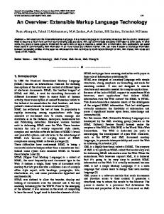
The difference between lengthening and widening plug-ins . . . . . . . . . . 27
3.1
An example of an arithmetic transformation. . . . . . . . . . . . . . . . . . 34
3.2
Checker board imposed over swirled vertical blue and red stripes . . . . . . 36
3.3
Some algebraic properties of Pan primitives . . . . . . . . . . . . . . . . . . 42
3.4
Effect of optimisations on frame rate at resolution of 320x200. . . . . . . . . 45
3.5
M2TH imports M1 which splices in declarations in M1TH. . . . . . . . . . 46
3.6
A comparison of three approaches to implementing DSLs . . . . . . . . . . 49
4.1
A monadic API for a typed lambda calculus with data types, pattern matching and let-expressions.
4.2
. . . . . . . . . . . . . . . . . . . . . . . . . . . . . 53
Two possible architectures for back-end plugins. 1) Dynamically loaded plug-ins 2) Plug-ins as stand-alone processes. . . . . . . . . . . . . . . . . . 55
4.3
An augmented display function that incorporates lifted images . . . . . . . 61
4.4
Creating the partial inner image . . . . . . . . . . . . . . . . . . . . . . . . 62
4.5
Creating a constant image and lift context . . . . . . . . . . . . . . . . . . . 63
4.6
The call graph of replaceIfLiftable
4.7
getLiftedImages . . . . . . . . . . . . . . . . . . . . . . . . . . . . . . . . . . 65
4.8
liftImageExpr . . . . . . . . . . . . . . . . . . . . . . . . . . . . . . . . . . . 66
4.9
The CPM monad . . . . . . . . . . . . . . . . . . . . . . . . . . . . . . . . . 68
. . . . . . . . . . . . . . . . . . . . . . . 64
4.10 The heart of the custom inlining pass
. . . . . . . . . . . . . . . . . . . . . 70
4.11 A dump of the Core code generated for stripes. . . . . . . . . . . . . . . . . 71 4.12 How the optimisation pipeline is scripted
. . . . . . . . . . . . . . . . . . . 71
4.13 Results for six effects containing liftable images . . . . . . . . . . . . . . . . 72 5.1
The initial module. It defines the data structure to represent the simple lambda calculus and an alpha conversion function. . . . . . . . . . . . . . . 80
5.2
The extension module. It extends the earlier data structure to represent let expression, defines an extra equation on the alpha conversion function and defines a new evaluation function. . . . . . . . . . . . . . . . . . . . . . . . . 81
5.3
Some helper functions that are also present in the extension module. . . . . 81
5.4a Preliminaries: the proxy type, Sat class and wrapper type . . . . . . . . . . 85 5.4b Initial component type and the base functionality class . . . . . . . . . . . . 85 5.4c Functionality instance . . . . . . . . . . . . . . . . . . . . . . . . . . . . . . 86 5.4d Unwrapping instance . . . . . . . . . . . . . . . . . . . . . . . . . . . . . . . 86 5.4e Capping classes, capping types and capping instances . . . . . . . . . . . . 86 5.4f Smart constructors . . . . . . . . . . . . . . . . . . . . . . . . . . . . . . . . 86 5.4g Regular declarations . . . . . . . . . . . . . . . . . . . . . . . . . . . . . . . 87 5.5a Module header and new component type . . . . . . . . . . . . . . . . . . . . 87 5.5b Instances for new equations on existing functions . . . . . . . . . . . . . . . 88 5.5c Functionality classes and explicit dictionary . . . . . . . . . . . . . . . . . . 88 5.5d Unwrapping instance . . . . . . . . . . . . . . . . . . . . . . . . . . . . . . . 88 5.5e Instances for new functions on all component types . . . . . . . . . . . . . . 89 5.5f Capping class, capping type and capping instances . . . . . . . . . . . . . . 89 5.5g Smart constructors . . . . . . . . . . . . . . . . . . . . . . . . . . . . . . . . 90 5.5h Regular declarations . . . . . . . . . . . . . . . . . . . . . . . . . . . . . . . 90 5.6h A diagram of two recursive dictionaries produced by AlphaCap instances on Exp and Exp 0. . . . . . . . . . . . . . . . . . . . . . . . . . . . . . . . . 91 5.7a Syntax of source language . . . . . . . . . . . . . . . . . . . . . . . . . . . . 93 5.7b Concrete symbols of the source language . . . . . . . . . . . . . . . . . . . . 95 5.7c Concrete symbols of the target language . . . . . . . . . . . . . . . . . . . . 96 5.8a Translation for open data declaration in the initial module (m = 0). . . . . 97 5.8b Translation for regular declarations in the mth module. . . . . . . . . . . . . 98 5.8c Translation for new equations on existing functions in the mth extension module. . . . . . . . . . . . . . . . . . . . . . . . . . . . . . . . . . . . . . . 98 5.8d Translation for extend data declaration and new function for the mth extension module. . . . . . . . . . . . . . . . . . . . . . . . . . . . . . . . . . . 99 5.8e Translation rules . . . . . . . . . . . . . . . . . . . . . . . . . . . . . . . . . 100 5.8f More translation rules . . . . . . . . . . . . . . . . . . . . . . . . . . . . . . 101 5.9
A mapping from symbols in the formal translation to identifiers in the running example. . . . . . . . . . . . . . . . . . . . . . . . . . . . . . . . . . 105
5.10 The F0 Alpha module implemented OCaml. . . . . . . . . . . . . . . . . . . 110 5.11 New functionality defined on the alpha function in OCaml module F1 Eval .111 5.12 Function eval defined on ordinary lambda expressions and the let extension in OCaml module F1 Eval. . . . . . . . . . . . . . . . . . . . . . . . . . . . 112 6.1
Rules for translation list comprehensions into more primitive expressions. . 120
6.2
The structure of a compiler for a typical functional language
. . . . . . . . 121
Chapter
1
Introduction
W
hile, in principle, it is possible to program any application in a Turing complete language some languages are better suited for certain tasks. That is, computational
possibility is not the only concern; we are also concerned with expressiveness, safety and efficiency, things which cannot always be provided adequately through software libraries. Within languages, expressiveness is provided through concise, elegant notations while safety is provided through either static checks, which are machine checked as opposed to being done by hand, or dynamic checks, which are tedious to manually implement. Efficiency can be provided through the agency of clever optimisation or run-time support for common implementation techniques. If we accept the aforementioned benefits, we are faced with a conundrum: despite their utility, creating new languages is expensive both in time and effort. In an effort to mitigate this reality it has been suggested that languages should be designed for extensibility. There are solid grounds for this approach. Established languages are more likely to have high quality implementations, a suite of useful libraries and good tool support such as IDEs, profilers and debuggers. There is also a higher likelihood that they benefit from a well-established programmer community that can be used as a resource to help train novices, give advanced help, and help improve and provide feedback on software. In this dissertation I tackle the issues arising from such a language implementation approach. I provide one answer to the question of how one should design a language and its implementation so that it can be extended with a minimum of extraneous effort. At its heart, this approach is concerned with reuse. The abstract space of solutions can be divided into halves: • Add language extension mechanisms to the language. Here we focus on language features that allow us to define new constructs that have equivalent functionality to constructs that would normally be built into the language standard. • Design the compiler to be extensible. There is always the option of extending a language by modifying the source code of an existing compiler. Yet for some compilers,
14
Chapter 1: Introduction
given their size and complexity, this can be impractical. Therefore, the basic thrust of this solution is to design extensibility into the compiler from the beginning. The primary focus of this dissertation is on a specific instance of the latter solution: a dynamically extensible compiler implementation, which I refer to henceforth as a plug-in compiler. As we shall see this variant has many features to recommend it over its statically extensible counterpart. Initially, I investigated a solution based on language extension mechanisms because, in many respects, it is more principled. The results of this research are included in this dissertation for two reasons. First, the techniques developed can be used with little modification in a plug-in compiler and second, the problems encountered during the execution of this approach are interesting in their own right and motivate the implementation of a plug-in compiler. Plug-in compilers provide the ability to extend languages without requiring the programmer to be intimately familiar with the source code of a particular compiler; all that is necessary is a familiarity with the exposed plug-in API. Consequently, the barriers to contribution are lowered. Simultaneously, the problem of code base forking is mitigated; with plug-ins it should no longer be necessary to fork the development tree of a compiler when testing experimental language extensions, only to be faced with the tediousness of integrating them back into the trunk once they have become well established. Back-end plug-ins also provide a means by which libraries can be distributed with their own optimisations; that is as active libraries.
1.1
Contributions of the dissertation
The main contributions of the dissertation are: • I show how Template Haskell, a compile-time meta-programming extension to Haskell, can be used to optimise user written code, thus allowing for domain specific optimisations to be written for embedded domain specific languages (EDSLs). Benchmarks for a specific EDSL, Pan, are provided. I also provide a comprehensive taxonomy of the problems with this approach. • I show how back-end plug-in support can be added to a compiler, GHC in our case, and how this functionality can be used to optimise user written code. This approach overcomes many of the shortcomings of the Template Haskell approach while introducing a few of its own. One of these is the loss of portability but a potential solution to this problem is investigated. • I provide a solution to the well-known expression problem in Haskell using type classes and existential types. The solution provides a way to extend data types and functions that operate on those data structures without modifying existing code while respecting separate compilation. Although a solution for Haskell has recently been proposed by L¨ oh and Hinze my solution works well in a plug-in environment. I
1.2. Structure of the dissertation
15
also suggest syntactic sugar for extending data types and provide a formal translation from a language augmented with the new syntax to Haskell. This translation could form the basis of an implementation. • The ability to write front-end plug-ins, which extend the syntax and semantics of a language, is added to a compiler for a Haskell-like language. The approach centres around providing plug-in points within and between each phase of the front-end of the compiler. This allows all aspects of the compiler’s functionality to be extended. As a case study I present a plug-in that adds list comprehensions to the language.
1.2
Structure of the dissertation
The rest of the dissertation is organised as follows. Background–Chapter 2. This chapter provides a more detailed motivation for the dissertation. It begins by covering the benefits of language features and the complexity of language implementations. I then present a survey of language extension mechanisms and the pros and cons of this approach. Most importantly the chapter provides an in depth motivation of plug-in compilers. Optimising EDSLs using Template Haskell–Chapter 3. Pan, an embedded domain specific language, is used as a vehicle to demonstrate an approach to domain specific optimisation using a meta-programming language called Template Haskell. This chapter provides the motivation for studying plug-in compilers. Plug-in optimisation–Chapter 4. This chapter discusses the addition of back-end plugins to a compiler. A plug-in optimisation that improves the quality of user-written Pan code is then presented along with benchmarks proving its efficacy. A real implementation exists for the Glasgow Haskell Compiler (GHC) and it is described. Also, the concept of plug-in DSLs is introduced. Such DSLs make writing plug-ins easier and improve the portability of a plug-in based approach. Extensible data types–Chapter 5. In order to write front-end plug-ins it is necessary to solve the expression problem. A novel solution is provided for the Haskell language. It involves the use of type classes, existential types and recursive dictionaries. A translation from a language augmented with syntactic sugar for extending data types to the Haskell language is also presented. A comparison with other well-known solutions to the expression problem in other languages is then made. Front-end plug-ins–Chapter 6. With the expression problem now solved I show how front-end plug-in support can be added to a compiler. The design centres around providing plug-in points between and within each phase of the compiler. I then present a simple, but powerful, plug-in that extends a simple functional programming language with list comprehensions. A real implementation exists in the form of
16
Chapter 1: Introduction
PHRaC, a small compiler written in Haskell, for a Haskell-like language. It makes
use of the techniques introduced in Chapter 5 and a discussion of the issues that arose during implementation is provided. Conclusion–Chapter 7. This chapter summarises the results of the dissertation.
1.3
Source code
The source code is available for all of the implementations described in this dissertation. The modifications made to GHC to provide back-end plug-in support are available from the pluggable-1-branch fork of the GHC CVS repository. They can be browsed online at: http://cvs.haskell.org/cgi-bin/cvsweb.cgi/fptools/ To download and build the pluggable GHC compiler see the instructions at: http://www.haskell.org/ghc/docs/latest/html/building/index.html The back-end plug-in for the Pan DSL, the implementation of PHRaC and the corresponding list comprehension front-end plug-in are all available as darcs 1 repositories at: http://www.cse.unsw.edu.au/∼sseefried/darcs/ The names for these projects are plugpan, plug phrac and listcomp phrac plugin respectively.
1
The revision control system, darcs, can be found at http://abridgegame.org/darcs/.
Chapter
2
Background
T
his chapter provides the motivation for choosing a plug-in architecture to build extensible compilers. In turn, they may be used to extend languages or implement
domain specific languages (DSLs). The work is founded upon the assumption that more programmers would try their hand at language design were it not for the high barrier to entry. I claim, as others do [82], that writing new languages is an expensive task both in time and effort. The difficulty of language implementation motivates an approach to language construction based on reuse. I go on to describe two ways in which language infrastructure can be reused. The first way, via language extension features, relies on a sufficiently powerful host language within which it is possible to define terms which adequately embody new language features. The second way is to extend a compiler. The efficacy of this approach depends greatly on the manner in which the compiler is designed. I argue that a plug-in compiler, a compiler which loads and runs code at program compile time, provides a convenient and powerful mechanism for language extension.
2.1
Why extend languages?
A Turing complete language can express any computable function; thus, with adequate support for I/O, it’s possible to do anything in any programming language. However, computational possibility is not the only concern. Languages are also prized for their conciseness, safety, efficiency, and reasoning properties (among other things). Sometimes libraries can only offer so much and new language features become increasingly attractive. A brief summary is provided below. • Conciseness. Concise notations can remove the need to write verbose, idiomatic code. This leads to a reduction in the number of lines that need to be written to express a program. • Safety. Safety relates to static or dynamic checks upon programs to ensure that they do not perform certain types of unwanted behaviour. Features such as type systems, exceptions, garbage collection and assertions all fall under the umbrella of
18
Chapter 2: Background
safety. A domain specific language can further enhance safety by providing checks tailored to a particular application area. • Efficiency. Static guarantees can often be made about code and sometimes lead to optimisation opportunities. Also, support can be provided by the run-time system for efficient programming of certain applications. e.g. light-weight threads for concurrency. • Reasoning. Some languages1 have elegant algebraic properties which can be exploited by programmers wishing to prove the correctness of their programs. These properties can also be used to improve the efficiency of code. Developing languages from scratch can be a daunting undertaking. Defining their semantics and implementing them constitute a large part of the difficulty. It can be years until a fully fledged implementation for a language is available. In this section we explain these difficulties in detail, as well as providing further evidence in favour of language reuse.
2.1.1
The complexity of languages
New languages tend to evolve from older ones, a form of intellectual reuse. In the process they may acquire features which may or may not interact well with existing features. Making these new features “play well together” with existing ones constitutes one of the main challenges of programming language design. A precise formal semantics for language features provides a powerful tool for designing and checking the consistency of languages but requires significant investment and is often not undertaken for this reason. The complexity of languages is reflected in the fact that some in wide use today contain semantic inconsistencies, or at least an inelegant semantics. For instance, Javascript is well-known for its abundance of “gotchas” [24]. While the semantics of the language has been defined [30] and a typing system has been developed for it [92], it is clear that more thought should have been put into whether each feature was sufficiently well-defined before being added to the language. A good indication of the semantic complexity of a language is to measure the size of the language standard. These can easily run into the hundreds of pages2 [6, 7]. The current state of the art is that such standards are written almost exclusively in natural language. Despite extensive research nearly all popular non-trivial languages have resisted mathematical formalisation due to their sheer complexity, although it would be remiss to omit a mention of the heroic work done in partially formalising Standard ML [69]. Clearly, the sheer effort required to define a language’s semantics is a strong point in favour of their reuse. Also, language design can be seen as a form of intellectual reuse, an exercise in selecting the best features from earlier languages and combining them with novel additions. As far as possible this should also be an exercise in software reuse. 1
Cryptol [1] is an example. R5RS, the standards document for Scheme, is a notable exception running for only fifty pages. Much effort was expended in reducing it to this size. 2
2.1. Why extend languages?
2.1.2
19
The complexity of implementations
Implementing a language to a level where it can be used productively can take many months if not years. Although interpreters are, in general, easier to write than compilers, either form of implementation requires a significant amount of effort. Both compilers and interpreters must lex, parse, and analyse source code. The first two of these phases are probably the most well understood. Lexing is usually done using a lexer generator tool which generates code that encode a deterministic finite state automata (DFA) to perform the task. Parsing, on the other hand, can be done using a number of different algorithms. Each algorithm trades speed and/or space for expressiveness or vice versa to some extent3 . There is a lot of compiler infrastructure surrounding the parser such as the definition of the representation data structure (often an abstract syntax tree), a symbol table, and libraries for name generation, error reporting and graph manipulation. After parsing comes analysis. This involves checking for errors in the source which cannot be done during parsing, such as checking the scope of variables, and more sophisticated analyses such as type checking, and data flow analysis. And this is only the front-end. Interpreters must now execute the code directly while compilers must optimise and generate code. Optimisations form a large part of modern compilers and are often sophisticated. As a language develops it is this section of the compiler more than any other that is likely to grow in size and complexity. This phase of the compiler can also be divided into sub-phases in which the program is translated into one or more intermediate forms upon which certain optimisations are particularly effective or easy to specify. e.g. Static Single Assignment (SSA) form [25] or Administrative Normal Form (ANF) [23]. This leaves only code generation. There are several factors which complicate this phase of the compiler. First, there may be multiple architectures that need to be targeted. The disparate nature of machines means that it is often difficult if not impossible to share code generation routines; each platform must be targeted in isolation. Also, many hardware architectures are designed with simplicity of processor design in mind. This often means that functionality that would have been implemented in hardware in the past must now be implemented in software. Clearly, there is strong evidence that implementing compilers is a lengthy and ongoing task. Fortunately, the need for reuse in the area of compiler implementation is well recognised and has received much attention. One way in which the effort of a compiler implementation is mitigated is through the use of compiler construction tools. Parser generators are perhaps the most well-known instance of compiler construction tools. They save the work of writing parsers by hand and have been in use for over two decades. They process lexical tokens and specify the order in which they should be combined into data structures which represent the structure of the source code. But this is all most of them do. It is still up to the programmer to attach an action to each symbol 3
At the fast but inexpressive end of the spectrum are recursive decent and LL parsers. At the other end are LR and Earley parsers, the latter of which can parse any context free grammar but has a cubic time complexity.
20
Chapter 2: Background
of the grammar. Such an action may, for instance, take two expressions and an operator and combine them into an aggregate expression. Other compiler construction tools focus on different phases of the compiler. Attribute grammars can be used to generate and synthesise values in the abstract syntax tree. They can be used to write program analyses and even do code generation. Another tool, Stratego/XT [98, 97], provides a language for writing transformations on abstract syntax trees using the paradigm of rewriting strategies. There are also tools that can create large parts or even all of a programming environment. Among these are (BEG) [35], a back-end generator that translates declarative specifications to code-generators, ELI [44], which can be used to construct an entire compiler and Centaur [18] which can create a programming language environment (editor, compiler, debugger, etc) from a formal specification of a language.
2.1.3
Programming environments and communities
A fully fledged language does not merely consist of an implementation. It is surrounded by a suite of useful tools, often called the programming environment and a community of programmers that use the language. The case for re-use is about more than just the effort required to write a compiler. Among the tools that can improve the productivity of programmers are profilers, debuggers, Integrated Development Environments (IDEs), and syntax highlighting packages. There is likely to be a high degree of correlation between how widely used a language is and how well-developed such tools are4 . Thus, in choosing to use a particular language, a programmer also benefits from the inheritance of its programming environment. However, It should be kept in mind that an extensible language will require extensible tools. One should also not underestimate the usefulness of a large (and often highly skilled) programming community. They often take years to form but once present are a considerable resource which can be drawn upon for support of one’s own software projects. They also provide a platform upon which the future development of the language can rest. When dealing with the complexities of language semantics it can be of enormous benefit to have a large body of interested and intelligent people check the soundness of one’s ideas. Also, such communities can only form around languages which have demonstrated their utility and are likely to continue being relevant into the foreseeable future. There is only a slim likelihood that a one-off DSL will develop a rich community around it.
2.2
What sorts of extension are we interested in?
Before going on to discuss how languages may be extended a moment should be taken to discuss the kinds of extension this dissertation is concerned with. 4
Oliver Steele believes that languages tend to become either tool focused or feature focused [87]. This does not contradict the relationship I postulated above as he is only concerned with well-established languages. Even in feature focused languages there will be some tool support.
2.3. Methods of language extension
21
I do not use the term extension in the sense in which it can be used in other fields (such as language semantics); our extensions do not necessarily increase the expressiveness of the language, they may simply make them less verbose, more elegant, and/or safer to use. I regard as extensions things such as new control flow constructs, additions to the typing system, and syntactic sugar. Extensions can be divided into three broad categories: expressiveness, safety and efficiency. Expressiveness extensions increase the capabilities of a language, often allowing something that would have been idiomatic and verbose to be concisely captured in a suitable syntax. Safety extensions improve the detection of undesirable behaviour in programs or, as in the case of garbage collection method of memory management, remove the need to consider certain behaviours at all. Efficiency extensions are concerned with improving the quality of generated code.
2.3
Methods of language extension
Accepting the arguments for reuse the language designer is now faced with the problem of how to achieve it. In this section I provide a survey of the ways in which a language can be extended. There are three broad categories into which one can divide the methods of language extension: language features for extensions, henceforth known as extension features, extensible implementations and external extension (which is not considered in this dissertation). These methods of language extension are not mutually exclusive. There is nothing stopping a language designer from using extension features and extending the compiler. In fact a combination of the two may well be the most prudent path.
2.3.1
External extension
This method of extension covers pre- and post-processors. Pre-processors take source code and re-write them to target an existing compiler or interpreter, while post-processors take the output from an existing compiler and transform it some way. Pre-processing is a popular way of extending languages but can end up duplicating a lot of work. The parser for the pre-processor is often only a small extension to the parser for the target language. Naturally, it is possible to find the parser for the target compiler/interpreter and extend that but this means that the programmer must keep this extension synchronised with the target language. Also, if one wishes to include static analysis done by the target compiler/interpreter this must be painstakingly recreated in the pre-processor. Usually, this is omitted which leads to incomprehensible error messages emitted by the target language compiler when errors are made in the source code to be pre-processed. Pre-processors are powerful but brute force approach to language extension. We do not consider them further in this dissertation.
22
Chapter 2: Background
2.3.2
Extension features
At a glance familiar features such as function definitions and data type declarations do not merit the status of extension feature but a closer inspection reveals no reason why they should be excluded. The essence of an extension feature is that it allows a programmer to imbue a language entity with a semantics expressible using existing language entities. Macros, inheritance, aspects, higher order functions, reflection, and meta-programming can all be perceived in this light. However, we focus on the more powerful features: macros and meta-programming. Macro systems have been part of LISP and Scheme for some time. They provide a powerful mechanism for defining new syntactic entities in terms of existing ones. In general, one of the major drawbacks they have is that names used inside the definition can be bound to incorrect names in the local scope. Scheme introduced the notion of hygienic macros [57] to solve this problem; they ensure that any free variables are looked up in the scope of the macro definition not where it was used. Meta-programming is another compelling choice for extending languages. This programming technique was first studied by Smith [86] and then by others in the Lisp and Scheme communities [40, 104, 28, 54]. During this period notions of name generation and quasi-quotation were refined. Sheard, Taha and Pasalic [90, 91, 85, 76] introduced reflection into a strongly typed setting thus further increasing the safety of this powerful programming technique. Features such as extensible syntax and GHC’s rewrite rules fall under the umbrella of meta-programming. Sometimes extension features are entirely adequate for defining the primitive constructs of an entire language. That is, it is possible to define distinct, syntactic entities that have a one-to-one correspondence with semantics of entities in another language. Embedded domain specific languages (EDSLs) are implemented as libraries in precisely this manner. The richer the host language the more opportunity there is for this technique to be used5 . Meta-programming does have its limitations. It is constrained by the degree to which one chooses safety over power. Also, the richer a language is syntactically, the more tedious it is to write transformations using meta-programming since many syntactic cases need to be considered. Chapter 3 of this dissertation is concerned with the application of a compile-time metaprogramming language, Template Haskell, to an EDSL for image synthesis known as Pan [32].
2.3.3
Extending the compiler
At its simplest this method of extension involves modifying the source code of a compiler, so-called static compiler extension. However, a compiler can also be extended at run-time via plug-ins; this is called dynamic compiler extension. For this to be an effective method of reuse the compiler needs to be designed for 5
Examples of EDSLs are abundant and include Pan [32], HaXML [103], Fran [31, 34, 22], FranTk [83], FAL [49], Haskore [51], and Yampa [50, 71].
23
2.4. Plug-in compilers
extensibility. Extensibility depends on at least the following factors: the implementation language, orthogonality of the implementation, coupling between modules, and the data structures chosen. The choice of implementation language is probably the most important of all. Features such as inheritance and extensible data structures have a clear utility. The continuous scale of extensible implementations can be partitioned into three categories: rigid, statically extensible, and dynamically extensible. Each is an evolution of the one before. In this dissertation the term rigid is used to describe language implementations that are hard to extend (for whatever reason). Although such implementations are often monolithic, I use the term monolithic to describe applications which are compiled to a single executable and do not load in plug-ins. A monolithic compiler could nevertheless be quite extensible if designed well. From rigidity to dynamic extensibility If a programmer wishes to extend a language there is nothing stopping them from modifying the source code of a compiler. As has already been stated, this could be difficult. Production quality compilers are often hundreds of thousands of lines of code, composed of modules written by many people and of differing quality. But this is not the only hindrance. As soon as the modifications have been made, and assuming your extension is not accepted by the mainstream, the implementer has locked themselves into one of two possibilities: either the new version of the compiler must be developed in isolation from the old version, never to be merged, or worse, new developments in the old version must be periodically and tediously merged into the new version. Despite these difficulties the lack of alternatives often drives people to extend languages in just this way. A statically extensible compiler addresses the problem of badly designed, inextensible code. Examples of such compilers include Polyglot
6
[72], Pizza [108] and Cetus [64].
They are designed with extension in mind from the beginning. If designed correctly the problem of keeping variants in step with the original code base is ameliorated. However, different versions of compilers built in this way must still be separately installed and used on one’s system. Only a small step in functionality separates statically extensible compilers from their dynamically extensible counterparts known as plug-in compilers: the ability to load and run plug-ins at run-time. However, this small boost in functionality opens up a large array of opportunities not possible before. Describing these opportunities is the focus of the next section.
2.4
Plug-in compilers
Plug-in compilers are the central focus of this dissertation. Puzzlingly, only minimal attention [82, 13, 36, 106] has been paid to the idea of a plug-in compiler even though the utility of plug-ins is widely accepted in other applications. These include Firefox [2], the GIMP [9], Adobe Photoshop, Winamp [10], and Emacs [3]. The essential idea is to 6
abc [17], a compiler for AspectJ, is an extension of this.
24
Chapter 2: Background
expose the internals of the compiler through a rigorously defined API and to provide entry points or hooks into the phases of the compiler. User-written plug-ins can be compiled separately, dynamically loaded at compiler run-time (i.e. program compile-time) and run as part of the compiler. However, there are frameworks which provide functionality that overlaps to high degree with that of plug-in compilers. An example of this is the CoSy compiler framework [15, 39] which provides a principled way to write and combine stand-alone compiler units into sophisticated compilers. (It is particularly useful for writing complex optimisation suites.) Its architecture centers around engines which have access to a central, shared intermediate representation of the program. The engines can be composed, and ordered using an Engine Description Language (EDL). More about CoSy and its similarity to the work presented in this dissertation is discussed in Chapter 4.
2.4.1
Advantages
Plug-ins can fundamentally change the way in which compilers are developed and maintained. The next few sections explain some of the manifold benefits of this approach to compiler construction.
Complexity One of the most daunting aspects of studying the source code for a compiler is its sheer size. A plug-in compiler encourages the development of a minimal core compiler that is then extended with functionality via plug-ins. This leads to an implementation which is loosely coupled, in which module boundaries more accurately reflect functional boundaries. Conversely, the current state of the art is beset by the problem of cross-cutting features. For instance, the implementation of syntactic sugar in a traditional compiler cuts across the lexing, parsing, analysis, type checking and sometimes even the code generation phases of the compiler. Although it is too early to say with certainty, the ability to separate the core compiler from a larger, fully-functional language implementation may lead to an application that is less complex and easier to understand. This in turn could reduce development times and improve maintainability.
Safety and Verification Plug-ins encourage modularity. This reduces the chances that compiler bugs remain undetected by making it possible to test the compiler in layers. The core compiler can be thoroughly tested before plug-ins are even considered. A plug-in architecture may be of some assistance in achieving the dream of compiler verification. Much of the difficulty associated with proving correctness is that there has simply been too much extraneous detail present in the compiler. By moving some of this detail out into plug-ins, the process of verification may be simplified.
2.4. Plug-in compilers
25
Distribution Plug-ins allow language extensions to be distributed as libraries; hence they can be used as a method of implementing active libraries [96, 26, 95]. Not only does this make their distribution easier, it also fundamentally changes the marketability of extensions. For instance, consider the development of a new optimisation technique. The current state of affairs is that an optimisation is either included in a compiler or not at all. Optimisation writers must show that their techniques are generally applicable, that they improve the performance of a wide range of programs. If not, they cannot go in the compiler because they may slow down existing programs. However, this misses the fact that they may be particularly effective on a specific set of programs. Peyton Jones et al. [78] eloquently phrases this: Compiler optimisations are like therapeutic drugs. Some, like antibiotics, are effective on many programs; such optimisations tend to be built into a compiler. Others are targeted at particular “diseases”, on which they are devastatingly effective, but have no effect at all on most other programs. Plug-ins allow such “niche market” optimisations to exist and perhaps even flourish. They can be used precisely where they are useful. A large collection of only-sometimesused optimisations leads to the idea of profile driven optimisation in which aggressive profiling is used to decide which optimisations are used on a particular piece of code. This is similar to the technique used in the FFTW library [41]. A similar reasoning applies to language extensions, purely syntactic or otherwise. Features must be generally useful and more importantly non-disruptive to the entire language community if they are to go into a compiler. At the moment such non-standard extensions are baked into the compiler and enabled with command-line flags. However, having little used extensions remain inside the compiler bloats it unnecessarily. It is semantically cleaner to realise them as plug-ins. Development A language succeeds or fails based on whether it can acquire and sustain the attention of a large group of programmers. Plug-in compilers motivate development on a language by lowering the barrier to entry. No longer is it necessary to understand the intricate details of the inside of the entire compiler in order to write extensions. In this way the work of maintaining a language’s vibrancy is distributed more evenly among its users7 . This can only help improve its chances of survival. Plug-ins can also be used to help develop the compiler via a process of bootstrapping. Plug-ins can be used to create DSLs useful for writing key phases of the compiler such as parsing, type checking or code generation. These DSLs can then be used inside the core 7
And means that the probability of a “bus error” is reduced. “Bus error” is a comic term describing the situation where an application’s development is halted due to unfortunate circumstances befalling one of its key maintainers.
26
Chapter 2: Background
compiler source code. Henceforth we call such languages plug-in DSLs. (In Section 2.4.3 we see how plug-in DSLs can be used to mitigate a common criticism of plug-in compilers.) Maintenance We have already mentioned that plug-in compilers encourage stricter interfaces which, in turn, encourages modularity. This is a simple consequence of the fact that it is hard to change the exposed API. Hence, increased attention must be paid to the interface. However, a plug-in compiler also benefits the development of and maintenance of language variants; language implementations that add a key feature such as concurrency, parallelism, or bounds checking to an existing language. Plug-in compilers should allow such variants to stay in step with each other. This point is illustrated by considering the bounds checking extension for the C language8 . It is implemented for the GNU Compiler Collection (GCC) as a collection of patches, one for each version of the compiler. The maintenance of this extension would be alleviated if it were possible to distribute it as a plug-in. Flexibility Plug-in compilers need not even be restricted to one language. A core compiler could implement a small, but rich intermediate language suitable for implementing the features of a range of different languages.
2.4.2
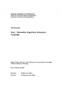
Classification and applications of plug-ins
In this dissertation compiler plug-ins are classified in two ways: front-end vs. back-end and lengthening vs. widening. A front-end plug-in is primarily concerned with extending expressiveness and safety of languages while a back-end plug-in is concerned with either optimisation or code generation. A widening plug-in is one which adds to the functionality of existing phases of the compiler. A plug-in which added new syntactic sugar would be such a plug-in. A lengthening plug-in introduces a new phase to the compiler. For instance, it may translate one intermediate language into a second, new intermediate language, perform optimisations on that representation and then translate it back into the old representation. Lengthening plug-in points exist between compiler phases; they take the output of the previous phase and produce the input for the following one. Figure 2.1 presents the classifications graphically. Plug-ins for expressiveness and safety Both the expressiveness and the safety features of a language are implemented within the front-end of a compiler. Accordingly these facets of a language are extended via front-end 8
The patches are available at http://gcc.gnu.org/extensions.html
27
2.4. Plug-in compilers ...
Phase n
Widening plug−in
Lengthening plug−in
Phase n+1
...
Figure 2.1: The difference between lengthening and widening plug-ins plug-ins. The applications of these plug-ins are limited only by the language designers imagination. A sample of the sorts of things that can be done are as follows: • Syntactic sugar. The term syntactic sugar describes additions to the syntax of a language which do not affect its expressiveness but make it “sweeter” for humans to use. Such syntax is “desugared” into existing language constructs. Such a plug-in involves extending the parser, extending the abstract syntax, and the addition of a desugaring phase. We consider just such a plug-in in Chapter 6. • New language features. This plug-in is identical to the one above except that it genuinely increases the expressiveness of the language. It may need to be used in conjunction with a back-end plug-in to generate new forms of code. • Error messages. This form of plug-in extends the language with custom error messages, perhaps for, but not limited to, domain specific syntactic extensions. • New safety checks. These can be either static or dynamic. Front-end plug-ins can be used to implement static checks. Examples include new kinds of static analysis and checks for erroneous conditions not covered by the type system of the language being extended. Back-end plug-ins can be used to instrument generated code with run-time checks. Plug-ins for optimisation and code-generation Back-end plug-ins can be used to provide custom optimisations for DSLs and, in particular, EDSLs. They can also be provided for libraries making them into active libraries [96, 26, 95]. In Chapter 4 we consider plug-in optimisations for the Pan EDSL [32].
28
Chapter 2: Background
2.4.3
Common criticisms of plug-in compilers
In this section I respond to some common criticisms of plug-in compilers. Portability Robinson states in a paper [82] on the economics of compiler optimisations: [Writing plug-ins] requires detailed knowledge of the compiler’s internal representation of a program, which is often strewn with decorations that must be maintained for the sake of other optimizations. This valid concern can be mitigated by careful attention to the API that is exposed. However, an even more effective way is to re-introduce portability through the implementation of DSLs for writing plug-ins. Once it has become standard practice to implement extensions via these DSLs the same forces—both social and technical—that cause widely used languages to be standardised will inevitably extend themselves to these DSLs. As an example, the CoSy compiler framework has a number of DSLs that are used to write its compiler units. EDL has already been mentioned. It can be used to specify dependencies between compiler units. There is also a structure definition language called fSDL that can be used to specify visibility, side effects and data structures used by the compiler units, that is, the interface between compiler units. This greatly clarifies the relationship between compiler units. Language Standards The second common criticism of plug-in compilers is one of language volatility. The fear is that the barrier to the modification of languages will be so low that language variants will flourish to such an extent that the notion of language standards will suffer. I respond to this criticism in two ways. First, the choice of more language variants in no way diminishes any of the benefits of standardised languages. When the development of an application in a standard variant of a language is perceived to be of great enough value it can still occur. Second, there is a perception in the programming community that some language standards have become too rigid. This perception is reinforced by examining the time between the release of versions of well-known language standards. For instance, there was a nine year gap between the C89 [5] and C99 [6] standards. Rather than damaging the notion of standards I envision that plug-ins will induce a hierarchy of rigidity in standards. The most rigid standard would be the core language. Presumably after that would come a language with standard syntactic sugar added, followed by various user extensions to the language, and so on. It would be up to users of the language and its extensions to decide how rigid they required their standards to be. In turn this may mean that the success or failure of a language extension is determined by natural selection (of its users), offering a refreshing alternative to the often criticised style of development known as “design by committee”.
2.5. Meta-programming vs. plug-in compilers
2.4.4
29
Limitations of plug-in compilers
It is tempting to think that plug-in compilers allow one to extend languages in arbitrary ways. Sadly this is not the case. The utility of plug-ins depends on two things: how orthogonal the extensions are to existing features and how well the compiler is modularised. For instance, a programmer may discover that a facet of a language is really a special case of a much more general and powerful formalism. This frequently occurs when extending the type systems of functional programming languages. This is an example of a non-orthogonal change and in this situation a plug-in compiler is not much help. The only sensible approach is to refactor the design of the compiler. The focus in this dissertation is on extensions that can be made within the existing framework of a compiler.
2.5
Meta-programming vs. plug-in compilers
Meta-programming is a relatively principled approach to language extension. However, meta-programming languages are often not expressive enough to perform the kinds of extensions we want. On the other hand, approaching the problem using plug-ins is more powerful but not nearly as safe. Safety can be increased by carefully choosing which portions of the compiler to expose. The two approaches are complementary. Both approaches converge on an optimum point which has both adequate expressiveness and safety. The development of metaprogramming languages moves from low expressiveness but high safety towards the optimum while the development of plug-in compilers moves from a position of (perhaps excessive) expressiveness and low safety toward the optimum. However, the effort required to add features to a meta-programming language is greater than that required to expose less of a plug-in compiler via the API. Ultimately, the techniques used in plug-in compilers should be used to inform the design of meta-programming languages. Chapter 3 is an experiment in the application of meta-programming for the optimisation of an EDSL. The chapter concludes with several reasons why the meta-programming language used, Template Haskell, is inadequate for the task. This provides the motivation to switch to the plug-in compiler solution which is described in the remaining chapters of the dissertation.
2.6
Why Haskell?
The results contained within this dissertation can be implemented in any language with sufficient expressiveness. However, almost all code that appears in the remainder will be written in Haskell. The reasons for this are: • Haskell has excellent support for data structures. They are easy to construct and in conjunction with Haskell’s support for pattern matching it is easy to de-construct and manipulate them. Memory allocation and memory layout are handled entirely
30
Chapter 2: Background
by the language so that the programmer is shielded from space leaks and complicated pointer manipulation. Since a large portion of any compiler is concerned with the handling of abstract syntax trees Haskell significantly simplifies their implementation. Languages from the ML family confer the same benefit. • In Chapter 3, Template Haskell is used to optimise an embedded domain specific language. This language is the culmination of many years of research into functional meta-programming languages [90, 91, 84, 85]. Similar in power to C++ templates [94] it is nevertheless more principled with support for quasi-quotation, automatic handling of scoping and name generation, and the algebraic manipulation of code. Even though I abandon the meta-programming approach after Chapter 3, techniques such as the algebraic manipulation of abstract syntax and the use of monadic code to adequately handle name generation, can be used in plug-ins. • As mentioned earlier, some domain specific languages can be embedded as libraries within another, albeit without the advantages of domain specific optimisations and error messages. The more expressive the host language the more applicable this technique becomes. Haskell’s syntactic control features, laziness, higher order functions and rich type system make it an ideal candidate for EDSL implementation. These features will be further discussed in Section 3.1.1.
2.7
Further related work
Each chapter of this dissertation is self-contained in the sense that they draw on relatively disparate areas of programming language research. Hence, the related work shall be deferred until the end of each respective chapter.
Chapter
3
Optimising Embedded DSLs with Template Haskell
I
n contrast to the remainder of the dissertation this chapter attacks the problem of language reuse using a language extension feature, specifically, compile-time meta-
programming. The primary purpose of this chapter is to motivate the plug-in compiler approach by highlighting the problems encountered using a state-of-the-art metaprogramming language, Template Haskell, on an embedded domain specific language called Pan. Template Haskell is a sophisticated language incorporating many of the best design choices of earlier meta-programming languages—such as support for quasi-quotation, static and dynamic scoping and convenient manipulation of abstract syntax—and improving upon them with features such as staged static typing. This approach transforms user-written code according to its syntactic structure. The key idea is to represent code as a data structure (preferably an abstract syntax tree), manipulate this data so that it represents equivalent but faster code, and finally turn this data back into code. It can be thought of as a principled or augmented form of pre-processing. Language support is provided for generation of new symbols, static and dynamic scoping, reification, and a novel staged type-checking algorithm (explained further in Section 3.1.2). Thus, much of the tediousness of writing pre-processors is removed while additional safety is introduced. Despite Template Haskell’s sophistication, it falls short of being a suitable language for library/EDSL optimisation. It turns out that an advantage of meta-programming over plug-ins, namely its compiler independence, is also a problem. Meta-programs have fairly limited access to internal information, which can lead to poor error messages and difficulty in implementing safety features. Of course, we could design meta-programming languages that expose more information, but then we raise similar questions to those raised when designing plug-in compilers. Conversely, this indicates that meta-programming can inform the design of APIs for plug-in compilers and maybe DSLs for compiler plug-ins, something we will come back to in Chapter 4. The chapter is organised as follows. We begin with a discussion of why Haskell is
32
Chapter 3: Optimising Embedded DSLs with Template Haskell
a good host language for EDSLs and follow this with a short introduction to Template Haskell describing how it is used and what features make it state-of-the-art. We then introduce the Pan EDSL—which is considered in both this chapter and the subsequent one on plug-in optimisations—and my implementation of it, PanTHeon. We then describe the implementation of three different source level transformations that were implemented in PanTHeon. This is followed by two sets of benchmarks. One proves their efficacy by comparing optimised code against unoptimised code while the other compares PanTHeon against an earlier implementation of Pan by its designers. An in depth discussion of my experience with Template Haskell follows, describing areas where it falls short of what is required. This provides the background to motivate the plug-in compiler approach. In summary the contributions of the chapter are: • The efficacy of compile-time meta-programming is demonstrated on a realistically sized domain specific language, Pan. Three different optimisation techniques are introduced and demonstrated. Benchmarks are provided. • Drawbacks of the compile-time meta-programming approach are identified an explained. • This provides the motivation for a plug-in compiler based approach to providing domain specific optimisations.
3.1
Haskell for EDSLs and meta-programming
Before introducing the Pan DSL we focus upon the features of Haskell that make it suitable for implementing EDSLs and then introduce Template Haskell, a compile-time metaprogramming extension implemented in the Glasgow Haskell Compiler (GHC).
3.1.1
Haskell: a good host language for EDSLs
Haskell has a number of features that make it ideal for implementing EDSLs. Laziness Laziness can be used to provide the same behaviour as control flow constructs in other languages. For instance consider what would happen in the following code if the if-thenelse construct was strict: f x = if x == 0 then 1 else f (x − 1). Using laziness, one can define a function, ifF , in Haskell that provides the required behaviour. ifF :: Bool → a → a → a ifF True thenPart
= thenPart
ifF False elsePart
= elsePart
3.1. Haskell for EDSLs and meta-programming
33
Syntax control Haskell has declarations that can change the precedence, fixity and associativity of user defined functions. This allows the syntax of the EDSL to more closely resemble that of a real language. For instance Haskell defines + and ∗ to be left associative with the former having a lower precedence than the latter. This is done with the following declaration in the Prelude. infixl 7 ∗ infixl 6 +, − This means that expressions such as 2 ∗ 3 + 7 parse and evaluate to the correct value, 13. Unlike other languages this is defined in Haskell’s libraries, not its compiler. Higher order functions Higher order functions allow powerful combining forms to be defined that offer the same power as built-in operators in other languages. Rich type system Haskell has a rich type system that allows new, mutually recursive algebraic data types to be defined. Used carefully one can disallow certain expressions in the EDSL simply by making sure they lead to type errors in Haskell. For instance, in a linear algebra setting we can make sure that only vectors can be added to points by defining types and functions as follows. newtype Vector = Vec (Int, Int) newtype Point = Pt (Int, Int) plus :: Vec → Pt → Pt (Vec (dx , dy)) ‘plus‘ (Pt (x , y)) = Pt (x + dx , y + dy)
3.1.2
Compile-time meta-programming using Template Haskell
This section introduces Template Haskell. We start by showing how a useful algebraic transformation can be implemented. Since the optimisations of PanTHeon are treated more than adequately in the rest of the chapter we focus on a useful transformation in a well-known domain: linear algebra. A basic result of linear algebra is that an n × n matrix, M , multiplied by its inverse, M −1 ,
is equal to the identity matrix, I. This is just the sort of property that we cannot
expect most compilers to optimise away, due to the domain-specific knowledge that is required to perform such an optimisation. Consider an expression m ∗ inverse m where m is a matrix. (The precise details of how matrices are implemented is immaterial.) In order to simplify this expression it must first be converted from code into a data structure via a process known as reification [40].
34
Chapter 3: Optimising Embedded DSLs with Template Haskell
rmMatByInverse (InfixE (Just ’m) ’GHC .Num.∗ (Just (AppE ’inverse ’m))) = VarE (mkName ”identity”) rmMatByInverse (LamE pats exp) = LamE pats (rmMatByInverse exp) rmMatByInverse (AppE exp exp � ) = AppE (rmMatByInverse exp) (rmMatByInverse exp � ) rmMatByInverse exp = exp
Figure 3.1: An example of an arithmetic transformation. Once we have verified that this data structure matches the pattern �matrix� ∗ inverse �matrix� we can replace it with the data structure that represents identity. We then need to convert the data structure back into code, via a process known as reflection [86]. This is also known, particularly in Template Haskell, as splicing. The expression, m ∗ inverse m ∗ n is reified into an algebraic data type. The transformation of this expression is then simple. A new data structure is created which represents identity ∗ n and spliced. We now show how this is achieved using Template Haskell on a (rather contrived) lambda expression with body equal to m ∗ inverse m ∗ n. exp mat = [| λ m n → m ∗ inverse m ∗ n |] exp mat makes use of the quasi-quote notation of Template Haskell, denoted by the [| and |] brackets. These brackets reify code within. Figure 3.1 presents the function rmMatByInverse which removes the redundancy in the reified expression. The first case does the real work; it matches against infix expressions of the form �matrix� ∗ inverse �matrix� and returns identity, while the second and third (after matching against expressions of the form lambda p → e and f a respectively) recursively apply to sub-expressions. (Note that we have only presented the cases necessary to transform exp mat.) Template Haskell’s splicing operator, $(. . . ), runs meta-programs and converts the resulting data structure back to code. In our case the expression $(rmMatByInverse exp mat) evaluates to the code λ m n → n at compile-time. This is a key aspect of our approach; by using a language which is restricted to compile-time meta-computation we guarantee that there is no run-time overhead in the code generated. Features of Template Haskell Template Haskell has a number of features that make it particularly well suited to generating and manipulating programs. First, it respects static scoping. The original paper on Template Haskell presents an example of a meta-program that mimics the behaviour of C’s printf function by generating
3.2. Introduction to the Pan DSL
35
a function which takes the required arguments (of required types) as parameters. It is defined as follows: data Format = D | S | L String printf :: String → Q Exp printf s = gen (parse s) [| ”” |] gen :: [Format] → Q Exp → Q Exp gen [] x = x gen (D : xs) x = [| λ n → $(gen xs [| $x + + show n |]) |] gen (S : xs) x = [| λ s → $(gen xs [| $x + + s |]) |] gen (L s : xs) x = gen xs [| $x + + $(lift s) |] The n and s bound by lambdas in the third and fourth equations of gen are used within the nested quasi quotes. Had a different variable name been used a scoping error would have been signalled by the compiler. Second, Template Haskell maintains type safety through staged typing. Traditionally, a program is type checked, compiled and then executed. However, we now have execution of code generators occurring at compile-time. In contrast to MetaML, which type-checks all programs before code generation, Template Haskell chooses to interleave type checking with generation. First, the meta-program is type checked at the abstract syntax level. This is, it is determined whether the value produced will be of the type of a representation of a declaration, expression, etc. Whether the program represented type checks or not is another question. The meta-program is then executed and the final program type checked as if the programmer had written it in the first place. Third, quasi-quotation and nested splicing provide a convenient way to generate programs. Finally, programs can be reified and manipulated using ordinary algebraic data types. Without this capability transformations of the kind demonstrated above could not be done. Also, there are times when the quasi-quote notation is not adequate to generate expressions. For instance, this occurs when the programmer wishes to generate tuples of variable length based on a numeric parameter. In this case algebraic data types can be used to generate new expressions.
3.2
Introduction to the Pan DSL
Pan is a domain specific language founded upon the concept of modelling an image as a function from continuous Cartesian coordinates to colour values. Images modelled have a number of interesting features. They are: • Continuous. Images are defined as mappings from Cartesian points to colours. This means that they are resolution independent. For instance, a circle can be modelled
36
Chapter 3: Optimising Embedded DSLs with Template Haskell
Figure 3.2: Checker board imposed over swirled vertical blue and red stripes ideally; the circumference will appear smooth at all scales, not jagged as one zooms in. • Infinite. Since the Cartesian domain is effectively infinite (up to the limits of floating point arithmetic) it is easy to define images that are unbounded in extent. • Interactive. We can choose what part of the image to look at and at what scale with no difficulty. Images will not lose resolution as we zoom in, nor are there memory management issues to contend with. • Composable. Images are functions and functions can be composed. Hence it is possible to combine images in arbitrary ways.
3.2.1
A simple image in Pan
Figure 3.2 presents a simple Pan effect that will be used as a running example throughout the rest of the chapter. It is self-contained with respect to Appendix A. checker (x , y) = if even e then blackH else whiteH where e = floor x + floor y stripes (x , y) = | even (floor x ) =blue | otherwise =red checker on stripes = checker ‘over ‘ (empty ‘over ‘ swirl stripes) Colours are represented as four-tuples containing red, green, blue and alpha (transparency) components in the range [0, 1]. Functions whiteH and blackH are 50% transparent. The checker board (checker ) is defined as a function which takes a coordinate (x, y) and returns blackH if �x� + �y� is even and whiteH otherwise. The stripes function is even easier to define. Here we simply check that that �x� is even and colour it blue if so, red if not. In checker on stripes we see the use of the image overlay combinator, over . This function combines two images pointwise. Depending on the transparency of the top image
3.3. PanTHeon
37
a portion of the underlying image will show through. The Pan primitive swirl warps an image by rotating points a distance proportional to their distance from the origin. The empty image is completely transparent. See Appendix A for their implementation.
3.2.2
The original Pan implementation
The original implementers of Pan decided to implement it as an embedded compiler [33] for performance reasons. In this approach the primitives of the DSL were defined as functions over an abstract syntax tree (AST) representation. The ASTs generated by programs written in the host language were then optimised and fed to a code generator which produced efficient code in another language, C. The effort involved was equivalent to writing a compiler back-end and although it was considerably more effort than my implementation, the cost of writing the components of a compiler front-end (such as a lexical analyser, parser, and type checker) was saved. The motivation in choosing to re-implement Pan was to see if equivalent performance could be realised with a direct implementation augmented with compile-time transformations. The results are discussed in Section 3.4.2. The main disadvantage of embedding a compiler is that access to the (often extensive) general optimisations of the host language compiler are lost. Furthermore, if there is disparity between the host language and the target language, generated programs may not be able to use features of the host language. Finally, even though one ostensibly writes programs in the host language it may not be possible to use language constructs which require a base type of the language. (For instance, for if-then-else expressions to be valid they typically require an expression of the built-in boolean type.) Unfortunately, the representation of expressions as ASTs requires the use of user-defined types, which precludes the use of such language constructs.
3.3
PanTHeon
PanTHeon is the name given to my implementation of the Pan DSL: a direct implementation augmented with compile-time optimisations. There are three main classes of optimisation: the unboxing of arithmetic expressions, aggressive inlining and algebraic transformations. The unboxing optimisation ensures that arithmetic expressions are evaluated using unboxed arithmetic which provides significant performance gains. Inlining is an effective optimisation for Pan programs which GHC usually fails to do aggressively enough; this is rectified by the aggressive inlining optimisation. Finally, the algebraic transformations attempt to improve performance via algebraic simplification. In the subsections below I describe why each is particularly applicable to our domain, and its realisation in general meta-programming terms, without recourse to Template Haskell specifics.
38
Chapter 3: Optimising Embedded DSLs with Template Haskell
3.3.1
Unboxing Arithmetic
Motivation and abstract approach PanTHeon is a numerically intensive application, almost exclusively using floating-point arithmetic. Hence unboxing can yield significant improvements in speed1 . Unboxed code also yields better memory locality as the arguments and results do not require an indirection to a heap allocated object. In fact, it is possible that the arguments are placed directly into registers. Most compilers optimise away as much unnecessary boxing as is feasible, but as implementers of an EDSL we have more knowledge than the compiler does and can consequently do better. We can be certain of the validity of unboxing assuming that every function in PanTHeon is also monomorphic. We lose a bit of Pan’s flexibility this way; a much nicer solution would be to specialise each invocation of a polymorphic function based on the type information gleaned from the context in which it is invoked. This is discussed further in the next subsection. This begs the question, why do we not simply define all the functions in terms of unboxed arithmetic in the first place? Apart from the fact that the syntax of unboxed arithmetic is ugly and cumbersome to use, there is a more important issue: abstraction. When a colour is displayed, each of its component values is converted to an integral value between 0 and 255 and combined into a single 32-bit integer that is placed into video memory. Efficiency can be gained by converting the functions that operate on colours to their integer arithmetic equivalents behind the scenes, while the user retains their view of the current abstraction (i.e. floats of [0,1]). (Although early experiments indicated that this arithmetic conversion measurably improved performance, there were technical reasons that prevented it. The reasons are discussed in the section on implementation details.) In general terms this optimisation requires that we traverse the representation of each top level function replacing all boxed arithmetic operators and constants with their unboxed equivalents. The unboxing of arithmetic is an interesting transformation as it changes the semantics of the program. Each type in the resulting program corresponds exactly to a type in the original, but it is clear that the validity of this correspondence relies upon our knowledge of the domain.
Implementation in Template Haskell The process of replacing all boxed operators and constants with their unboxed equivalents is generally a straightforward process in Template Haskell, although we run into difficulty in the context of polymorphic data structures. Most cases written for the family of unboxing functions merely call unbox recursively on sub-objects (be they declarations, types, bodies, expressions, etc). There are only a few interesting cases: 1
Without unboxing, each arithmetic function must first unbox its arguments, perform a primitive arithmetic operation upon these values, and re-box the result.
3.3. PanTHeon
39
1. Transforming type signatures. It is clear that any type signatures or type annotations that existed in the original declarations will no longer be valid. For each type synonym and data type declared for the boxed declarations we declare an unboxed version. For ease of recognition the name of such types have a UB suffix appended. 2. Replacing arithmetic operators with unboxed equivalents. This code assumes that all operators will be changed to their unboxed floating point equivalents. We recognise this as an oversimplification and we discuss this further in this chapter. 3. Replacing tuples with stricter versions. We declared two new data types to express points and colours to increase strictness. Unlike built-in tuples, one can add strictness annotations to the arguments of the constructor. An example covering all three of these cases is the following: checker :: ImageC checker (x , y) = if even e then blackH else whiteH where e = floor x + floor y becomes checker :: ImageC UB checker (Point UB x y) = if evenInt# e then blackH else whiteH where e = float2Int# x + # float2Int# y The main problem with the implementation of the unboxing pass is the lack of easily accessible typing information. It is problematic in three ways. • as Lynagh [67] has already observed it is impossible to know what the type of a literal is. Fortunately, nearly all literals in the definition of Pan functions are instances of Fractional , so we could unbox them to primitive floating point numbers. However there were a few instances where this was not true and special cases had to be written for them. • In the previous section we discussed converting the components of colours to the range [0, 255]. Unfortunately, this would have necessitated a relatively complex transformation on all functions which manipulated colours. For instance consider the definition of cOver (a key component of the definition of image overlay.) cOver (r 1, g1, b1, a1) (r 2, g2, b2, a2) = (h r 1 r 2, h g1 g2, h b1 b2, h a1a2) where h x 1 x 2 = a1 ∗ x 1 + (1 − a1) ∗ x 2 Under our proposed transformation it would become
40
Chapter 3: Optimising Embedded DSLs with Template Haskell
cOver (Colour UB r 1 g1 b1 a1) (Colour UB r 2 g2 b2 a2) = (Colour UB (h r 1 r 2) (h g1 g2) (h b1 b2) (h a1 a2)) where h x 1 x 2 = (a1 ∗# x 1 +# (255# −# a1) ∗# x 2) ‘divInt#‘ 255# Such a transformation is only feasible when one has knowledge of the type of each variable. For instance, in the example above it is necessary to know that a1 is of type ColourBit UB (i.e. in range [0, 255]). • I have had to define all PanTHeon functions that contain arithmetic operations monomorphically. A restriction that GHC imposes is that a function containing unboxed operations cannot operate on polymorphic data types. With type information we could specialise such polymorphic functions at each call site. Without the ability to reify the type of a fragment of an expression, some transformations simply cannot be written for the general case, and until a satisfactory solution has been found, I regard this as one of the principle shortcomings of the implementation. This issue is further discussed in section 3.5.2.
3.3.2
Inlining
Motivation and abstract approach The style of embedding used in the original implementation of Pan has the effect of inlining all definitions and β-reducing the resulting function applications before any further simplification occurs. This greatly increases the opportunities for algebraic transformation but has the drawback of introducing the possibility of code replication. Fortunately, the effect of code replication can be mitigated by applying a common subexpression elimination (CSE) pass after inlining. Based on the success Elliott, Finne, and de Moor [33] had with it I investigated this approach to code improvement. However, since GHC has its own passes for performing beta-reduction and CSE, it was decided to leave these passes unimplemented and see how well the compiler performed. The results of the experiment are encouraging and a concrete example is provided in next section. In general terms the ability to inline code relies upon two meta-programming facilities: the ability to reify, transform and splice code, and the ability to look up the definition of a top-level function declaration. Unfortunately, Template Haskell does not (yet) support this second facility. In Section 3.5.1 I explain a solution to this problem which involves the manual creation of a look-up table. With this infrastructure in place, the inlining process is relatively straightforward. We take as input the final animation or image function that PanTHeon will display and traverse its definition. Each time we encounter the use of a function that has been defined in PanTHeon2 we look up its definition, create an equivalent lambda expression and 2
We do not inline functions that are part of other Haskell libraries.
3.3. PanTHeon
41
substitute it at that location. This is done recursively. Clearly, this leads to non-termination in the presence of recursion. While we could refuse to inline recursive function definitions, determining whether a function is recursive is an involved process requiring the construction of a call graph and the determination of strongly connected components, and in any case GHC already does this. Unfortunately we do not have access to this information. (Perhaps Template Haskell should provide it.) Instead we have chosen to limit the inlining process to a fixed depth which roughly corresponds to loop unrolling in the context of recursion. Implementation in Template Haskell Most definitions in the inlining transformation are concerned with traversing the components of a declaration. The function that actually does the real work is mkInlineExp. Its implementation is quite cluttered with Template Haskell specifics so we discuss a stepwise example of its effect on our running example (introduced in Section 3.2.1) rather than its definition. The inlining pass traverses the declaration of checker on stripes until it comes to the variable sub-expression checker . At this point a look-up is performed upon its name and the declaration for checker is retrieved. We then convert this definition to an equivalent lambda expression. Note that where declarations are converted to let declarations. Also, without typing information we cannot inline functions that have been overloaded using Haskell’s type classes. λ (x , y) → let e = floor x + floor y in if even e then blackH else whiteH This expression is then substituted in place of the variable. Function definitions that contain guards are also handled. This occurs during the inlining of stripes. It is replaced with λ (x , y) → if even (floor x ) then red else blue In the previous section I promised a concrete example of the effect of GHC’s common subexpression elimination on inlined code. A fitting example to consider comes from the original paper on the implementation of Pan [33]:. swirlP r = λ p → rotate (distO p ∗ (2 ∗ pi /r )) p The result of inlining clearly contains much redundancy: λ (x , y) → (x ∗ cos (sqrt (x ∗ x + y ∗ y) ∗ (2 ∗ pi /r )) − y ∗ sin (sqrt (x ∗ x + y ∗ y) ∗ (2 ∗ pi /r )), y ∗ cos (sqrt (x ∗ x + y ∗ y) ∗ (2 ∗ pi /r )) + x ∗ sin (sqrt (x ∗ x + y ∗ y) ∗ (2 ∗ pi /r )))
42
Chapter 3: Optimising Embedded DSLs with Template Haskell
empty ‘over ‘ image = image image ‘over ‘ image = image translate (x1 , y1 ) (translate (x2 , y2 ) im) = translate (x1 + x2 , y1 + y2 ) im rotate a im = rotate (a − n ∗ 2 ∗ pi ) im (where n = a ‘div ‘ 2 ∗ pi ) rotate a1 (rotate a2 im) = rotate (a1 + a2 ) im scale (x1 , y1 ) (scale (x2 , y2 ) im) = scale (x1 ∗ x2 , y1 ∗ y2 ) im fromPolar (toPolar f ) = f Figure 3.3: Some algebraic properties of Pan primitives The following dump of the Core3 code produced shows that it is capable of removing much of the redundancy. \w_se6i ww_se6l ww_se6m -> let { a’334 = } in (# (GHC.Prim.minusFloat# (GHC.Prim.timesFloat# ww_se6l (GHC.Prim.cosFloat# a’334)) (GHC.Prim.timesFloat# ww_se6m (GHC.Prim.sinFloat# a’334))), (GHC.Prim.plusFloat# (GHC.Prim.timesFloat# ww_se6m (GHC.Prim.cosFloat# a’334)) (GHC.Prim.timesFloat# ww_se6l (GHC.Prim.sinFloat# a’334))) #) GHC also performs β-reduction and constant folding (e.g. 2π is replaced with the constant 6.283 . . . ) which saves us yet more implementation effort.
3.3.3
Algebraic Transformation
Motivation and abstract approach The principle behind algebraic transformation as an optimisation technique is simple: expressions are substituted for semantically equivalent expressions which compile to faster code, be it universally or on average. Considering our running example again, we can see that overlaying the entirely transparent empty image on top of swirl stripes will have no effect. (This is proved by examining the definition of over .) checker on stripes = checker ‘over ‘ (empty ‘over ‘ swirl stripes) The sub-expression may simply be replaced with swirl stripes. That is, the following algebraic identity holds: empty ‘over ‘ �image� = �image�. (For more examples of algebraic properties of Pan see Figure 3.3.) What is interesting about our use of this technique in PanTHeon (and in the general context of EDSLs) is that we are using it in a fairly novel context: outside the compiler. 3
An intermediate representation used by GHC. Adding the flag -dverbose-core2core to the command line will dump the code to standard output.
3.3. PanTHeon
43
A key advantage over an embedded compiler is that we only need to implement transformations specific to our EDSL, extending rather than overriding the optimisations of the compiler. In general terms algebraic transformations are easy to implement. For a given expression we attempt to match it against our known algebraic identities. When successful we replace it with the equivalent optimised expression. To ensure that sub-expressions are also optimised we recursively apply to the sub-expressions left unchanged by the original transformation. This is also done when no algebraic transformation is applicable. Implementation in Template Haskell Template Haskell’s reification of code as algebraic data types in combination with its pattern matching features make algebraic transformations easy to write (and this has been noted by others [27]). Earlier I showed that the expression empty ‘over ‘ �image� can be replaced with �image�. This particular case is implemented via the following code. algTrans (AppE (AppE (VarE � over ) (VarE � empty)) image) = algTrans image One of the side effects of the rich syntax offered by modern programming languages, including Haskell, is that there is often more than one way to write essentially the same expression. This is very useful for program generation but in the context of program transformation means that separate cases must be written to transform equivalent expressions. In order to reduce the number of patterns to be matched against, code needed to be written that translated expressions to a canonical form. For instance, the example above matches on the canonical (prefix) form, over empty�image�, of the algebraic identity presented earlier. Another tedious aspect of all transformations is the recursive cases. Since we wish our transformations to be applicable not just to expressions but sub-expressions also, we must have cases which recursively call on them. These cases are numerous and easily outnumber the cases that actually do interesting work. However, a well-known paper [60] presents a method by which the such boiler-plate code can be “scrapped”; that is the traversal can be done in a handful of lines of code. These techniques have been used in the source code. An example of the code reductions are shown below. The function inlineExp checks whether an expression is a variable and inlines the appropriate function if so and returns the expression unchanged if not. The function inline is defined using the everywhereM combinator. It can be used on any code representation data structure and will transform any component of such data structure that contains an expression, no matter how deeply nested. The function mkInlinedExp (not shown here) creates a lambda expression equivalent to the looked up function definition. inlineExp :: [(String, FunDecl )] → ([(String, FunDecl )] → (forall a. Data a ⇒ a → Q a))
44
Chapter 3: Optimising Embedded DSLs with Template Haskell
→ Exp → Q Exp
inlineExp tbl inline e@(VarE nm) = case lookup (nameBase nm) tbl of (Just (funDec, )) →mkInlinedExp (inline tbl ) funDec Nothing →return e inlineExp exp = return exp
inline :: [(String, FunDecl )] → (forall a. Data a ⇒ a → Q a) inline tbl = everywhereM (mkM (inlineExp tbl inline))
3.3.4
Architecture of PanTHeon
PanTHeon consists of three main parts—the language implementation, the optimisation modules and a client for displaying effects. As mentioned above, the language implementation is a direct implementation of the combinators in the original paper on Pan [32]. Users write effects in Pan (which is really just Haskell) which can then be loaded directly into the client via conventional file menu widgets. The user written code is imported into an automatically generated module which transforms their code via functions present in the optimisations modules. This file is then compiled in GHC and dynamically loaded using Don Stewart’s hs-plugins library [75]. The client program is responsible for displaying images interactively. The client chooses a bounding box for the images and then samples the image repeatedly from left to right and then down, writing the resulting colour values to the screen. Using the mouse or keyboard the user of the Pan client is able to pan the image in two dimensions and zoom in or out. The manner in which images are sampled and displayed is discussed further in Section 4.2.2.
3.4
Benchmarks
Performance testing on PanTHeon has been conducted in two ways—optimised effects have been compared with their unoptimised counterparts as well as against the original Pan implementation.
3.4.1
PanTHeon vs. itself
Figure 3.4 compares the frame rate of an effect for which different combinations of optimisations have been applied. When both unboxing and inlining are applied the effects run at least twice as fast, and for one particular example the optimisations led to a nine-fold speed-up.
45
3.4. Benchmarks
Effect checker swirl circle checker on stripes four squares triball tunnel view
Base 8.86 f/s 11.241 f/s 1.302 f/s 2.512 f/s 1.244 f/s 4.62 f/s
Inlined 1.309x 1.324x 1.027x 1.366x 1.914x 1.223x
Unboxed 2.190x 2.126x 8.361x 4.184x 2.578x 2.042x
Unboxed & Inlined 2.258x 2.083x 9.003x 4.152x 2.707x 2.661x
Figure 3.4: Effect of optimisations on frame rate at resolution of 320x200. The effects were run on a 1Ghz Apple Powerbook G4 with 512MB of RAM. We have left out the effect of algebraic transformations only because our sample size is so small. Naturally, we could contrive an effect with much computational redundancy which would show off its effectiveness, but this would not tell us much. Only by collecting a large number of effects can anything be said about its effectiveness.
3.4.2
PanTHeon vs. Pan
How well does the performance of PanTHeon compare with that of Pan? Unfortunately, this is difficult to compare because of platform disparity. PanTHeon has been implemented for *nix4 platforms while Pan only runs on Microsoft Windows. Nevertheless, we performed measurements on PanTHeon and Pan on the same machine: a 733 MHz Pentium III, 384 MB RAM, at 400x300 resolution. Pan still outperforms PanTHeon. The checker swirl effect has performance that compares favourably; at a resolution of 400x300 it runs at 4.78 frames/s in PanTHeon and at 10.61 frames/s in Pan. Other effects such as triball and four squares perform far better in Pan (> 18 frames/s) and very slowly in PanTHeon (1.68 frames/s and 6.54 frames/s respectively). Both these effects makes substantial use of the over primitive for layering images on top of each other. Pan seems to do substantial unrolling of expressions, which is an optimisation we have not yet implemented in PanTHeon. It is suspected that it will significantly improve effects’ performance. However, I have shown that the issue does not lie with any inherent deficiencies in the quality of the code that GHC produces. I hand-coded (and optimised) a very simple effect which ran at a speed comparable to the same effect in Pan (24 million pixels/s). Another aspect of the Template Haskell implementation that has hindered further tuning or creation of optimisations is the lack of support for profiling of programs which contain splicing.
3.4.3
Relative code base sizes
Finally, the amount of code needed to implement Pan and PanTHeon is compared as a crude means of comparing implementation effort. Both Pan and PanTHeon have two components – a language definition and a display client. The PanTHeon library, plus optimisations totals at about 3000 lines of code. The client is implemented in under 1000 4
It has been successfully built on Debian GNU/Linux and Mac OS X.
46
Chapter 3: Optimising Embedded DSLs with Template Haskell
M1TH
M1
M2TH
Figure 3.5: M2TH imports M1 which splices in declarations in M1TH. lines of code. Pan, in its entirety, exceeds 13000 lines of code. The inheritance of a code generator and host language optimisations by PanTHeon is the primary reason for this difference.
3.5
Template Haskell specifics
Template Haskell was an excellent language for transformational meta-programming. Its quasi-quote notation, its novel approach to typing and its ability to represent and inspect code made the task of writing elegant compiler-like optimisations possible. However, there are ways in which the language could be improved further and in this section we review difficulties with the current Template Haskell implementation and any solutions that were devised.
3.5.1
Reification of top-level functions
Both unboxing of arithmetic and inlining, require the ability to reify top-level function declarations. Currently, such reification is unsupported in Template Haskell. There is, however, a relatively simple work-around to this problem. We can create a look up table in two steps. First, we place the entire module in declaration reification brackets and call the resulting data structure something appropriate, such as moduleImageFuns. We can then create the look-up table for this module by applying a function which creates a list of pairs matching names to function declarations. An interesting dilemma arises when one wishes to write a module, say M2TH, which refers to functions defined in module M1TH. The functions in M1TH are not in scope and will only become so if they are spliced in another module. So we create a module M1 which splices in the reified functions from this module and then import M1, not M1TH, inside module M2TH. The basic idea is summarised in Figure 3.5. There is just one more tiny problem. We wish to transform both the functions in M1TH and M2TH before bringing them into scope for display in the PanTHeon client, but the solution outlined above causes the functions in M2TH to refer to the functions in scope in M1. The reified form of such functions contain original names which are of the form M : f (where M and f are module and function names respectively). In order
3.5. Template Haskell specifics
47
to refer to whatever is in scope at post-transformation splice time we must remove the module prefix from the original names. The addition to Template Haskell of a native means to deal with the reification of top-level function declarations would greatly simplify the implementation of PanTHeon and similar programs, and would be less error prone.
3.5.2
Lack of type information
In Section 3.3.1 I mentioned that lack of type information prevented satisfactory implementation of the unboxing transformation. This is for three main reasons: 1. We require the type of literals in order to choose the correct primitive unboxed arithmetic functions. 2. Knowing the type that an invocation of a polymorphic function would be instantiated to is also necessary to choose the correct primitive unboxed arithmetic functions. 3. Polymorphic data structures cannot contain unboxed values. Therefore, specialised data structures are required. Again, types are needed. The next subsection discusses this further. Template Haskell does provide some ability to reify type information by requesting information for a particular variable. Unfortunately, this is only possible if the variable name in question was brought into scope for one of the following reasons: it came from another module, it was not generated by a splice and appears somewhere in the current module, or it was generated by a top-level splice occurring earlier in the current module. In fact, this is the only type information that can be available without splicing the declaration in which the variable appears, for in general it is undecidable as to whether an arbitrary meta-program, once run, will produce correctly typed code. (This was the motivation behind the design of Template Haskell’s typing system which defers type checking until meta-programs have been run.) However, in the special case that the reified code was closed, in the sense that it contained no further splices and all variable names were in scope, it is possible (in principle) to type the code. This is precisely the sort of declaration in PanTHeon that we wish to glean type information from.
3.5.3
Unboxing in the context of polymorphic data structures
Section 3.3.1 hinted at a problem with unboxed values in the context of polymorphic data structures. One of the restrictions on unboxed values is that they may not be stored in polymorphic data structures. This necessitates the specialisation of polymorphic data structures to monomorphic counterparts. Disregarding the difficulty of doing this in the absence of typing information there is an additional difficulty. While it is possible to reify data type declarations in other modules (using the Template Haskell primitive reifyDecl )
48
Chapter 3: Optimising Embedded DSLs with Template Haskell
it is not possible to reify the definitions of functions in those modules. The following example illustrates some of the difficulty arising from this. weird :: Point weird = head (zipWith (, ) [1] [0.5]) Without the ability to reify the definitions of zipWith and head , and specialise them to work on a monomorphic version of the list data type the only other solution is to marshal data to and from unboxed/monomorphic representations at key points within the function definition, which to be feasible also requires access to type information. At present, it is not clear whether the ability to reify entire modules or functions in other modules will be added to Template Haskell or not. The latter solution will be necessary in case it does not.
3.6
Related Work
In his seminal paper Smith [86] introduced a well-defined concept of computational reflection. (Henceforth, this term is used as a synonym for meta-programming.) Reflection was a novel and poorly understood concept when Smith began work on it, even though Lisp had some support for it already. To put reflection on a sound foundation he defined his own dialect called 3-Lisp. 3-Lisp modelled an infinite tower of interpreters; each level of the interpreter was able to scrutinise, manipulate and generate expressions at the level below it. Similar functionality is realised by Template Haskell’s support for nested splicing and quasi-quotation. A host of papers in the Lisp and Scheme communities followed in which simpler descriptions of the tower were presented [40, 28, 54] and a continuation semantics proposed [105]. During this period the notions of name generation and quasi-quotation were refined. The work of Sheard, Taha and Pasalic [90, 91, 85, 76] introduced meta-programming into a strongly typed setting thus further increasing the safety of this powerful programming technique. The languages they developed, MetaML and then MetaOCaml are quite different to Template Haskell. First, they support run-time meta-programming as well as compile-time. However, for the purposes of optimising libraries and EDSLs we actually prefer the restriction to compile-time. Second, they do not support a notion of reification which means that transformations of the kind presented in this chapter are not possible. However, a technique known as abstract interpretation can be used to achieve a similar effect. Lastly, these two languages have powerful but restrictive typing systems. The type of a generated program is reflected in the type of the meta-program that generates it. Unfortunately the type system is so restrictive that it disallows many interesting meta-programs. MetaML and MetaOCaml are often used to implement DSLs as staged interpreters but in quite a different way. Here the essence of the approach is to remove “tagging”. Staged interpreters use meta-programming annotations to traverse the representation of the interpreted program before the essence of the program is executed at run-time and amounts to
49
3.7. Towards plug-in compilers
a form of domain specific partial evaluation. It is an approach based on generation rather than transformation. This approach also inherits the optimisations of the host language (as they will be applied to the generated code) but introduces the expense of having to implement the front-end of a compiler. If this merely involved the implementation of a simple lexer and parser this expense would be acceptable. Unfortunately real languages often require significant front-end infrastructure such as a symbol table, a complicated abstract syntax tree representation and analysis phases. Figure 3.6 compares the three approaches to implementing DSLs mentioned in this chapter. Approach
Embedded compiler (Elliott et al) Staged interpreter (MetaML) Compile-time meta-programming (Template Haskell)
Inherit frontend yes
Inherit backend no
Optimise via
no
yes
yes
yes
generation (through delayed expressions) transformation
traditional compiler opts.
Figure 3.6: A comparison of three approaches to implementing DSLs Finally we mention Metaborg. Metaborg [20] is a framework for defining new syntactic forms in a language independent manner. Using this framework one writes transformations using a term rewriting language called Stratego/XT. However, it may be necessary to encode information about the language being transformed in the rewrite rules. This effect is mitigated in Template Haskell which natively supports notions such as syntactic correctness and scoping.
3.7
Towards plug-in compilers
In this chapter I have presented a case study in optimising an EDSL using compile-time meta-programming. Although Template Haskell has performed an admirable job it has not been without its difficulties. The following criticisms apply to all comparable compile-time meta-programming systems.
3.7.1
Problems with compile-time meta-programming
Optimisations occur before compiler’s There is a subtle problem with the interaction between GHC’s optimisations and those presented in this dissertation: our optimisations are performed before any of GHC’s. Unfortunately the order in which optimisations are done is often important; some increase the effectiveness of others if performed at the correct time. The only solution to this problem seems to be to provide an API for the optimisation phases. Without a way to name optimisations, either to use an existing one, or add a
50
Chapter 3: Optimising Embedded DSLs with Template Haskell
new one, one cannot hope to script the optimisation pipeline. However, this seems a little outside the scope of a meta-programming language. User-level syntax There are two things one usually wishes to do with meta-programming – generation and transformation. Generation is best done on the user-level syntax of the programming language since syntactic sugar is beneficial for writing concise program generators, not a hindrance. However, transformation is better performed upon an intermediate representation which has few constructs. Otherwise many cases need to be considered in any transformation. Thus, although sophisticated meta-programming languages provide useful features such as name generation, reification and quasi quotation, it appears that user-level syntax is not always the best level to use them at. The question arises, is transformation of an intermediate representation really meta-programming? Typing Another problem arises because of the conflicting goals between program generation and transformation. When generating a program one simply cannot always know the type of the final program – it is undecidable in general. Either one restricts the programs that can be generated, like MetaML does, or one implements staged type checking as Template Haskell does. On the other hand, when transforming code one already has the complete program. There is no reason why the full types cannot be provided. Indeed, as mentioned in Section 3.3.1, types are sometimes necessary in order to transform expressions correctly. It would probably be possible to provide two forms of typing to a meta-programming language such as Template Haskell, traditional type inference for fully generated expressions and staged type inference for everything else. However, the question must be asked once again, is this discord in type checking goals indicative of a “fault line” upon which the meta-programming language should be separated? Do we really wish to be transforming user-level code?
3.7.2
The case for plug-in compilers
One could imagine that the first problem above, the lack of type information, could be solved by extending the language. However it is not easy to imagine how a) the notion of mixing optimisations written in Template Haskell with those that reside inside the compiler and b) having those optimisations operate on the intermediate representation of the compiler could be realised within the language. In fact, the natural solution appears to be to abandon the meta-programming approach and to allow a solution based on writing optimisation plug-ins. This approach is explored in the next chapter.
Chapter
4
Plug-in optimisations
I
n a seminal paper [82] on the economics of compiler optimisations Robinson notes: Compile-time program optimizations are similar to poetry: more are written than are actually published in commercial compilers. Hard economic reality is that many interesting optimizations have too narrow an audience to justify their cost in a general-purpose compiler, and custom compilers are too expensive to write. The results of this chapter provide a means by which this problem can be redressed:
back-end plug-ins. They empower programmers to write optimisations without having to recompile the compiler or know everything about its internals. More importantly, they enable custom optimisations to be written for and distributed with libraries, elevating them to the level of active libraries [96, 26, 95]. Finally, along with the ability to insert an optimisation at any point within the pipeline of existing ones comes the ability to script the optimisation pipeline, providing a level of control over the compiler only approximated by command line flags. The chapter begins by describing three requirements of any back-end plug-in enabled compiler, followed by a more detailed survey of the design choices available. From among these choices I have chosen an approach based on dynamic loading and linking of plugins and retrofitted it into GHC. How this is accomplished and the manner in which the aforementioned requirements are satisfied is then discussed. We continue with a case study involving a custom optimisation for the Pan EDSL. This is done, in part, to compare the techniques of this chapter with the meta-programming approach taken in the previous chapter. Care has been taken to keep this discussion as high-level as possible in order to high-light general lessons learned. Following the high level presentation of the optimisation more details of the implementation are presented. I describe the implementation of back-end plug-in support GHC in more detail, how the API was implemented, and present key functions of the optimisation in full. I also briefly discuss the implementation of a plug-in DSL that can make the writing of optimisations less tedious and error prone. The chapter concludes with some
52
Chapter 4: Plug-in optimisations
benchmarks demonstrating the efficacy of the optimisation and a survey of related work.
4.1
Requirements and design alternatives for back-end plugins
In this section we describe three important requirements for a back-end plug-in architecture followed by a discussion of design alternatives that satisfy these requirements. The three requirements are: • At least one small, elegant and well-understood intermediate representation exposed via an API. • A compositional scripting framework for the optimisation pipeline. • A communication and control flow framework; a means for information to be passed between plug-ins and from plug-ins to the other phases of the compiler.
4.1.1
Intermediate representations
A good intermediate representation can be difficult to design but once accomplished simplifies the writing of optimisations considerably. This is already true in a monolithic compiler but becomes more important in a plug-in setting since the idea is to lower the barrier of entry for programmers, who may not necessarily be language design experts. A small intermediate representation means there is less to learn. Ease of reasoning is another desirable trait. Two examples of intermediate representations that are small, elegant and easy to reason about are Static Single Assignment (SSA) (notably used in the Low-Level Virtual Machine (LLVM) framework [62]) and the various lambda calculi such as System F and Administrative Normal Form (ANF) [23]. The intermediate representation should also be designed in such a way that it can be annotated with arbitrary information so that, for instance, this can be used by later phases to aid a particular optimisation. In a static setting this means that parametric polymorphism becomes a desirable. (In a dynamic type setting there is no hindrance.) As an example Figure 4.1 presents an API suitable for compiler written in a functional language. The object language is a typed lambda calculus with support for let expressions, data types and pattern matching. The API is monadic [70, 99, 100] due to the need for fresh name generation. The simplicity of the intermediate representation makes transformations easier. Representations in which it is possible to express the same programs in many different ways are tedious to write optimisations for because of the multitude of different cases that need to be considered. The most important functionality provided by the API is the ability to look up existing names (both in this module and others), generate new names and manipulate abstract syntax. Some support for generic programming either through libraries [60] or through query and transformation languages such as XPath [11] and XSLT [12].
4.1. Requirements and design alternatives for back-end plug-ins
Abstract syntax representation
New names Look-up body of a binding Look-up name Free variables of expression Representation of types
Utilities on types such as
53
data Expr = Var Id | Abs Id Expr | App Expr Expr | Con Id | Let Id Expr Expr ... newId :: String → Type → M Id lookupBind :: String → M (Maybe Expr ) lookupId :: String → M Id exprFreeVars :: Type → [Id ] data Type = TyVarTy Name | AppTy Type Type | TyConApp TyCon [Type] ... — type of Id idType :: Id → Type — type of expression exprType :: Expr → Type — are two types equal? eqType :: Type → Type → Bool
Name is a data type for names. TyCon represents type constructors. M is a monad with support for name generation; a value of type M α represents a computation returning a value of type α. Figure 4.1: A monadic API for a typed lambda calculus with data types, pattern matching and let-expressions.
54
Chapter 4: Plug-in optimisations
4.1.2
Compositional framework for scripting optimisations
Developing an optimisation phase that works well can be difficult. This section covers a number of desirable traits that a framework for scripting optimisations should have. However, before beginning we divide optimisations into three categories. • Transformers. These optimisations do the real work. They transform one program into another that is more desirable, either because it is faster, uses less space, etc. • Representation changers. These plug-ins change a program in one intermediate representation to another intermediate representation. Some representations are better for certain kinds of optimisations hence the need for them. • Analysers. These plug-ins annotate a program with information useful to other plug-in optimisations. In designing an optimisation pipeline there are many subtle factors that need to be taken into account. • The order in which optimisations are run can have great effect. • Some optimisations are beneficial if run several times at different points in the pipeline. • The efficacy of optimisations varies between architectures. Generate-and-test or automatic profiling techniques may be beneficial. • There are often strict dependencies between optimisations. Analysers provide information for other optimisations while representation changers must appear before other optimisations that work on the target representation of the changer. Thus, it is desirable that such a framework allows a back-end plug-in programmer to place existing and newly written optimisations in a pipeline wherever they are allowed to be placed and as many times as necessary. It should not be possible to script the pipeline in a such a way as to violate the dependencies between them. Above all the framework should be compositional. It should be possible for optimisations to be combined with others and, in turn, for these amalgamated optimisations to be composed still further. In the extreme, it should not even be necessary for the order of the pipeline to be fixed at plug-in link time. It would be nice if it were possible to write a pipeline that dynamically responded to the software and hardware architecture of the system the compiler is run on.
4.1.3
Communication and control flow framework
Since, by definition, back-end plug-ins are written after the compiler there is the issue of how the compiler controls and communicates with the optimisation phase. There are two main possibilities; either the compiler is capable of dynamically loading, linking and running the plug-ins or plug-in optimisations are standalone processes that communicate with the compiler. Figure 4.2 shows the two alternatives.
4.1. Requirements and design alternatives for back-end plug-ins
55
Figure 4.2: Two possible architectures for back-end plugins. 1) Dynamically loaded plug-ins 2) Plug-ins as stand-alone processes.
56
Chapter 4: Plug-in optimisations
Dynamic loading and linking The ability for a program to load and remove object code at run-time is known as dynamic linking and is well described in a paper [48] by Wilson and Olsson. A short summary is presented here. An object module is the machine code equivalent of a source module. It commonly contains both a text segment, containing symbol names and machine code for functions corresponding to those names, and a data segment containing constants and other static data. Linking, is normally done statically, is the process of resolving references between modules and relocating object modules into a final executable module. Relocation is the act of changing memory addresses so that the executable can correctly reference symbols in the object module. Unlike static linking, dynamic linking allows a process to add, remove, replace or relocate object modules within its address space during its execution. Adding an object module involves allocating space in the heap and then resolving references. Removal is the reverse process; all symbols that become unresolved are marked as undefined. It is important to note that there is a one-time performance penalty in dynamic linking as the object module needs to be read from the disk. When multiple plug-ins are loaded this penalty can be substantial. This is exacerbated by the fact that when building a program consisting of many modules the conventional practice is to invoke the compiler once for each file. Good operating systems can mitigate this problem by temporarily caching program code in memory after termination. Upon reloading the program time can be saved by simply relocating the cached code. Should this not suffice one could implement the compiler using a client/server model. In this scenario the compiler and its plug-ins are loaded once and for all and then remain resident in memory. Compilation of a source file is then achieved by sending a message to the compiler. Stand-alone processes In the stand-alone process architecture each plug-in optimisation is compiled to a separate binary executable. The processes then communicate with a component of the compiler which I have called the optimisation manager. It is responsible for controlling the communication between stand-alone processes, effectively directing the control flow of the optimisation pipeline. The processes themselves can communicate with the manager either by serialising data structures or using shared memory. How the optimisation manager becomes aware of the stand-alone processes is an implementation choice. Some possibilities are that they could register themselves, that they could be registered in a database or that they could be registered via command line arguments to the compiler. One advantage of stand-alone processes is the loose-coupling between them, but this comes at the cost of increased communication between them. The processes could even communicate over a network with the use of CORBA [8]. The infrastructure that needs to be developed to support stand-alone processes would
4.2. Back-end plug-ins using dynamic loading and linking in GHC
57
probably be a little more heavy-weight than in the dynamic loading and linking setting. We cannot necessarily take advantage of safety features of the host language such as static typing. (A notable exception is Java’s RMI technology.) Nor can we treat the plug-ins as first class objects. It will be necessary to mediate their control using the operating system’s support for inter-process communication. Conversely, this means the control and communication manager could provide capabilities beyond that of the host language of the compiler. The CoSy compiler framework [15, 39] essentially takes this approach. Although explicitly focused on allowing end users to write custom optimisations, their framework could easily be adapted for this use. More is said about this in Section 4.8.
4.2
Back-end plug-ins using dynamic loading and linking in GHC
Now that we have surveyed requirements and design decisions for a back-end plug-in architecture a specific case study is presented. This section describes the design and implementation of a dynamic loading and linking based back-end plug-in architecture for the Glasgow Haskell Compiler. This is followed by the design and implementation of a domain specific optimisation for the Pan EDSL. In Section 4.6 the efficacy of this optimisation is demonstrated.
4.2.1
Retrofitting GHC with back-end plug-ins
As it turned out GHC already had many features which made it easier retrofit it with back-end plug-in support.The implementers of GHC chose a design based on the idea of correctness preserving transformations. The principles of this approach are: • Their intermediate language is Core — a simple, well-understood variant of the lambda calculus. • Each optimisation is just a transformation from the intermediate representation to itself. • Annotations that are added to the representation are not necessary for other optimisations. Annotations may help improve the quality of code produced in later passes but the lack of them will not cause the optimisation pipeline to stall. In a paper [77] of the implementers’ experiences they state that a transformational approach is attractive for two reasons. First, it means that each transformation can be implemented, verified and tested separately. This is not only attractive but a necessity for plug-in writers. Second, it makes it easy to “plug and play” by re-ordering transformations, applying them more than once, or trading compilation time for code quality by omitting some. They state that this “allows a late commitment to phase ordering.”
58
Chapter 4: Plug-in optimisations
The fact that transformations have no side-effects and that annotations are only optional for later phases means that there are no hard dependencies between plug-in optimisations. This design, while perhaps not as powerful as one that handled dependencies more thoroughly, is certainly safe to use in a plug-in environment. More is said about the implementation in Section 4.4.2.
4.2.2
An image lifting optimisation for the Pan EDSL
This section draws upon the description of the Pan EDSL in Section 3.2. In this chapter the name Pan is used to refer to our implementation of the EDSL as opposed to Elliot et al.’s. Also, new types have defined to represent points and colours; tuples are no longer used. This was mainly for performance reasons but it also provides additional type safety. The image lifting optimisation exploits the fact that some images do not depend on one of the Cartesian axes. An example of this is presented below: clearly, an image of horizontal stripes only depends on the y axis. stripes (Pt x y) = if even (floor y) then black else white The manner in which Pan displays images is simple: starting at the bottom left hand corner of the area to be displayed, the image is sampled repeatedly from left to right, and then up; once for each pixel. The result of each sample is written to video memory. Other point sampling orders are possible, but for efficiency reasons few others make sense. A simplified version of the display function appears below; the real version is optimised for speed, and hence less clear. blitLoop 0 0 = return () blitLoop 0 n = blitLoop �screen width� (n − 1) blitLoop m n = do let (i , j ) = �transform (m, n) to image co-ordinates� let col = image (Pt i j ) �write col to video memory at position (m, n)� blitLoop (m − 1) n An optimisation opportunity immediately presents itself. This occurs when portions of an image are known to be the same as others. In such a case it makes sense to sample once and write many times. A special case of this general optimisation technique occurs when an image only depends on its y axis, that is, only the y coordinate is used to calculate the colour displayed at a given point. One need only sample the point once for each row and then repeatedly write that value to video memory. The best way to do this is to lift images that are not dependent on their x axis to one level of recursion higher in the display function. That is, in our display function, consisting of a recursion across columns inside a recursion up the rows, we should lift images from the former level to the latter. From this point we call such images liftable. The display function now works as follows: the lifted image is applied to the first point of each new row and the resulting colour is fed to the inner-most recursion, where it is
4.2. Back-end plug-ins using dynamic loading and linking in GHC
59
repeatedly written to video memory. Large gains in efficiency will result if the colour value of the point is expensive to calculate.
4.2.3
High-level description
As it is described above the image lifting optimisation would hardly ever be applicable since top-level liftable images are quite rare in practice. However, it is quite common for images to be composed of other images that are liftable. We should lift out the sub-images and leave behind a modified image function that, when given a list of colours as input, yields the same image as before: this is called the partial inner image. The colour value passed to the partial inner image are produced by applying the lifted images to the first point1 in each row. An image with liftable sub-images appears below: circleOnStripes = circle ‘over ‘ stripes Applying the aforementioned transformation should lift out stripes and yield the following partial inner image. circleOnStripes = λ [c1] → circle ‘over ‘ (λ
→ c1)
However, even this formulation has problems; lifting sub-images is complicated by issues of scope. Dealing with issues of scope Some images, themselves part of the top-level image, may depend on variables that are brought into scope elsewhere. For example, consider the expression below. let w = 20 in circle ‘over ‘ �imageGen� w where �imageGen� :: Int → ImageC 2 . The image, �imageGen� w , cannot be lifted out since w would no longer be in scope. However, what we can do is η-expand �imageGen� yielding the following: Lifted expression
λpt w → �imageGen� w pt
Partial inner image λβ → let w = 20 in circle ‘over ‘ (λ
→ β w)
From this point on we refer to the result of lifting as a lifted expression, not a lifted image, since it is only an image in the case where there are no variables that would become out of scope. However, such expressions always have a target type of Colour . The algorithm With the last subtlety of lifting sub-images having been exposed (and dealt with) we are ready to discuss the image lifting algorithm. The first thing to do is identify the 1
It doesn’t actually matter which point in the row we apply lifted images to; the first is just convenient.
60
Chapter 4: Plug-in optimisations
images that can be lifted by examining the structure of the top-level image to see if it has any sub-expressions that are also images; this is done by checking whether the type of the expressions is the same as that for images: ImageC . Since images may contain sub-images of their own, it is necessary to carry out this process recursively until a primitive image is found: an image that contains no sub-images. Having found such a candidate image it must now be inspected to see if it is liftable. We do this by: • looking for a pattern match of the form (Pt �x� �y�) • retrieving the identifiers of �x� and �y�. These have type Id and contain a unique identifier to aid in comparison with other identifiers • looking for uses of �x� and �y� within the image. If �x� is not used anywhere within the body of the alternative3 then the image is liftable. The lifting optimisation is conservative; it may not identify all liftable images but it will never erroneously lift one that is fully dependent on both the x and y axes. Each liftable image needs be replaced with a so-called constant image: an image that ignores its point argument and returns a colour. This is done by first finding the variables that would no longer be in scope, creating a fresh variable which stands in place of the lifted expression, applying the variable to the out-of-scope variables and abstracting on a dummy variable. Once the liftable images have been replaced with constant images, the modified image is no longer closed, since it contains fresh variables. Back at the top-level two things happen: 1. The fresh variables, β1 , . . . , βn , are used to create a lambda expression of the form: λ β1 , . . . , βn → �modified image� . This is the partial inner image referred to earlier and the expression is now closed. 2. A function known as the row initialiser is created. Its purpose is, before recursion on a row begins, to apply each lifted expression to the first point and then pass the resulting values to the partial inner image. These two expressions become the arguments to the augmented display function of Figure 4.3. It applies the first point of each row to the row initialiser and passes the resulting image to the inner-most recursion: innerBlitLoop. This concludes the overview of the lifting process. In the next few sub-sections we go into more detail, providing code examples and a formal account of the creation of constant images and lifted expressions. 3
Each pattern match and associated body in a case expression is known as an alternative.
4.2. Back-end plug-ins using dynamic loading and linking in GHC
61
blitLoop 0 = return () blitLoop n = innerBlitLoop w where let j = �transform n to image co-ordinate j� innerImage = �row initialiser� (Pt 0 j ) innerBlitLoop 0 = blitLoop (n − 1) innerBlitLoop m = do let col = innerImage pt �write col to video memory at position (m, n)� innerBlitLoop (m − 1) Figure 4.3: An augmented display function that incorporates lifted images
4.2.4
Formal account
A formal account of the construction of the partial inner image and lifted expressions is provided in Figures 4.4 and 4.5. However, before these can be understood some terms must be defined. The precursor is an intermediate, unclosed expression that is constructed while the partial inner image is being built. The lift context is a pair that is constructed for each liftable image. It consists of an identifier and a lifted expression. Each identifier corresponds precisely to one of the free variables in the precursor. The remaining discussion closely follows the figures. The algorithm of Figure 4.4 is responsible for creating the partial inner image. This is done, in turn, by repeatedly following the algorithm in Figure 4.5. As mentioned earlier, it may well be the case that once an expression is lifted outside of the context in which it was defined that some variables may no longer be in scope. The free variables of a liftable image will be a superset of those of the top-level image. In order to find those free variables that were brought into scope by the top-level image it is only necessary to find the set difference of these two sets. It is then possible to construct both the constant image and the lifted expression. The latter is constructed via η-expansion. The fresh variable, pt, becomes the first argument of the lifted expression. This is done so that the row initialiser can partially apply the lifted expression to the first point of each row during image display. The constant image and the lift context are then returned. Having repeatedly performed the algorithm of Figure 4.5 the constant images are used to create the precursor. Then the free variables returned in the lift contexts, β1 . . . βm , are used to create the partial inner image. In turn, the partial inner image and lifted expressions, �lifted�1 . . . �lifted�m (also returned in the lift contexts) are used to create the row initialiser. The row initialiser is the final product of the image lifting optimisation and is passed to the augmented display function of Figure 4.3. In order to see the connection between the lifted expression and the constant image it is only necessary to consider what happens when the row initialiser partially applies the lifted expression to the first point on the row and then passes the resulting expression to the partial inner image. Once the resulting term has been substituted into the partial
62
Chapter 4: Plug-in optimisations
1. Take the original image and find the liftable images. �image� ≡ . . . �liftable�1 . . . �liftable�m . . . 2. Replace them with constant images generated by using steps from Figure 4.5, yielding the precursor to the partial inner image. �precursor� ≡ . . . �const. image�1 . . . �const. image�m . . . and collect the lift contexts: (βi , �lifted�i ) for i = 1, . . . , m. 3. Close the precursor using the fresh variables returned in the lift contexts. �partial inner image� ≡ λ β1 . . . βm → . . . �const. image�1 . . . �const. image�m . . . 4. Create the row initialiser using the partial inner image and the lifted expressions returned in the lift contexts. �row initialiser� ≡ λ pt → �partial inner image� (�lifted�1 pt) . . . (�lifted�m pt)
Figure 4.4: Creating the partial inner image inner image we have the following: . . . (λ a1 . . . an → �subst. point value for pt
in �liftedBody��) v1 . . . vn . . .
Further evaluation will clearly yield the correct result: each value vi is substituted for the variable ai . That is, the values of the variables that would have been out of scope have been restored.
4.3
Implementing the image lifting pass
We have yet to see how to implement the image lifting pass using the API provided in Figure 4.1. Instead of merely presenting pseudocode I have included code from my implementation for a plug-in enabled GHC. The code presented makes use of functions with very similar names to those of the API given before; we leave discussion of how the API was implemented in GHC until section 4.4.2. However, this code makes frequent use of generic traversals implemented in L¨ ammel and Peyton Jones’ Scrap Your Boilerplate (SYB) library [60]. Generic traversals simplify the implementation of transformations that operate on rich, mutually recursive data structures. A generic traversal is constructed by defining one or more type specific transformations—these are transformations that are only defined for a specific type which resides somewhere within a rich, mutually recursive data structure— and then using one of SYB’s traversal combinators to apply the type specific traversals in
4.3. Implementing the image lifting pass
63
1. Find a primitive image: �liftable� 2. Find the η-set = FV (�liftable�) − FV (�top-level image�) = {v1 , . . . , vn } 3. Create a fresh identifier, β and assign it the type τ1 → . . . → τn → Colour , where typeof (vi ) = τi . 4. Create the constant image: λ
→ β v1 . . . vn
5. Replace each occurrence of vi in �liftable� with a fresh variable ai and assign it type τi (i.e. same type as vi ). Call this �liftedBody�. 6. Create a fresh variable pt of type Point 7. Create the lifted expression: �lifted� ≡ λ pt a1 . . . an → �liftedBody� pt. 8. Create the lift context: (β, �lifted�) Figure 4.5: Creating a constant image and lift context a certain manner. For instance, one may choose to apply the type specific transformation wherever possible and in a top-down manner, or one may choose to apply it at most once in a bottom-up manner. In the following code I make use of the following generic traversals: • somewhere. This combinator takes a type specific transformation which has the additional property that it may fail. It then tries to apply the transformation on a data structure. If it fails at the root term it then recursively calls the transformation on subterms. It stops when it has succeeded on a subterm or if it has failed everywhere. • everything. This combinator takes a type specific query—queries can return arbitrary values but are most often used to return boolean values based on whether a term satisfies a predicate—and applies it everywhere. The results of the query are combined using a user supplied function. Among other things, it is useful for checking that a particular property holds everywhere within a data structure. The correspondence between the API presented earlier and the one used in the forthcoming code is so close that it almost doesn’t require explanation. Functions such as newId , lookupType, etc now have a cp prefix (e.g. cpNewId ). Also, the monad in which the image lifting pass is written is called LiftImageM .
4.3.1
Isolating primitive images
Isolating primitive images is no more difficult than explained in the Section 4.2.3. The function isPrimImage returns True if and only if an expression is of image type and it does not contain any sub-images. isPrimImage :: CoreExpr → LiftImageM Bool isPrimImage coreExpr = do
64
Chapter 4: Plug-in optimisations
replaceIfLiftable
getLiftedImages
liftImageExpr
Figure 4.6: The call graph of replaceIfLiftable isIm ← isImage coreExpr contains ← containsImage coreExpr let result = isIm && not contains return result As can be seen isPrimImage dispatches to isImage and containsImage. The former merely checks if an expression has the same type as an image. The latter performs a generic traversal to see if there are any sub-images within the current expression. It makes use of a custom generic traversal (not found in the SYB library) that works like everything except that it only traverses sub-expressions, not the top-level one. The code for these functions appears below. isImage :: CoreExpr → LiftImageM Bool isImage coreExpr | Type
← coreExpr = return False
| otherwise = do imageCType ← cpLookupType panImageModule "imageCType" return (exprType coreExpr ‘tcEqType‘ imageCType) containsImage :: Data a ⇒ a → LiftImageM Bool containsImage = everythingButThis (∗||∗) (return False) (mkQ (return False) isImage)
4.3.2
Lifting images
I now present code that implements the algorithm presented in Figure 4.4. In order to guide the following discussion I present a call graph (Figure 4.6) of the important functions that make up the image lifting pass. The function replaceIfLiftable does two things: • It dispatches to getLiftableImages which is responsible for returning the precursor to the partial inner image and a list of lift contexts.
4.4. Adding plug-in support and implementing the API in GHC
65
getLiftedImages :: CoreExpr → LiftImageM (CoreExpr , [LiftContext ]) getLiftedImages coreExpr = (do guardM (isPrimImage coreExpr ∗&&∗ notM (fullDepImage coreExpr )) (newExpr , lifted ) ← liftImageExpr coreExpr return (newExpr , [lifted ])) ‘mplus‘ (do recursivelyGetLiftedImages coreExpr ) Figure 4.7: getLiftedImages • It creates the partial inner image using the lift contexts, and then the row initialiser. The function, getLiftedImages, yields the precursor and lift contexts by repeatedly dispatching to liftImageExpr and gathering the results together. The “work horse” of the image lifting pass is liftImageExpr and it is only applied to liftable images. It yields a pair consisting of a constant image and a lift context. getLiftedImages uses the constant images to replace the liftable images in the top-level image, and simply gathers the lift contexts images together into a list which is passed back to replaceIfLiftable. Figures 4.7 and 4.8 present the complete definition of these functions. The most salient points to note are as follows. The code for getLiftedImages (Figure 4.7) uses the mplus combinator to combine two monadic effects. The first checks whether the current expression is a primitive image and uses liftImageExpr to attempt to lift it. If the current expression is not a primitive image or the image is not liftable then the second monadic effect will be run. This one recursively tries to apply getLiftedImages to sub-expressions and combines the results. Its code is omitted. The code for liftImageExpr (Figure 4.8) closely follows the algorithm of Figure 4.5.
4.4
Adding plug-in support and implementing the API in GHC
Plug-in support was added by modifying the GHC compiler. The API was largely implemented by exposing the internals of GHC to plug-in writers. However, effort went into simplifying the interface as much as possible.
4.4.1
Adding plug-in support
For some time GHC has been able to run in an interactive mode known as GHCi. It differs from a regular interpreter in that it can load both source files and pre-compiled object files; for the latter to be loaded interface files must also be present. This requires that GHC include support for dynamic loading and linking of object into its run-time address space in the manner of Wilson and Olsson’s dld [48]. This infrastructure was leveraged by Pang to create a run-time loader and then further extended by Stewart to create the popular hs-plugins library [75].
66
Chapter 4: Plug-in optimisations
liftImageExpr :: CoreExpr → LiftImageM (CoreExpr , LiftContext) liftImageExpr coreExpr = do topCoreExpr ← getCoreExpr imageCType ← cpLookupType panImageModule "imageCType" v ← cpNewId "v" imageCType let topFVs = exprFreeVars topCoreExpr expFVs = exprFreeVars coreExpr fvs = varSetElems (expFVs ‘minusVarSet‘ topFVs) debug $ "Top free vars: " + + showPpr topFVs debug $ "Exp FVs: " + + showPpr expFVs --- fvs = variables that are in the top level expression but not -- in the current one. i.e. they are in scope only because -- they are defined somewhere else in the top-level expression. -fvVarPairs ← mapM varForFV fvs colourType ← cpLookupType panImageModule "colourType" pointType ← cpLookupType panImageModule "pointType" let newExpr = replaceVars fvVarPairs coreExpr newVars = map snd fvVarPairs --- Creates type of form: a1 → ... an → Colour, where -- a1...an are the types of the free variables. -colFunType = mkPiTypes fvs colourType colFunId ← cpNewId "colFun" colFunType dummy ← cpNewId "dummy" pointType pointType ← cpLookupType panImageModule "pointType" point ← cpNewId "pt" pointType let colFun = Var colFunId liftedExp = Lam point (foldr Lam (App newExpr (Var point)) newVars) return (Lam dummy (foldl App colFun (map Var fvs)) , (colFunId , liftedExp)) where --- Returns a pair consisting of the old free variable and a newly -- generated replacement for it. -varForFV :: Id → LiftImageM (Id , Id ) varForFV fv = do newVar ← cpNewId "fv" (idType fv ) return (fv , newVar ) Figure 4.8: liftImageExpr
4.4. Adding plug-in support and implementing the API in GHC
67
Only a few relatively minor changes were necessary to introduce plug-in support to the Glasgow Haskell Compiler. Angelov and Marlow have integrated GHC with Microsoft’s Visual Studio IDE [16]. They provided the internals of GHC as an API to the IDE by building it as a package4 , henceforth referred to as package ghc. Combining the dynamic linking capabilities provided by the GHCi infrastructure with package ghc allowed plug-in support to be provided with a minimal implementation cost. The basic idea is as follows: • A plug-in point is defined within the source code. It loads the plug-in and expects a function of a particular type. • Users write a plug-in that imports package ghc and provides a function of the required type. • When the compiler is run it dynamically loads the user-written plug-in using the infrastructure provided by GHCi . It is then run. Writing and running optimisation plug-ins Optimisation plug-ins are written as packages and loaded on the command line via a new command line flag: -fcore-plugins. This can be done, either by registering it centrally, using the ghc-pkg utility, or specifying the path to the package configuration file on the command line using the flag -package-conf. This package must export a single (nullary) function with signature: corePasses :: [CorePass] This list specifies the order in which the passes are to be run. The core-plugins package is compiled against package ghc so that existing optimisations can be re-used. The user is free to insert their own passes, at any point, and as many times as they wish, within the list of passes. In this way the optimisation phases can be scripted. This is a key benefit of using back-end plug-ins.
4.4.2
Implementing the API
GHC performs its optimisations upon an intermediate language known as Core: a typed lambda calculus with support for pattern matching and data types. Its type system is closely based on System F and hence, is more powerful than Haskell’s5 . As might be expected a substantial library of functions already exists to manipulate Core expressions. However, the functionality required for the API was scattered among several modules and 4
Packages are GHC’s mechanism for providing libraries. They consist of library binaries coupled together with interface files and dependency information and can be included on the command line using the -package option. 5 Incidentally this has turned out to be an excellent design choice. On more than one occasion when considering a type extension to Haskell a System F encoding has been found to exist.
68
Chapter 4: Plug-in optimisations
type CPM s a = StateT (s, CPState) IO a data CPState = CPState{cpHscEnv , cpDynFlags , cpUniqSupply , cpOrigNameCache }
:: HscEnv :: DynFlags :: UniqSupply :: OrigNameCache
runCPM :: HscEnv → UniqSupply → s → CPM s a → IO a runCPM hscEnv uniq st cpM = do nameCache ← readIORef (hsc NC hscEnv ) let dynFlags = hsc dflags hscEnv origNameCache = nsNames nameCache evalStateT cpM (st, CPState{cpHscEnv = hscEnv , cpDynFlags = dynFlags , cpUniqSupply = uniq , cpOrigNameCache = origNameCache }) Figure 4.9: The CPM monad implemented inside different monads. For instance, the monad in which existing Core-toCore passes are written, SimplM provided functions for name generation but not for name look-up. It was decided that a new monad should be defined in order that all functionality required could be provided in a single place. It is called the core pass monad (and is abbreviated CPM in the code). An important part of the domain specific optimisations we wish to write is the lookup of names. In order to gain access to them it is necessary to look up the name cache stored inside the global environment. Since the name cache is stored inside an IORef , it is necessary to run our pass inside the IO monad. Hence CPM is defined as a stateful extension of the IO monad. The definition of the monad appears in Figure 4.9.
4.5
Reusing existing Core-to-Core passes
One of the key benefits of plug-in optimisations is that the programmer can script the optimisation pipeline as they see fit; they can place their optimisations wherever they wish and as many times as they want within it. In this way the optimisation infrastructure of a compiler can be reused for maximum benefit. While writing this optimisation I found that two existing Core-to-Core passes increased the applicability of image lifting transformation: inlining and dead code elimination. This section covers the reasons.
4.5.1
Inlining
The astute reader may have noticed that unless a primitive image is inlined within the body of the top-level image it will not be lifted. This is because the lifting pass only looks
4.5. Reusing existing Core-to-Core passes
69
at the expression available; it does not look up function definitions when it encounters a variable. So, in fact, the stripes example from before would not be inlined unless it was defined as follows: circleOnStripes = circle ‘over ‘ (λ (Pt x y) → if even y then black else white) Inlining is not the only solution. Since the rest of the module is able to be scrutinised by the image lifting pass we could, in principle, examine the body of a declaration to see if its use in the top-level image could be lifted. However, whether we implement this solution or inline, some form of recursion is required. For instance, consider the situation where only a sub-image of the declaration was liftable. Unless the body of stripes is also looked up an optimisation opportunity is missed. This is demonstrated below. squareOnStripes = square ‘over ‘ stripes image = circle ‘over ‘ squareOnStripes Even though it appears these approaches are very similar I have chosen to aggressively inline. Not only is the process of looking up and examining the bodies of declarations tedious it also complicates the lifting optimisation somewhat by forcing us to lift images that are not the top-level image. To see why consider how stripes would be lifted in the code above. This would require the construction of a partial inner image from squareOnStripes. Inlining aggressively at the beginning simplifies the algorithm. Although GHC has its own passes for inlining it was necessary to write a new one because the existing pass changed the code in such a way that we could no longer find the top-level effect expression. As part of the process of inlining it would introduce new top-level bindings. Fortunately, the inlining pass benefited from existing compiler infrastructure. The simplifier already creates so-called unfoldings for bind identifiers. An unfolding is the associated body of the top-level binding with that identifier. GHC decides whether or not to use its inlining phase. Also, it will not create an unfolding for a recursive function. By using unfolding information in our inlining pass we guarantee that it will terminate. Generic programming made this pass particularly easy to write. I defined a new generic combinator that applies a transformation in a top-down manner. The transformation itself inlined any use of what was dubbed an image generator —a function which had as target type Colour . An excerpt of the code appears in Figure 4.10 Interestingly, inlining by itself may not be enough to catch all liftable images. stripesWeird (Pt x y) = stripes (Pt x y) Although we can determine that stripes is liftable, stripesWeird would not be considered liftable since we pattern match on x and y and use them in the body of the definition; the optimisation is conservative. A combination of η-contraction and inlining would solve the problem in this case. There are doubtless other opportunities for maximising the liftability of images. This is left as future work.
70
Chapter 4: Plug-in optimisations
everywhereM � :: Monad m ⇒ GenericM m → GenericM m everywhereM � f x = do x � ← f x gmapM (everywhereM � f ) x � inlineImageGenerators :: CoreExpr → InlineImageM CoreExpr inlineImageGenerators = everywhereM � (mkM inlineImageGenerator ) where inlineImageGenerator :: CoreExpr → InlineImageM CoreExpr inlineImageGenerator exp = (do isImageGeneratorBool ← isImageGenerator exp (Var id ) ← return exp guard (isImageGeneratorBool && coreBndrHasUnfolding id ) debug $ "Unfolding expression: " + + showPpr exp let unfolding = getCoreBndrUnfoldExpr id debug $ "The unfolding is: " + + showPpr unfolding return unfolding) ‘mplus‘ (return exp) Figure 4.10: The heart of the custom inlining pass
4.5.2
Dead code elimination
Dead code elimination is necessary in order for the detection of non-dependence on the x-axis to work correctly. The reason for this is most clearly presented by looking at a dump of the Core code generated for the stripes effect (Figure 4.11) For performance reasons I defined the fields of the Point data structure to be strict. GHC recognises that it can unbox the values. Of course, this means that they must be reboxed in order for them to be used, which GHC does, declaring two new identifiers inside let-expressions. Now the problem is clear: the x identifier is used inside the let-expression and then never again. Unfortunately, the lift images pass will detect this as dependence on the x-axis. Fortunately, running the pass that performs dead code elimination before the image lifting pass removes the declaration in which the x value is boxed. This is a clear demonstration of the benefit of reusing existing Core-to-Core passes.
4.5.3
Beta reduction
It was also found that timely beta-reduction could lead to important opportunities for code improvement. I now sketch an example. Consider a liftable effect of the form: imageCombinator v1 . . . vn where v1 , . . . , vn are expressions that are constant with respect to the evaluation of the image; they only need be calculated once before the image is displayed. Now, say the inlining of imageCombinator is a lambda expression of the form λa1 . . . an pt → �a colour�.
4.5. Reusing existing Core-to-Core passes
71
(\ (ds_d28R :: PanziImage.Point) -> case PanziImage.Colour ds_d28R of wild_B1 { PanziImage.Pt rb_d28T rb_d28U -> let { x_a1u8 :: PanziImage.Frac [] x_a1u8 = GHCziFloat.Fzh rb_d28T } in let { y_a1u9 :: PanziImage.Frac [] y_a1u9 = GHCziFloat.Fzh rb_d28U } in __letrec { } in case PanziImage.Colour even_a28O (floor_a28P y_a1u9) of wild_B1 { GHCziBase.False -> PanziImage.white; GHCziBase.True -> PanziImage.black } })
Figure 4.11: A dump of the Core code generated for stripes. corePasses :: [CorePass ] corePasses = [ -- Performs, among other things, dead code elimination coreDoSimplify SimplGently [NoCaseOfCase, maxIterations ] , inlineImagesPass -- Does some important beta reduction after inlining , coreDoSimplify (SimplPhase 2) [maxIterations ] , liftImagesPass -- other passes ... ] Figure 4.12: How the optimisation pipeline is scripted Without beta reduction the values of the expressions v1 , . . . vn are not substituted for the variables a1 , . . . an in �a colour�. Without beta reduction the image lifting pass will detect a primitive image inside this expression: λ pt → �a colour�. It will be lifted out yielding the following partial inner image. λ f → λ a1 . . . an → λ
→ f v1 . . . vn
Unfortunately, this means that the expression f v1 . . . vn is evaluated in every iteration of the inner loop of the display function. Since these values need only be calculated once this is wasteful. By inserting a beta reduction pass between the inlining and image lifting pass this scenario can be avoided.
4.5.4
Scripting the optimisations
As mentioned in Section 4.4.1 the optimisation pipeline is scripted using the corePasses value. For the image lifting optimisations it is scripted as per Figure 4.12.
72
Chapter 4: Plug-in optimisations
Number 1 2 3 4 5 6
Effect name WhiteOnRedOnBlack Stripes ColouredStripes StripesOnStripes StripesOfWidth CircleOnStripes
Performance with lifting (frames/s) without lifting (frames/s) speed up
1 11.61 12.25 0.95x
2 28.70 20.45 1.40x
3 27.39 2.30 11.92x
4 15.91 1.31 12.13x
5 27.91 3.68 7.58x
6 11.98 3.76 3.19x
Figure 4.13: Results for six effects containing liftable images As can be seen we place the inlineImagesPass and liftImagesPass early in the pipeline, so that the code has been minimally transformed. A special purpose optimisation such as image lifting can only be applied to very specific forms of expressions. The more optimisations that are run over the code, the less likely the image lifting pass will correctly identify these patterns. Before inlining we insert a call to the coreDoSimplify pass. This is responsible for dead code elimination. The second call to this pass, this time with different arguments, perform beta reduction among other things.
4.6
Benchmarks
The performance of the effects when optimised and un-optimised appear in Figure 4.13. All examples contain liftable images. Collectively they cover cases such as liftable images contained within others, mixtures of non-liftable and liftable images, and compositions of liftable images. In all cases except WhiteOnRedOnBlack there are significant gains in performance. The reason that WhiteOnRedOnBlack suffers a small performance hit is that plain colour images are literal values. The overhead of calculating their value and then passing them as function arguments to the inner loop of the display function reduces performance.
4.7
Future work: a DSL for writing optimisations
As we mentioned in Section 2.4.3 one of the criticisms of plug-in compilers is that portability is lost due to the fact that the one is tied to the internals of a particular compiler. One way to mitigate this problem is to define plug-in DSLs: small languages that are well suited to particular phases of a compiler. GHC’s rewrite rules [78] can be seen in this light; they provide a small language for writing limited source-to-source transformations. This section covers some ideas on useful features that could be of aid in writing Core-to-Core passes.
4.7. Future work: a DSL for writing optimisations
73
Features found in Template Haskell [85], notably quasi-quotation, would be beneficial. Using a Template Haskell-like quasi-quotation notation a programmer could write expressions such as do point ← newIdPanM ”pt” pointType return (App body point) using the much more natural syntax [| λ pt → $(body) pt |] Such a domain specific language extension would be implemented in manner very similar to that of Template Haskell. Also, we could add generic traversal as a native feature into the DSL. Not only would this provide a more convenient syntax it would also mean that the performance of the traversals could be improved. One of the problems with the SYB library at the moment is that no static analysis is (or can be) done on a data type in order to determine whether it is even worth descending recursively into a field of a data type for a particular traversal. For example, consider the following data type. data Foo = Foo Bar Baz data Bar = Bar String data Baz = Nil | Baz Name Baz Now consider the type specific function, transBar and the generic traversal transFoo created from it. transBar (Bar str ) = str + + ” suffix ” transFoo = everywhere (mkT transBar ) When applying transFoo to a value of type Foo there is no point whatsoever in descending into the Baz field. Unfortunately, SYB can’t know this and will attempt to do so anyway. A simple static analysis should be able to detect this.
4.7.1
A note on implementing plug-in DSLs
Without presenting the techniques of Chapter 5 and 6, which allow a programmer to extend the syntax and semantics of a language using front-end plug-ins, a full discussion of the implementation of plug-in DSLs is not possible. However, we do note the following important points now. Plug-in DSLs are implemented via a process of bootstrapping; the DSL is to be used within the source code of the plug-in compiler, yet the compiler is required to implement them in the first place. Thus, bootstrapping requires that the compiler is self-hosting (i.e it must be written in the language it compiles). Then the domain specific extensions are added using front-end plug-ins. Once these plug-ins have been compiled to object code, it then becomes possible to write modules of the compiler in the DSL.
74
Chapter 4: Plug-in optimisations
4.8
Related work
Although there has been a lot of research into extensible compiler frameworks [72, 108, 64], little attention has been paid to plug-in compilers. The SUIF2 Compiler Infrastructure [13] was designed to support collaborative research and development of compilation techniques. Its design allows the dynamic loading of modules which can be applied to programs in memory. Despite not using the term themselves this is the essence of plug-ins. Much like ours, the architecture can be used to write both optimisations and script the order in which they are run. The authors also mention that analysis phases can be written. This is also true of our plug-in compiler although generally it is considered more preferable to do this on the abstract syntax of the full language not just on the intermediate representation. Engler [36] has also implemented a plug-in compiler called Magik. In this author’s opinion he is one of the few researchers to have fully grasped the far reaching implications of a plug-in based compiler. It is the hope of the author that elevating [...] interfaces [...] to first class citizenship (where they are optimized and checked easily and well by compilers) will change programming practice in a non-trivial way. For decades, there has been a clamor for higher and higher-level languages. But, in fact, these languages are already prevalent, as a simple perusal of header files and module definitions will show. There apparent absence is merely due to lack of compiler support. He notes that plug-in compilers allow domain specific checks, analysis and transformation to be done on libraries and, similar to Veldhuizen [96], states that the line between languages and libraries becomes blurry once this is possible: “library design [becomes] language design”. In a short discussion on the limitations of Magik he also discusses the addition of syntactic sugar to make the construction of expressions both easier and safer. In fact, he suggests using ‘C (“tick-C”) [37] a language that provides very similar quasi-quotation capabilities to those of Template Haskell. He also notes, just as we have, that one should choose a simple intermediate representation in order to keep the number of cases small for transformation writers. The benefits of plug-in based architectures were also advocated in a Wilson’s [106] keynote address at the OOPSLA’98 conference. He states that next generation programming systems can accomplish extensibility via tools that support plug-ins, languages that allow extension of syntax, and, interestingly, the storage of source code in rich heterogeneous formats. The CoSy compiler framework [15, 39], although never listing the ability for end users to write plug-in as a design objective, would be eminently suitable for implementing a back-end plug-in architecture. The basic idea is centered around “engines” which perform analyses, transformations and code generation on a common (and extensible) intermediate representation. Engines are run as stand-alone processes in parallel. The framework
4.9. Summary
75
defines a few DSLs the most notable being the Engine Description Language (EDL) which is used to describe the control flow and interaction of engines. Most importantly, the engines can be typed and dependencies between them can be defined. The LLVM (Low-level Virtual Machine) Compiler infrastructure [62] was designed to enable effective program optimisation across the entire lifetime of a program. Although only statically extensible, it is an excellent example of a compiler infrastructure that provides a well-defined API for writing optimisation passes. The intermediate representation is static single assignment ([25]) based and in conjunction with a number of sophisticated analyses can be used to write global and inter-procedural optimisations.
4.9
Summary
The chapter began with a discussion of the requirements of a back-end plug-in architecture and design choices to be made when implementing them. It then explained the architecture we chose for our proof of concept: support for plug-ins in the Glasgow Haskell Compiler. A domain specific optimisation for the Pan EDSL was then introduced and how it was realised as a plug-in was demonstrated. Its effectiveness has been shown through benchmarking. This optimisation benefits from pre-existing optimisations such as inlining and dead code elimination. For the image lifting optimisation to benefit from these passes it must be possible to place it after they have run. The ease with which this can be done can be seen clearly in Figure 4.12. Indeed, the optimisation pipeline is completely scriptable by plug-in writers; they can remove and add existing and newly written passes at will. They can even schedule a pass to run multiple times. However, without language support writing optimisations can be tedious and this is true whether they are plug-ins or pre-existing. I have sketched a solution to this problem in which the plug-in compiler itself is bootstrapped to provide a domain specific language for writing optimisations. This provides a layer of abstraction between the internals of the compiler and the plug-in writer, increasing the portability of the code. Standardisation of such DSLs is a recommended practice.
Chapter
5
Extensible data types in Haskell 5.1
I
Introduction
n the last chapter we demonstrated the benefits of a compiler instrumented with plugin optimisations. However, for plug-in compilers to reach their full potential they must
allow programmers to extend the language they compile via new syntactic forms, new semantics and domain specific error messages. In a traditional compiler this might be done by modifying the source of the parser, desugaring phase and type checker and extending the data structures and functions of these phases in the process. When the source code is available modifying each function which operates on an extended data structure is merely time consuming, error prone and tedious. But it is impossible when all that is available is object code. Plug-ins, by themselves, are of no help in solving this problem as they can only add new declarations. They cannot modify or override existing code1 . To go back to modifying source code is an intolerable option; to do so
is to immediately lose the benefit of the abstraction provided by a plug-in compiler. What is required is a mechanism with which data types can be extended via new declarations in new modules. This problem has been well-studied. It was coined the expression problem by Wadler [101] on the Java-Genericity mailing list. Although it originally described a specific problem—extending a program that processes terms of a simple programming language—it has come to represent the general problem of extensible data types. Solutions in several languages have been proposed but few are entirely satisfactory. Zenger and Odersky [109] provide a good definition of the problem and a list of attendant criteria that a solution should satisfy. It is presented here essentially verbatim. Suppose we have a data type which is defined by a set of cases and we have functions which operate on this data type. There are primarily two directions along which we can extend such a system: • The extension of the data type with new data variants. • The addition of new functions. 1
A clever technique suggested by Stewart and Chakravarty[88] allows one to override function definitions if the compiler is set up for it. Nevertheless data declarations cannot be overridden.
5.1. Introduction
77
Solving the expression problem requires an implementation technique which satisfies the following four requirements. (They defined a fifth criterion which is described in Section 5.8.) • Extensibility in both dimensions: It should be possible to add new data variants and adapt existing operations accordingly. Furthermore, it should be possible to introduce new functions. • Strong static type safety: It should be impossible to apply a function to a data variant which it cannot handle. • No modification or duplication. It should not be necessary to change existing code, nor should it be necessary to re-implement functionality when extending since this effectively amounts to duplication. • Separate compilation: Compiling data type extensions or adding new processors should not encompass re-type-checking the original data type or existing processors. A key observation made by Reynolds [81] and later echoed by others ([107], [58]) was that object-oriented and functional languages can be seen as complementary approaches to data abstraction. In object-oriented languages variants of a data type are modelled using classes; usually each variant is defined as a subclass of an abstract superclass. Thus it is easy to add new variants. Unfortunately, the addition of new functionality on those variants is difficult; the only way to add new methods to a class is by sub-classing and it must be done for each variant. This quickly becomes unwieldy. In functional languages the converse is true: it is easy to add new functionality by defining new functions on a data type, but is difficult to add new variants. Another approach in object-oriented languages is to use the visitor pattern which makes it easy to add new functionality. However, as is the case with functional languages, adding new variants becomes difficult. Each of these approaches solves one half of the problem space but not the other. The expression problem involves many subtleties. Despite informal solutions being proposed for the Haskell language (e.g. [59]) these only turn out to work on the small examples the proposed solution was demonstrated upon. Recently a complete solution was proposed by L¨ oh and Hinze [66]. However, it falls short of our solution in two key ways. First, it does not provide true separate compilation. Second, it relies on features that have not yet been implemented in any Haskell compiler. This is discussed further in Section 5.8. Our solution, while reliant on extensions to Haskell 98, works as is and provides true separate compilation. A solution satisfies this property if it is only necessary to recompile the modules in which changes are made whether they be on ordinary declarations or extensible ones. The solution is presented as a translation from a simple syntactic extension to Haskell to existing Haskell syntax. However, the translation can, and should be, viewed from more than one angle. First, the translation forms the basis for the implementation of a pre-processor. However, the target of the translation can also be seen as a programming
78
Chapter 5: Extensible data types in Haskell
idiom which can be readily used by developers to implement extensible data types by hand. In Chapter 6 a compiler called PHRaC is presented which can load front-end plug-ins. In implementing it I successfully used the results of this chapter in just such an idiomatic way. No automatic translation was used. The solution, henceforth known as open abstract types, uses several experimental features of Haskell: multi-parameter type classes, scoped type variables, kind annotations, zero constructor data types and recursive dictionaries. All of these features have been present from GHC 6.4 onwards. Open abstract types will be presented as follows. First, syntactic sugar is introduced for declaring extensible data types. Next, a running example is introduced, demonstrating the new syntax in action. At this point it is necessary to cover a (relatively complex) technique that is instrumental in the translation. In Section 5.4 the concept of retrospective superclassing is introduced. Without presenting the formalisation of the translation, Section 5.5, shows us the result of applying the translation and the most salient points of the code are discussed. Section 5.6 introduces the formal translation, which can be used as the basis for the implementation of a pre-processor. Throughout its description the correspondence between the general rules and our running example are highlighted. The chapter concludes with a comparison of solutions to the expression problem in other languages. In addition, the only other solution to the expression problem in Haskell is outlined and its shortcomings in a plug-in setting explained.
5.2
Syntactic sugar for open abstract types
Although the majority of this chapter is concerned with demonstrating an encoding of extensible data type support in Haskell we are ultimately interested in introducing syntactic sugar to reduce its syntactic burden. In this section I present two new data declaration forms as a means of motivating the rest of the chapter. In Section 5.6 an austere Haskelllike language augmented with these declarations becomes the source language in a formal translation to the encoding we are about to develop. The two syntactic forms are open data and extend data declarations. A new extensible data type is introduced with the open data keywords. module F 0 where open data Exp
= Var String | Lam String Exp | App Exp Exp
Functions can be defined upon these data types just like they can on ordinary algebraic data types. alpha :: Exp → (String, String) → String alpha (Var v ) = . . .
5.3. A running example: the lambda calculus
79
In another module we can then extend the data type using the extend data keywords as follows: module F 1 where extend data Exp = LetE String Exp Exp As usual it is possible to define new functions on the data type in this new module but in this case they can also be defined on the new Let variant. eval :: Exp → Env → Exp eval (Var name) = . . . eval (Lam name body) = . . . eval (App f x ) = . . . eval (LetE name body exp) = . . . Unlike regular Haskell, new equations for the functions defined in the first module can be defined. However, this can only be done for the new variants introduced. In this case we would be limited to a new equation on the Let variant. alpha (Let name body exp) = . . . The semantics of pattern matching is slightly different than usual. Since new equations can be introduced on existing functions whenever an extend data declaration the meaning of the wild card pattern becomes ambiguous. Consider the situation where the wild card pattern is used both in module F0 and F1. Which one should be used? Does the new one equation override the old one? In order to simply the presentation of this chapter we have opted to disallow the wild-card pattern altogether. However, the best-fit left-to-right pattern matching solution devised by L¨ oh and Hinze [66] could be implemented without too much trouble. There are a few more restrictions on the new syntax. An open data and extend data declaration cannot appear in the same module. For a particular extensible data type there is at most one extend data declaration per module. It was stated earlier that new equations on existing functions could be defined. In fact, they must be; to omit them is an error.
5.3
A running example: the lambda calculus
As a running example we implement a data type representing the lambda calculus and two operations: alpha conversion and evaluation. At its simplest the lambda calculus consists of three core concepts: variables, abstraction and application. We define two modules, an initial and one than extends the previous. The initial module appears in Figure 5.1 and defines the alpha function on a data type that represents just the core concepts of the lambda calculus.
80
Chapter 5: Extensible data types in Haskell
module F0 Alpha where data Exp = Var String | Lam String Exp | App Exp Exp alpha :: Exp → (String, String) → Exp alpha (Var v :: Exp) = λ(s :: (String, String)) → Var (swap s v ) alpha (Lam v body :: Exp) = λ(s :: (String, String)) → Lam (swap s v ) (alpha body s) alpha (App a b :: Exp) = λ(s :: (String, String)) → App (alpha a s) (alpha b s) swap :: (String, String) → String → String swap ((a, b) :: (String, String)) = λ(o :: String) → if a == o then b else o Figure 5.1: The initial module. It defines the data structure to represent the simple lambda calculus and an alpha conversion function. We then extend the module in Figures 5.2 and 5.3. We add a new variant to the lambda calculus, let expressions. We then add a new equation for this variant to the alpha function and define two new functions, eval and apply. The reader may notice that the functions are not defined as they usually would be. There is at most one pattern match for each function and in each case the pattern match is flat (i.e. not nested). Also, the right-hand side of each function is a lambda expression which while legal Haskell is not standard idiom. (Usually the parameters would appear on the left hand side of the equations.) In addition, readers may wonder why there is an apply function at all when this could easily be defined as a case expression inside eval . The translation presented later in this chapter is complicated by many of the syntactically friendly features of Haskell such as where clauses, nested pattern matches, etc. To simplify the presentation the translation is assumed to be performed on an austere Haskell which includes the syntactic sugar introduced in Section 5.2. This is discussed in more detail in Section 5.6. By presenting our running example in this austere Haskell it is hoped that the correspondence between the rules of the translation and the result of applying them to Figures 5.1, 5.2, and 5.3 is much more readily apparent.
5.4
L¨ aufer’s method and retrospective superclassing
In Section 5.5 a complete translation of the program in Figures 5.1 and 5.2 is presented. The solution is based on an extension to the work of L¨aufer [63] and involves a technique that I have dubbed retrospective superclassing. This section will outline L¨ aufer’s work, show a gap in the solution the expression problem and present retrospective superclassing as a means of closing that gap. We also show why recursive dictionaries, a recent extension to Haskell, are necessary in order for retrospective superclassing to work.
¨ ufer’s method and retrospective superclassing 5.4. La
81
module F1 Eval where import F0 Pretty extend data Exp = Let String Exp Exp alpha (LetE name body exp :: Exp) = λ(s :: (String, String)) → LetE (swap s name) (alpha body s) (alpha exp s) eval eval eval eval eval
:: Exp → Env → Exp (Var name :: Exp) = λ(env :: Env ) → lookupEnv env name (Lam name body :: Exp) = λ(env :: Env ) → Lam name body (App f x :: Exp) = λ(env :: Env ) → apply x env (eval f env ) (LetE name body exp :: Exp) = λ(env :: Env ) → eval (App (Lam name exp) body) env
apply :: Exp → Env → Exp → Exp apply (Var name :: Exp) = λ(env :: Env ) (x :: Exp) → error "Function expected" apply (Lam name body :: Exp) = λ(env :: Env ) (x :: Exp) → eval body (extEnv env (name, eval x env )) apply (App f x :: Exp) = λ(env :: Env ) (x :: Exp) → error "Function expected" apply (LetE name body exp :: Exp) = λ(env :: Env ) (x :: Exp) → error "Function expected" Figure 5.2: The extension module. It extends the earlier data structure to represent let expression, defines an extra equation on the alpha conversion function and defines a new evaluation function.
type Env = [(String, Exp)] lookupEnv :: Env → String → Exp lookupEnv ([ ] :: Env ) = λ(name :: String) → error $ "lookupEnv: Variable " + + show name + + " not found" lookupEnv (hd : tl :: Env ) = λ(name � :: String) → lookupEnvAux hd tl name � lookupEnvAux :: (String, Exp) → Env → String → Exp lookupEnvAux ((name, term) :: (String, Exp)) = λ(rest :: Env ) (name � :: String) → if name == name � then term else lookupEnv rest name � extEnv :: Env → (String, Exp) → Env extEnv = λ(env :: Env ) (x :: (String, Exp)) → x : env Figure 5.3: Some helper functions that are also present in the extension module.
82
Chapter 5: Extensible data types in Haskell
In Haskell, type classes are the only candidate for emphencoding extensible data types since they are the only open declarations. Most declarations in Haskell are closed : their meaning is fully determined once and for all in the module they are written in. Their very nature precludes them from being used to encode extensible data types. However, instance declarations, which define the functionality of class methods for a given type, are open. They can be defined in a module that is not the same as the class declaration as long as they do not overlap 2 with an existing instance. L¨ aufer [63] introduced a technique similar to the dynamic dispatch mechanism of object-oriented languages which can be used as the basis for a solution to the expression problem. The key idea is to treat a class declaration as the interface to an abstract data type. Existential types are then used “wrap” specific implementations of the abstract data type so that the only way to perform operations on the data type is through class methods. These methods are available because the class context is “wrapped up” inside the existential type. The technique is demonstrated on our running example. Below we introduce a class for the alpha function and an existential type Exp wraps up differing value behind the MkExp constructor. It shall be called the wrapper type from now on. class Alpha a where alpha :: a → (String, String) → Exp data Exp = forall a. Alpha a ⇒ MkExp a Methods can then be defined on various data types but with the aid of an unwrapping instance can be applied to values of Exp and have the correct behaviour. The unwrapping instance provides us with a function of type Exp → Exp as required. Its definition is quite simple. instance Alpha Exp where alpha (MkExp e) s = alpha e s We now define component types and corresponding instances of the Alpha class to represent the core lambda calculus and the let expression extension. The component types are called Exp 0 and Exp 1 respectively. Note that where we used to have recursive occurrences of the data type we now refer to the wrapper type. data Exp 0 = Var String | Lam String Exp | App Exp Exp instance Alpha Exp 0 where . . . Exp 1 can be defined along with its instance in an entirely new module. Instances are open declarations. 2
An overlap occurs when a given instance can be unified via substitution to another. e.g. C (a, Int) overlaps with C (Bool , b).
¨ ufer’s method and retrospective superclassing 5.4. La
83
data Exp 1 = LetE String Exp Exp instance Alpha Exp 1 where . . .
5.4.1
The version problem
Let us now consider extending the functionality of the Exp data type by defining an interpreter on it. This will require a new class, Eval , to be defined. Using the inheritance mechanism of type classes we can require that Alpha is a superclass of Eval . class Alpha a ⇒ Eval a where . . . Unfortunately, this requires that we introduce a new type, say EExp, to wrap up this new class, since Exp only wraps up the Alpha class. data EExp = forall a.Eval a ⇒ MkEExp a Without going any further we can see that there is going to be a problem. Once we have correctly defined instances on the component types and declared an unwrapping instance we will have a data type for which eval and alpha are both methods. However, while the type of eval is EExp → Env → EExp the type of alpha is EExp → (String, String) → Exp. The return type is the original type. Unfortunately, this means the following expression would not type check: eval (alpha (MkExp (Var ”a”)) (”a”, ”c”)) [].
5.4.2
Retrospective superclassing
Let us look more closely at why this problem occurs. When a value of type Exp is unwrapped the value extracted has access to all of class Alpha’s methods and those of its superclasses, and no more. At present there is no way that we can define the function alpha to return values which will have access to methods that a programmer may write in the future. The first hint of a solution becomes evident when we restate the methods a value of type Exp has access to, putting the emphasis in a different place this time: it has access to all of Alpha’s methods and those of its superclasses, and no more. If it were somehow possible to define Eval in such a way that it was a superclass of Alpha then values of type Exp would have access to these methods. This would be a kind of retrospective superclassing. In fact, retrospective superclassing is possible using a technique due to Hughes [52] and elaborated upon by L¨ ammel and Peyton Jones [61] which allows abstraction over type classes. Hughes’ suggestion was to allow declarations like the following: class cxt a ⇒ Alpha cxt a where alpha :: a → (String, String) → Exp cxt data Exp cxt = forall a. Alpha cxt a ⇒ MkExp a
84
Chapter 5: Extensible data types in Haskell
This is not valid Haskell since the second parameter, cxt, of the Alpha class stands for a class, not a type or type constructor. However, let us assume for the moment that such declarations are legal. Now type Exp has an extra parameter, cxt, which abstracts over a class. Since this very same class is declared to be a superclass of Alpha we see that method alpha now returns values which have access to the methods in any class that cxt is instantiated to. Fortunately, Hughes was successful in encoding just such an abstraction over classes and the technique is now demonstrated. First, we define a class Sat with a single method dict. This class is used to return an explicit dictionary whose values are taken directly from the implicit one associated with a given class. class Sat a where dict :: a Now, whenever the programmer defines a new class they also define a corresponding data type that represents explicitly the implicit dictionary of the class. The programmer also needs to define an instance that equates the methods of the explicit dictionary with those classes we wish to abstract over. The following self-contained example demonstrates this. type Env = [(String, Exp EvalD)] class Sat (cxt a) ⇒ Alpha cxt a where alpha :: a → (String, String) → Exp cxt class Alpha EvalD a ⇒ Eval a where eval :: a → Env → Exp EvalD data EvalD a = EvalD{eval � :: a → Env → Exp EvalD } instance Eval a ⇒ Sat (EvalD a) where dict = EvalD{eval � = eval } Here is a quick summary of the salient points: • The class head, class cxt a ⇒ Alpha a , has become class Sat (cxt a) ⇒ Alpha a. • EvalD is the explicit analogue of the implicit dictionary that is associated with the Eval class. • The instance equates the methods of Eval with the explicit dictionary EvalD. There is one remaining caveat – calls to extension methods must be done through explicit dictionaries. The following expression will not type check since method eval is not a member of any superclass of Alpha. case alpha exp (”a”, ”b”) of MkExp exp � → eval exp � [] However, dict is a method of Alpha’s superclass, Sat. All that is required is to replace eval exp � [] with eval � dict exp � [] which only imposes minor syntactic inconvenience.
5.5. Translation of the running example
85
module F0 Alpha where data P d class Sat a where dict :: a data Exp (cxt :: ∗ → ∗) = forall b. Alpha cxt b ⇒ MkExp b Figure 5.4a: Preliminaries: the proxy type, Sat class and wrapper type class Sat (cxt b) ⇒ Alpha cxt b where alpha :: P cxt → b → (String, String) → Exp cxt data Exp 0 cxt = Var String | Lam String (Exp cxt) | App (Exp cxt) (Exp cxt) Figure 5.4b: Initial component type and the base functionality class Retrospective superclassing relies on recursive dictionaries, a recently3 implemented feature of GHC. These dictionaries allow cycles to occur while resolving the constraints introduced by class and instance declarations. We defer an in depth discussion of this to Section 5.5.3 but refer the reader to L¨ ammel and Peyton Jones’ paper [61] on extensible generic functions where the technique was first described. Notice that the explicit dictionary of the Sat instances “ties the knot” of constraint resolution. Interestingly, this brings the functionality introduced by each class—in this case Alpha and Eval — to the same semantic level. Obviously, the bodies of extension methods can contain uses of existing methods but the opposite is also true. In Section 5.6.4 we will see that it is possible to call extension functions from new equations on existing functions.
5.5
Translation of the running example
We are now ready to discuss the translation of the initial module (Figure 5.1) and the extension module (Figures 5.2 and 5.3) of Section 5.3. In order not to overwhelm the reader the translation has been broken up into several sub-figures. The translation of the initial module appears in Figures 5.4a through 5.4g and the translated extension module in Figures 5.5a through 5.5h.
5.5.1
Initial module
Figure 5.4a introduces the Sat class and the wrapper type which, this time, contains a kind annotation. Although not strictly necessary in this case it is required when the open data type has parameters. We also introduce a proxy type, P . An argument of the proxy 3
Recursive dictionaries are available from GHC 6.4 onwards.
86
Chapter 5: Extensible data types in Haskell
instance (Sat (cxt (Exp cxt)) , Sat (cxt (Exp 0 cxt)) ) ⇒ Alpha cxt (Exp 0 cxt) where alpha ( :: P cxt) (Var v :: Exp 0 cxt) = λ(s :: (String, String)) → var (u :: P cxt) (swap s v ) alpha ( :: P cxt) (Lam v body :: Exp 0 cxt) = λ(s :: (String, String)) → lam (u :: P cxt) (swap s v ) (alpha (u :: P cxt) body s) alpha ( :: P cxt) (App a b :: Exp 0 cxt) = λ(s :: (String, String)) → app (u :: P cxt) (alpha (u :: P cxt) a s) (alpha (u :: P cxt) b s) Figure 5.4c: Functionality instance instance Sat (cxt (Exp cxt)) ⇒ Alpha cxt (Exp cxt) where alpha ( :: P cxt) (MkExp e :: Exp cxt) = λ(s :: (String, String)) → alpha (u :: P cxt) e s Figure 5.4d: Unwrapping instance data AlphaEnd b class Alpha AlphaEnd b ⇒ AlphaCap b instance AlphaCap (Exp 0 AlphaEnd ) instance AlphaCap (Exp AlphaEnd ) instance AlphaCap b ⇒ Sat (AlphaEnd b) where dict = error "Capped at Alpha" Figure 5.4e: Capping classes, capping types and capping instances var :: forall cxt. (Sat (cxt (Exp cxt)) , Sat (cxt (Exp 0 cxt))) ⇒ P cxt → String → Exp cxt var ( :: P cxt) = λ(x1 :: String) → MkExp (Var x1 :: Exp 0 cxt) lam :: forall cxt. (Sat (cxt (Exp cxt)) , Sat (cxt (Exp 0 cxt))) ⇒ P cxt → String → Exp cxt → Exp cxt lam ( :: P cxt) = λ(x1 :: String) (x2 :: Exp cxt) → MkExp (Lam x1 x2 :: Exp 0 cxt) app :: forall cxt. (Sat (cxt (Exp cxt)) , Sat (cxt (Exp 0 cxt))) ⇒ P cxt → Exp cxt → Exp cxt → Exp cxt app ( :: P cxt) = λ(x1 :: Exp cxt) (x2 :: Exp cxt) → MkExp (App x1 x2 :: Exp 0 cxt) Figure 5.4f: Smart constructors
5.5. Translation of the running example
87
swap :: (String, String) → String → String swap ((a, b) :: (String, String)) = λ(o :: String) → if a == o then b else o Figure 5.4g: Regular declarations module F1 Eval where import F0 Alpha data Exp 1 (cxt :: ∗ → ∗) = LetE String (Exp cxt) (Exp cxt) Figure 5.5a: Module header and new component type type is required4 whenever the type signature of a method does not contain an occurrence of the cxt parameter. It is required for the correct unification of types. This is described in Section 5.6.4. Figure 5.4b defines the initial functionality class, Alpha and the initial component type Exp 0. The functionality instance of Figure 5.4c defines the three equations of the alpha method on the Var , Lam and App variants of type Exp 0. There are two important things to note. First, there are two Sat constraints in the instance head, one on the initial component type and one on the wrapper type. The one for the wrapper type is necessary since alpha returns a value of type Exp cxt. Second, use is made of the smart constructors var , lam and app defined in Figure 5.4f. These simplify the presentation considerably and are also useful when constructing concrete values of type Exp τ (for some type τ ). We call the swap function in Figure 5.4g a regular declaration since it is not defined directly upon the open data type. Although it is unchanged in this translation this will not always be the case. If a function uses one of the instance methods it will need to be translated to a function containing a proxy argument necessitating the augmentation of its type. More is said about this in Section 5.6. The only remaining figure to explain is Figure 5.4e. A capping class is a null extension that allows a programmer to use the EDT in its current state. A capping class is always accompanied by a Sat instance featuring the capping class in its context. (In this case the capping class is AlphaCap.)
5.5.2
Extension module
The first thing to notice about Figures 5.5a through 5.5h is that the type variable cxt has been replaced almost wholesale by EvalD cxt. EvalD is the name of the explicit dictionary defined in Figure 5.5c and its occurrence in the type Exp (EvalD cxt) gives a visual indication that evaluation is defined upon it. Although we present no more functionality for the Exp EDT it is readily extensible. As more functionality is added the cxt type variable is replaced with further explicit dictionaries, e.g. Exp (EvalD (Pretty cxt)) and so on. 4
The proxy type is not strictly required for this example either.
88
Chapter 5: Extensible data types in Haskell
instance (Sat (EvalD cxt (Exp (EvalD cxt))) , Sat (EvalD cxt (Exp 0 (EvalD cxt))) , Sat (EvalD cxt (Exp 1 (EvalD cxt))) ) ⇒ Alpha (EvalD cxt) (Exp 1 (EvalD cxt)) where alpha ( :: P (EvalD cxt)) (LetE name body exp :: Exp 1 (EvalD cxt)) = λ(s :: (String, String)) → letE (u :: P (EvalD cxt)) (swap s name) (alpha (u :: P (EvalD cxt)) body s) (alpha (u :: P (EvalD cxt)) exp s) Figure 5.5b: Instances for new equations on existing functions
class (Sat (EvalD cxt b), Alpha (EvalD cxt) b) ⇒ Eval cxt b where eval :: P (EvalD cxt) → b → Env (EvalD cxt) → Exp (EvalD cxt) apply :: P (EvalD cxt) → b → Env (EvalD cxt) → Exp (EvalD cxt) → Exp (EvalD cxt) data EvalD cxt b = EvalD{eval � :: P (EvalD cxt) → b → Env (EvalD cxt) → Exp (EvalD cxt) , apply � :: P (EvalD cxt) → b → Env (EvalD cxt) → Exp (EvalD cxt) → Exp (EvalD cxt) , evalExt :: cxt b } Figure 5.5c: Functionality classes and explicit dictionary
instance Sat (EvalD cxt (Exp (EvalD cxt))) ⇒ Eval cxt (Exp (EvalD cxt)) where eval ( :: P (EvalD cxt)) (MkExp e :: Exp (EvalD cxt)) = λ(x1 :: Env (EvalD cxt)) → eval � dict (u :: P (EvalD cxt)) e x1 apply ( :: P (EvalD cxt)) (MkExp e :: Exp (EvalD cxt)) = λ(x1 :: Env (EvalD cxt)) (x2 :: Exp (EvalD cxt)) → apply � dict (u :: P (EvalD cxt)) e x1 x2 Figure 5.5d: Unwrapping instance
5.5. Translation of the running example
instance (Sat (EvalD cxt (Exp (EvalD cxt))) , Sat (EvalD cxt (Exp 0 (EvalD cxt))) , Sat (EvalD cxt (Exp 1 (EvalD cxt))) ) ⇒ Eval cxt (Exp 0 (EvalD cxt)) where eval ( :: P (EvalD cxt)) (Var name :: Exp 0 (EvalD cxt)) = λ(env :: Env (EvalD cxt)) → lookupEnv env name eval ( :: P (EvalD cxt)) (Lam name body :: Exp 0 (EvalD cxt)) = λ(env :: Env (EvalD cxt)) → lam (u :: P (EvalD cxt)) name body eval ( :: P (EvalD cxt)) (App f x :: Exp 0 (EvalD cxt)) = λ(env :: Env (EvalD cxt)) → apply � dict (u :: P (EvalD cxt)) x env (eval � dict (u :: P (EvalD cxt)) f env ) apply ( :: P (EvalD cxt)) (Var v :: Exp 0 (EvalD cxt)) = λ(env :: Env (EvalD cxt)) (x :: Exp (EvalD cxt)) → error "Function expected" apply ( :: P (EvalD cxt)) (Lam name body :: Exp 0 (EvalD cxt)) = λ(env :: Env (EvalD cxt)) (x :: Exp (EvalD cxt)) → eval � dict (u :: P (EvalD cxt)) body (extEnv env (name, eval � dict (u :: P (EvalD cxt)) x env )) apply ( :: P (EvalD cxt)) (App f x :: Exp 0 (EvalD cxt)) = λ(env :: Env (EvalD cxt)) (x :: Exp (EvalD cxt)) → error "Function expected" instance (Sat (EvalD cxt (Exp (EvalD cxt))) , Sat (EvalD cxt (Exp 0 (EvalD cxt))) , Sat (EvalD cxt (Exp 1 (EvalD cxt))) ) ⇒ Eval cxt (Exp 1 (EvalD cxt)) where eval ( :: P (EvalD cxt)) (LetE name body exp :: Exp 1 (EvalD cxt)) = λ(env :: Env (EvalD cxt)) → eval � dict (u :: P (EvalD cxt)) (app (u :: P (EvalD cxt)) (lam (u :: P (EvalD cxt)) name exp) body) env apply ( :: P (EvalD cxt)) (LetE name body exp :: Exp 1 (EvalD cxt)) = λ(env :: Env (EvalD cxt)) (x :: Exp (EvalD cxt)) → error "Function expected" Figure 5.5e: Instances for new functions on all component types data EvalEnd b class Eval EvalEnd b ⇒ EvalCap b instance EvalCap (Exp (EvalD EvalEnd )) instance EvalCap (Exp 0 (EvalD EvalEnd )) instance EvalCap (Exp 1 (EvalD EvalEnd )) instance EvalCap b ⇒ Sat (EvalD EvalEnd b) where dict = EvalD{eval � = eval , apply � = apply , evalExt = error "Capped at Eval"} Figure 5.5f: Capping class, capping type and capping instances
89
90
Chapter 5: Extensible data types in Haskell
letE :: forall cxt. (Sat (EvalD cxt (Exp (EvalD cxt))) , Sat (EvalD cxt (Exp 0 (EvalD cxt))) , Sat (EvalD cxt (Exp 1 (EvalD cxt)))) ⇒ P (EvalD cxt) → String → Exp (EvalD cxt) → Exp (EvalD cxt) → Exp (EvalD cxt) letE ( :: P (EvalD cxt)) = λ(x1 :: String) (x2 :: Exp (EvalD cxt)) (x3 :: Exp (EvalD cxt)) → MkExp (LetE x1 x2 x3 :: Exp 1 (EvalD cxt)) Figure 5.5g: Smart constructors
type Env cxt = [(String, Exp cxt)] lookupEnv :: Env (EvalD cxt) → String → Exp (EvalD cxt) lookupEnv ([ ] :: Env (EvalD cxt)) = λ(name :: String) → error ("lookupEnv : Variable " + + show name + + " not found") lookupEnv (hd : tl :: Env (EvalD cxt)) = λ(name � :: String) → lookupEnvAux hd tl name � lookupEnvAux :: (String, Exp (EvalD cxt)) → Env (EvalD cxt) → String → Exp (EvalD cxt) lookupEnvAux ((name, term) :: (String, Exp (EvalD cxt))) = λ(rest :: Env (EvalD cxt)) (name � :: String) → if name == name � then term else lookupEnv rest name � extEnv :: Env (EvalD cxt) → (String, Exp (EvalD cxt)) → Env (EvalD cxt) extEnv = λ(env :: Env (EvalD cxt)) (x :: (String, Exp (EvalD cxt))) → x : env Figure 5.5h: Regular declarations
5.5. Translation of the running example
91
Figure 5.6h: A diagram of two recursive dictionaries produced by AlphaCap instances on Exp and Exp 0. The extension functionality class is shown in Figure 5.5c. In general there will be one of these present in the translation whenever a new function is defined on the EDT. Figure 5.5e, while much larger than the corresponding code in Figure 5.2 is a relatively straightforward translation of what is present there. One key difference is that an uses of eval and apply on the right hand sides of the equations have been replaced with calls to eval � dict and apply � dict respectively. This occurs in any instances on extension functionality classes. Figure 5.5f introduces the capping classes, types and instances. Note that this time the methods of class Eval , eval and apply are equated with the selector methods of EvalD, eval � and apply � . The selector method evalExt is equated with an error, much like dict was in Figure 5.4e. As more functionality is added to the Exp EDT the dict method of the Sat instance will come to consist of nested explicit dictionaries. See Section 5.6 for more detail. The regular declarations of Figure 5.5h have changed in the translation. The Env type now has a cxt parameter because it references the Exp type. Similarly the types of lookupEnv , lookupEnvAux and extEnv have changed.
5.5.3
Recursive dictionaries
In conjunction with capping instances the “knot” of class constraint dependency is “tied” via the Sat instance. Also, the capping type—in this case AlphaEnd —allows concrete values of the EDT to be created. A recursive dictionary is created for (and only for) each instance of the capping class. Figure 5.6h graphically represents the structure of the two recursive dictionaries created for the Exp 0 and Exp types. (Interestingly, one of the dictionaries contains the other.) To see how they are built consider what happens when type checking instance AlphaCap (Exp AlphaEnd ). First, we must check if an instance of the superclass exists. The leads to the following constraint chain. Alpha AlphaEnd (Exp AlphaEnd ) � Sat (AlphaEnd (Exp AlphaEnd )
92
Chapter 5: Extensible data types in Haskell
� AlphaCap (Exp AlphaEnd ) We are back where we started. Fortunately, recursive dictionaries allow such cyclic constraints to be resolved. A similar line of reasoning shows us how the instance AlphaCap (Exp 0 AlphaEnd ) is typed and it is graphically represented in Figure 5.6h. The boxes outlined by broken lines represent dictionary transformers (which correspond to instances with contexts). One can also read the solid arrows as application to the box at its tip. Following Wadler and Blott’s [102] original formulation of dictionary translation we can see the form of the recursive dictionary in d . d :: AlphaCapD (Exp AlphaEnd ) d = AlphaCapD { alphaD = dt1 (dt2 d } dt1 :: SatD cxt (Exp cxt) → AlphaD cxt (Exp cxt) dt1 = . . . dt2 :: AlphaCapD b → SatD AlphaEnd b dt2 = . . . A full dictionary translation of the code in Figures 5.4a – 5.4g appears in Appendix C.
5.6
Formalisation
In this section I present a formal translation from the language described in Section 5.2 to Haskell. However, so that we may concentrate on the important aspects we translate from an austere source language to a target language equivalent in expressiveness to Haskell. The running example, although legal Haskell, was written in a manner very close to the source language which is essentially the lambda calculus with algebraic data types, flat pattern matching and first order polymorphic types. It does not have type classes. Most importantly, it contains two new forms of algebraic data type declarations: open data and extend data. The target language has type classes but the syntactic restrictions on them are less stringent than Haskell 98 and are equivalent to the leniency provided by GHC’s “allow undecidable instances” flag. However, there is nothing undecidable about the instances introduced by the translation, they only fail a specific static test implemented in GHC. The source language does not contain type classes only because they complicate the presentation. There is no reason why they should conflict with the translation.
5.6.1
The source and target languages
Apart from the open data and extend data declarations the lexical structure of the source language does not differ much from the lambda calculus extended with algebraic data types and pattern matching. However there are a number of non-lexical restrictions on the syntax. These have largely been put in place to simplify the presentation of the translation and, in such cases, other translations from the richer language constructs of full Haskell are known to exist. Some constraints are essential but these have already been
93
5.6. Formalisation
Symbol Classes α, β, γ → �type variable� T, E → �type constructor� C, E → �data constructor� x, f → �term variable� ν → �Collection of pattern variables� Declarations pgm → decl (whole program) decl → data; tval (declaration) (data type decl) data → data T α = C τ val → x = e |x p = e (value binding) vsig → x :σ (type signature) tval → vsig ; val (top level binding) Terms (Expressions) e, b → e1 e2 | λx : τ.e | x | C Patterns p → C x1 . . . xn : τ (n ≥ 0)(pattern) Types τ, ξ → T | α | τ1 τ2 (monotype) σ → τ | ∀α.σ (type scheme) Figure 5.7a: Syntax of source language enumerated in Section 5.2. This section will only describe those constraints that simplify the presentation. There is at most one pattern match per function and it must be flat, i.e. not nested. The source language is explicitly typed. All functions have type signatures except new equations on existing functions. This is because signatures already exist for such equations albeit in a different module. It is an error to provide signatures for them. Further, all value bindings in the source language are supercombinators. We overload the terminology and allow both value bindings and expressions to be supercombinators. An expression that is supercombinator has the form: λx1 : τ1 . . . λxn : τn .e It has the following properties. • It has no free variables. • Any sub-term in e that is a lambda abstraction is also a supercombinator. • n ≥ 0. A value binding that is a supercombinator has the form: x p = λx1 : τ1 . . . λxn : τn .e • It has no free variables. • The pattern, p, is optional if the function is not defined on an EDT. Otherwise it is required.
94
Chapter 5: Extensible data types in Haskell
• Any sub-term in e that is a lambda abstraction is a supercombinator. This restriction was introduced so that it would not be necessary to deal with let expressions and where clauses. Using lambda-lifting it is always possible to translate from a language containing these to one of supercombinators. Syntactic conventions The syntax is provided in Figure 5.7a. Overbar notation is used extensively. The notation αn means the sequence α1 . . . αn ; the “n” may be omitted when it is unimportant. The following notational shortcuts also apply: τ n → ξ ≡ τ1 → . . . → τn → ξ ∀αn .τ
≡ ∀α1 . . . ∀αn .τ m
Superscripts and subscripts make a difference to what overbars mean. D i δ (1 ≤ i ≤ m) is shorthand for Di (Di+1 . . . (Dm−1 Dm ) . . . ) . D
m
m
m
is shorthand for D 1 δ. D i δ is the
type of an explicit dictionary for functionality class Fi with the explicit dictionaries for functionality classes Fi+1 , . . . , Fm nested within it. Also, we accommodate function types τ1 → τ2 by regarding them as the curried application of the function type constructor to two arguments, thus: (→)τ1 τ2 . The following conventions apply to the symbols used. The first symbol appearing in each symbol class is a generic symbol. Later symbols in the list often stand for explicit language entities. For example E is reserved for the type constructor of the extensible data type. The concrete symbols are listed in their entirety in Figure 5.7b. The target language is the same as GHC Haskell 6.4 with the glasgow extensions 5 and allow undecidable instance options enabled, modulo the syntactic abbreviations we use. In particular, it has type classes, existential types and allows recursive dictionaries to be created during constraint resolution.
5.6.2
The rules
The translation is presented in an inductive manner. The “base case” concerns the translation of the open data declaration while the inductive step demonstrates the nth extension of the data type and the mth new function on that data type. We’ve already introduced the terms component type and functionality class, but due to their specific meaning they are summarised again. • Component type – A type that forms part of the EDT. There is the initial component type which is introduced when translating the open data declaration. Then there are the extension component types each introduced with the extend data declaration. 5
We do not even require everything that this enables. We only need multi-parameter type classes, scoped type variables, kind annotations and zero constructor data types.
5.6. Formalisation
E E i,ji fi,ki
95
The extensible data type. Constructor of EDT (0 ≤ i ≤ m, 1 ≤ ji ≤ ni ). Function defined on EDT (0 ≤ i ≤ m, 1 ≤ ki ≤ pi ). Figure 5.7b: Concrete symbols of the source language
• Functionality class – Classes that provide the functionality for the EDT. They contain functions that correspond to functions written in the source language as well as new functions that result from case translation process. They are introduced as part of the translation. There are three indexes, i, ji and ki used in the translation. • The index i ranges over the component types and functionality classes. We have made another presentation simplifying assumption that whenever an extension is made to the open data type that a new function is also declared on the EDT6 . • Index ji ranges over the variants (constructors) of the component type and has values 1 ≤ ji ≤ ni , where ni is the number of variants for the ith component type • Index ki ranges over the functions in a functionality class and has values 1 ≤ ki ≤ pi , where pi is the number of functions in the ith functionality class. sort Tdescription is the way we denote translation rules. The sort is the language entity
σ we are doing the translation on. For instance, Tmethod transforms σ-types. Some of the
e translation rules take arguments e.g.Tunwrap . A translation rule can also be mapped over sort a sequence; this is denoted Tdescription .
The translation rules use a form of a pattern matching. Most symbols appearing between the Oxford brackets (� . . .�) are generic; they bind to whatever is in their position. However, some symbols are concrete and for a match to occur the symbol in the scrutinee of a translation function must match with the symbol in the pattern. Just like Haskell, a pattern match failure means that a match should be attempted on the next translation rule. A list of the concrete symbols for the source language appears in Figure 5.7b. A syntax has been introduced to range over multiple, similar declarations. An expression of the form � expression�m j =a means “range over the index j from a to m”. There can
be nested loops too. An expression of the form � expression �m,n j =a,k =b means that k ranges
over b to n for each j. When seen on the left hand side of a translation rule it matches on declarations. On the right hand side it generates declarations. Certain information is required by the translation. • The name of the extensible data type, denoted E in the translation rules. • A collection, Γ(E), of all type constructors whose definition directly or indirectly contain occurrences of the type constructor E 6
One could always define an identity function or an empty component type if they didn’t want one or the other.
96
Chapter 5: Extensible data types in Haskell
Wrapper type for the EDT . Constructor for the wrapper type. Component type of EDT. Constructor of component type. Ei (0 ≤ i ≤ m, 1 ≤ ji ≤ ni ). Sat class. Functionality class (for functions fi,ki (1 ≤ ki ≤ pi ). Proxy type. Method of S class. Returns explicit dictionary. Selector method for next explicit dictionary in explicit dictionary Dn−1 (1 ≤ i ≤ m). Explicit dictionary for functionality class Fi (1 ≤ i ≤ m). Capping class for functionality class Fi . Capping type for functionality class Fi . Smart constructor for constructor E i,ji (0 ≤ i ≤ m, 0 ≤ ji ≤ ni ).
E E Ei E i,ji S Fi P d1 di Di ˆi F ˆi D εi,ji
Figure 5.7c: Concrete symbols of the target language • A collection, Δ(E), of all functions that directly or indirectly contain occurrences of a function, fi (i ≥ 0), defined on the EDT, E α. For example, an analysis on the following module would yield Γ(E) = {T, T � }, Δ(E) = {g, h}. open data E a = . . . data T b c = T1 b (T � c) data T � a = T1� (E a) f :: E a → a f = ... g = ... f ... h = ... g ... The translation of a module containing an extend data requires additional information but we defer discussion of this until Section 5.6.4
5.6.3
Base case: Translating open data
The translation of a module containing an open data declaration is achieved using the rules in Figures 5.8a and 5.8b. The rule in the former introduces the first component type, E0 , and corresponding smart constructors ε0,j (for 1 ≤ j ≤ n0 ), the proxy type P , the base functionality class F0 , the wrapper type E and a corresponding unwrapping instance, and an instance for the first functions on the EDT, f0,k (where 1 ≤ k ≤ p0 ). A capping class,
5.6. Formalisation
0 T data � open data E α = � E 0,j0 τj �nj =1 ; p0 0 ,p0 � f0,k0 : σ0,k0 �k0 =1 ; � f0,k0 ( E 0,j0 νj0 : E ξj0 ) = b0,j0 ,k0 �nj =1,k � = 0 =1
Proxy type data P δ ; Sat class class S α where d1 : α Wrapper type α �α�) α = ∃β.F δ β ⇒ E (β α); data E (δ : Tkind 0 Initial component type data E0 δ α = � E 0,j0 TEτ �τj0 � �nj00=1 ; Initial functionality class class S (δ β) ⇒ F0 δ β where σ � f0,k0 : Tmethod (0, k0 )�σ0,k0 � �pk 0=1 ; Initial functionality instance instance (S (δ (E δ)), S (δ (E0 δ))) ⇒ F0 δ (E0 δ) where ,p0 e �b0,j0 ,k0 � �jn00=1,k ; � f0,k0 ( : P δ) (E0 νj0 : E0,j0 δ ξj0 ) = Tmethod 0 =1 Unwrapping instance instance S (δ (E δ)) ⇒ F0 δ (E δ) where σ � f0,k0 ( : P δ) ( E x : E δ ξ) = Tunwrap (f0,k0 , x , P δ)�σ0,k0 � �pk i=1 Capping class, type and instances ˆ0 β ; data D ˆ0 β ; ˆ0 β ⇒ F class F0 D ˆ 0 )) ; ˆ 0 (E (D instance F ˆ ˆ 0 )) ; instance F0 (E0 (D ˆ 0 β) where ˆ 0 β ⇒ S (D instance F d1 = ⊥ Smart constructors τ e � ε0,j0 : Tsmart �τj0 �; ε0,j0 ( : P δ) = Tsmart (0, j0 )�τj0 � �nj00=1 Figure 5.8a: Translation for open data declaration in the initial module (m = 0).
97
98
Chapter 5: Extensible data types in Haskell
� T
data �data
T α = C τ� =
T data �type T α = τ � T tval �x : σ; val � T val �x p = e� T val �x = e� TEσ �∀ α.τ �
data T δ α = C TEτ �τ � data T α = C τ
, if T ∈ Γ (E ) , otherwise
=TEτ �τ � = x : TEσ �σ� ; T val �val � � m e x ( : P (D δm ) p = Tmethod �e� , if x ∈ Δ(E) = xp = e , otherwise � m e x ( : P (D δm ) = Tmethod �e� , if x ∈ Δ(E) = x = e , otherwise ⎧ m m ⎨ ∀ α. S (D δm ( E (D δm ))) ⇒ = T τ �τ � , if x ∈ Δ(E) ⎩ τ E , otherwise TE �τ �
Figure 5.8b: Translation for regular declarations in the mth module. ,p0 T data � � f0,k0 ( E m,jm νjm : E ξjm ) = b0,jm ,k0 �njmm=1,k ; 0 =1 ... ; n ,pm−1 � = � fm−1,km−1 ( E m,jm νjm : E ξjm ) = bm−1,jm ,km−1 �jmm=1,k m−1 =1 m m � instance ( S (D δm (E (D δm ))) m m , S (D δm (E0 (D δm ))) , ... m m , S (D δm (Em (D δm ) )) m m ) ⇒ Fi (D i δm ) (Em (D δm )) where m � fi,ki ( : P (D δm )) m ,pi e ( E m,jm νjm : Em (D δm ) ξjm ) = Tmethod �bi,jm ,ki � �njmm=1,k i =1 �m−1 i=0
Figure 5.8c: Translation for new equations on existing functions in the mth extension module. ˆ 0 are introduced. (There is no explicit dictionary for the base ˆ 0 , and capping type, D F functionality class.) The Sat class, S is also introduced, once and for all. Smart constructors are introduced so that the translation of regular data constructors in the source language is simplified; an occurrence of a constructor becomes a smart constructor instead. The proxy type is introduced for the purposes of type checking in the target language. Without it, the type checker does not have enough information. This is discussed in the next section. An extra argument of the proxy type is added for all functions, fi,k , defined on the EDT and to the smart constructors.
5.6.4
Inductive step: Translating extend data
The translation of a module containing an extend data declaration is done using the rules in Figures 5.8b, 5.8c, and 5.8d. These rules introduce the mth new variant on the EDT and the mth function. It is assumed that the following information is available.
5.6. Formalisation
99
T data � extend data E α = � E m,j τj �njmm=1 ; ,pm � fm,km : σm,km �pkmm =1 ; � fm,km ( E m,jm νm,jm : E ξm,jm ) = bm,jm ,km �njmm=1,k � = m =1 The mth extension component type nm α �α�) α = � E τ data Em (δ : Tkind m,jm TE �τj � �jm =1 ; The mth functionality class m class (S (D δm β), Fm−1 (Dm δm ) β) ⇒ Fm δm β where σ �σm,km � �pkmm =1 ; � fm,km : Tmethod The mth explicit dictionary � σ : Tmethod �σm,km �; �pkmm =1 ; data Dm δm β = Dm { � fm,k m , dm+1 : (δm β) } Unwrapping instance m m m instance S (D δm (E (D δm ))) ⇒ Fm δm (E (D δm )) where m m � fm,km ( : P (D δm )) ( E x : E (D δm ) ξ) = m σ (fm,km , x , P (D δm ))�σm,km � �pkmm =1 Tunwrap Functionality instances (for component types 0 ≤ i ≤ m) m m � instance ( S (D δm (E (D δm ) )) m m , S (D δm (E0 (D δm ) )) , ... m m , S (D δm (Em (D δm ) )) m ) ⇒ Fm δm (Ei (D δm ) ) where m m ,pm e � fm,km ( : P (D δm )) ( E i,ji νji : Ei (D δm ) ξji ) = Tmethod �bi,ji ,km � �njii=1,k m =1 m �i=0 Capping class, type and instances ˆm β ; data D ˆm β ; ˆm β ⇒ F class Fm D m ˆ m (E (D D ˆ m )) ; instance F m ˆ ˆ � instance Fm (Ei (D Dm )) ; �m i=0 “Knot tying” instance ˆ m β ⇒ S (D m D ˆ m β) where instance F p1 � d1 = D1 { � f1,k = f1,k �k =1 � d2 = D2 { � f2,k = f2,k , �pk 2=1 ... � . . . dm = Dm { � fm,k = fm,k �pk m=1 , dm+1 = ⊥} . . . } Smart constructors τ e �τjm �; εm,jm ( : P δ) = Tsmart (m, jm )�τjm � �njmm=1 � εm,jm : Tsmart Figure 5.8d: Translation for extend data declaration and new function for the mth extension module.
100
Chapter 5: Extensible data types in Haskell
k +1
α �α , Tkind 1
. . . , αk �
� �� = (� → . . . → �) → � m
σ τ Tmethod �∀α.E τ → ξ� = ∀α. P (D δm ) → β τ → Tmethod �ξ� τ = α� Tmethod �α� m T (D δm ) , if T ∈ Γ(E) τ Tmethod �T � = T , otherwise m τ = E (D δm ) Tmethod �E � τ τ τ �τ1 τ2 � = Tmethod �τ1 � Tmethod �τ2 � Tmethod � � m fi,ki T dict (i) (⊥ : P (D δm )) , if i > 0 e �fi,ki � = Tmethod m fi,ki (⊥ : P (D δm )) , otherwise � m x (⊥ : P (D δm )) , if x ∈ Δ(E) e = Tmethod �x � x , otherwise e τ e = λx : Tmethod �τ �. Tmethod �e� Tmethod �λx : τ.e� m e � E i,ji � = εi,ji (⊥ : P (D δm )) Tmethod e Tmethod � C� = C e e e = Tmethod �e1 �Tmethod �e2 � Tmethod �e1 e2 �
σ Tunwrap (fi,ki , x , γ)�∀α. E τ → τ1 → . . . → τn → τn+1 � = ⎧ τ �τ1 � λx1 : Tmethod ⎪ ⎪ ⎪ ⎪ . . . ⎪ ⎪ ⎨ τ λxn : Tmethod �τn �.f0 (⊥ : γ) x x1 . . . xn , if i = 0 τ : T �τ � λx ⎪ 1 1 method ⎪ ⎪ ⎪ ⎪ ... ⎪ ⎩ τ �τn �.fi,ki T dict (i) (⊥ : γ) x x1 . . . xn , otherwise λxn : Tmethod
Figure 5.8e: Translation rules
101
5.6. Formalisation
τ Tsmart �τ �
τ �T � Tsmart τ �E � Tsmart τ Tsmart �τ1 τ2 �
m
m
= ∀ δm .∀ α. ( S (D δm (E (D δm ))) m m , S (D δm (E0 (D δm ))) , ... m m , S (D δm (Em (D δm )))) ⇒ m m connect (P (D δm ), T τmethod � τ �, E (D δm ) α) � m T (D δm ) , if T ∈ Γ(E) = T , otherwise m = E (D δm ) τ τ = Tsmart �τ1 � Tsmart �τ2 �
connect � τ1 , . . . , τk � = τ1 → · · · → τk i
e Tsmart (i , j )�τ1 , . . . , τk � = λx1 : τ1 . . . λxk : τk . E ( E i,j x1 . . . xk : Ei,j (D δi ) α)
T dict (i ) = (di (. . . (d2 d1 ) . . . )) =α TEτ �α� TEτ �E � = E �δ m T (D δm ) , if T ∈ Γ(E) τ TE �T � = T , otherwise τ τ τ TE �τ1 τ2 � = TE �τ1 � TE �τ2 � Figure 5.8f: More translation rules
102
Chapter 5: Extensible data types in Haskell
• A list of m existing functionality classes [F0 , ..., Fm−1 ], functions [f0,k0 , . . . , fm−1,km−1 ] (where 1 ≤ ki ≤ pi ) and explicit dictionaries [D0 , . . . , Dm−1 ]. • A list of m existing component types [E0 , ..., Em−1 ] and the variant constructors [E0,j0 , . . . , Em−1,jm−1 ] (where 1 ≤ ji ≤ ni ) . ˆ 1, . . . , D ˆ m−1 ]. A cap• A list of capping classes, [Fˆ1 , . . . , Fˆm−1 ] and capping types, [D ping type is just a zero constructor dummy type. How this information would be acquired and passed around in an implementation is discussed in Section 5.6.7. Similar to the base case, the rule that transforms an extend data declaration introduces a new component type and smart constructor, a new functionality class, function, and capping class. An instance is introduced for each existing component type and the newly introduced one. This rule does more. It introduces instances to handle new equations on old functions (i.e. fi,ji (i < m, 1 ≤ ji ≤ ni )). (Remember, there is a syntactic restriction on the source language specifying that these must have been declared.) This rule also brings into being an explicit dictionary and associated capping type. In many ways the inductive step of the translation is much more interesting. Consequently we spend some time explaining the subtleties of the rules. The need for proxy arguments Proxy arguments are required in order to guide the type checker for the target language. Consider the following function in the source language: data E = E 0 String (E String) f0,1 :: E → String + f0,1 e f0,1 ( E 0 s e) = s + Now consider what we would get if the translation omitted to add proxy arguments. class S ( δ β) ⇒ F0 δ β where f0 :: β → String instance S (δ ( E δ)) ⇒ F0 δ( E δ) where f0,1 ( E x ) = f0,1 x instance (S (δ ( E δ)), S (δ (E0 δ))) ⇒ F0 δ (E0 δ) where f0,1 ( E 0 s e) = s + + f0,1 e Among the constraints raised by the use of f0,1 on the right hand side of the instance method equation is F0 δ � ( E δ). The problem is that the δ � and δ aren’t equal. The proxy ensures that they are equated. To see this consider the translation with proxy arguments attached.
103
5.6. Formalisation
class S ( δ β) ⇒ F0 δ β where f0,1 :: P δ → β → String instance (S (δ ( E δ)), S (δ (E0 δ))) ⇒ F0 δ (E0 δ) where f0,1 ( : P δ) ( E 0 s e) = s + + f0,1 (⊥ : P δ) e The constraint raised by the expression f0,1 (⊥ : P δ) e is now F0 δ ( E δ). S constraints in instance heads The instance heads for new equations on existing component types and the instance heads for new functions both contain many occurrences of S constraints. This may seems strange considering that each functionality class has S as a superclass. The reason is that the S instance that “ties the knot” will be declared at some point in the future (possibly in another module). The S constraints in the instance head “promise” that this will happen. m
These constraints mention the latest explicit dictionary (i.e. D ). The purpose of this is to allow the body of the instance method to contain occurrences of any of the functions so far (f1,k1 , . . . , fm−1,km−1 ) and the latest ones – fm,km ). This is possible even inside new equations on existing functions, which may seem counter-intuitive at first. To see why consider the translation of the following new equation where a < m, b s | ‘Lam name body -> n
Types containing polymorphic variants come in three sorts: lower bounded, upper bounded and fully determined. A notion of subtyping is associated with such types; for example, a type containing more polymorphic variants than a lower bounded variant type is a subtype of it. The function above takes an upper bounded type; this is indicated by the < character after the left square bracket. This means that the function accepts arguments of any type which has at most the polymorphic variants ‘Var of string and ‘Num of int. For instance, it accepts the variant type [‘Num of int] (which incidentally is a fully determined type). Functions which match on polymorphic variants accept upper bounded types, while functions which a yield a polymorphic variant yield a type that is lower bounded. Polymorphic variants also support recursion. By way of example, the type of a map function of a variant type for lists is: # let rec map f = function ‘Nil -> ‘Nil; | ‘Cons(x, xs) -> ‘Cons(f x, map f xs);; val map: (’a -> ’b) -> ([< ‘Cons of ’a * ’c | ‘Nil ] as ’c) -> ([> ‘Cons of ’b * ’d | ‘Nil ] as ’d) =
The type, [< ‘Cons of ’a * ’c | ‘Nil ] as ’c, is an equi-recursive type7 . The nature of lower bounded variant types makes them ideal for extending existing data types with new variants. Figures 5.10, 5.11, and 5.12 fully implement the running example in OCaml. For a similar example see Garrigue’s paper [42]. Function alpha_f0 (Figure 5.10) implements the alpha functionality on the variable, abstraction and application variants of the lambda calculus. Note that it takes a recursive processor as an argument. This technique is known as open recursion. The fixed point of the function is defined only once all of the required functionality has been defined. In this module this is done by function alpha_exp_0. In general, this must be done in every extension module for all functions defined on the open data type so far. Note the close similarity of this with our requirement for capping classes. Capping classes close the recursion on type classes while defining functions such as alpha_exp_0 closes the recursion on values and types. Figures 5.11 defines extensions to the alpha function on let-expressions while 5.12 defines the eval function on ordinary lambda expressions and let-expressions. Note the 7
An equi-recursive type, as opposed to an iso-recursive type, is one whose one-step unfolding is equal to itself. An iso-recursive type is merely isomorphic to its one-step unfolding.
110
Chapter 5: Extensible data types in Haskell
type ’a exp_0 = [‘Var of string | ‘Lam of string * ’a | ‘App of ’a * ’a ] let swap (a,b: string * string) (o: string): string = if a = o then b else o let alpha_f0 (alpha_rec: ’a -> string * string -> ’a) (expr: [< ‘Var of string | ‘Lam of string * ’a | ‘App of ’a * ’a]) (s: string * string): ’a = match expr with | ‘Var v -> ‘Var (swap s v) | ‘Lam (v, body) -> ‘Lam (swap s v, alpha_rec body s) | ‘App (a, b) -> ‘App (alpha_rec a s, alpha_rec b s) (* Closes function [alpha] on the [exp_0] data type *) let rec alpha_exp_0 (expr: ’a exp_0 as ’a) (s: string * string) = alpha_f0 alpha_exp_0 expr s
Figure 5.10: The F0 Alpha module implemented OCaml. special syntax used in the matches: #exp_0 as term. This matches on the variants inside the type exp_0. The recursion is closed at the value and type level—by equating ’a with ’a exp_1— simultaneously with the following declaration. let rec eval_exp_1 expr env = eval_f1 eval_exp_1 expr env
It is important that this fixed point is only found at the point where one wishes to use the extensible data type. For instance, eval_exp_1 cannot be further extended. In the case of using polymorphic variants inside a plug-in compiler one would have to ensure that that the fixed point was defined inside the plug-in and not in the source code of the compiler. This solution satisfies the four base requirements of a solution to the expression problem proposed by Zenger and Odersky. In particular, separate compilation is satisfied because the function alpha_f0 and the functions eval_f0 and eval_f1 can be written in separate modules and type checked independently. The solution also satisfies the extra requirement of independent extensibility. How it achieves this is discussed in the next section. Comparison One disadvantage of open abstract types is that they do not satisfy the independent extensibility criterion while polymorphic variants do. The key feature of polymorphic variants that makes this possible is their ability to define a coalesced sum of types. Type ’a let_lambda is just such a coalesced sum of the type ’a lambda and the following. [> ‘Lam of string * ’a * ’a] as ’a
111
5.8. Related work
exception Lookup_Failure of string exception Eval_Failure of string open F0_Alpha (* Extend [exp_0] with let expressions *) type ’a exp_1 = [ ‘Var of string | ‘Lam of string * ’a | ‘App of ’a * ’a | ‘Let of string * ’a * ’a ] let alpha_f1 alpha_rec expr s = match expr with | ‘Let (name, body, exp) -> ‘Let (swap s name, alpha_rec body s, alpha_rec exp s) (* Closes function [alpha] on [exp_1] data type *) let rec alpha_exp_1 expr s = alpha_f1 alpha_exp_1 expr s
Figure 5.11: New functionality defined on the alpha function in OCaml module F1 Eval . It is not a strict sum in the usual sense because the constructors of both types are merged. The following ordinary data type declaration demonstrates this. In order to include lambda terms in type ’a let_lambda it is necessary to wrap them in the Lam constructor. type ’a lambda type ’a let_lambda
= VarL of string | Abs of string * ’a | App of a’ * ’a = Lam of ’a lambda | Let of string * ’a * ’a
Although I have not found a way to provide for independent extensibility using open abstract types a comparison with OCaml has provided some insight. In some sense we are encoding a form of subtyping using Haskell’s unification. This subtyping relationship is present natively in the type system for polymorphic variants. Unfortunately, our form of encoded subtyping is rather primitive and only allows for linear extensibility. To illustrate this we refer to the example of the previous chapter. The heads for the Eval class and Exp instance are: class( Pretty (EvalD cxt) a , Sat ((EvalD cxt) a) ⇒ Eval cxt a where ... instance
Sat (EvalD cxt (Exp (EvalD cxt))) ⇒ Eval cxt (Exp (EvalD cxt)) where
... The type variable cxt is what allows for the extension. The capping class, EvalEnd has the following head (and associated Exp instance head): class Eval EvalEndD a ⇒ EvalEnd a
112
Chapter 5: Extensible data types in Haskell
type ’a env = (string * ’a) list let rec lookup_env (env: ’a env) (name: string): ’a = match env with [] -> raise (Lookup_Failure ("Variable " ^ name ^ " not found")) | ((name’, term)::rest) -> if name = name’ then term else lookup_env rest name let ext_env (env: ’a env) (x: string * ’a): ’a env = x :: env let eval_f0 (eval_rec: ’a -> ’a env -> ’a) (expr: [< ‘Var of string | ‘Lam of string * ’a | ‘App of ’a * ’a]) (env: ’a env) = match expr with | ‘Var name -> lookup_env env name | ‘Lam (name, body) as lam -> lam | ‘App (f, x) -> match eval_rec f env with | ‘Lam (name, body) -> eval_rec body (ext_env env (name, eval_rec x env)) | _ -> raise (Eval_Failure "function expected") let eval_f1 (eval_rec: ’a -> ’a env -> ’a) (expr: [< ‘Var of string | ‘Lam of string * ’a | ‘App of ’a * ’a | ‘Let of string * ’a * ’a]) (env:’a env) = match expr with #exp_0 as term -> eval_f0 eval_rec term env | ‘Let (x, exp, body) -> eval_f0 eval_rec (‘App (‘Lam (x,body), exp)) env
(* Closes the [eval] function on type [exp_1] *)
let rec eval_exp_1 expr env = eval_f1 eval_exp_1 expr env
Figure 5.12: Function eval defined on ordinary lambda expressions and the let extension in OCaml module F1 Eval.
5.8. Related work
113
instance EvalEnd (Exp (EvalD EvalEndD)) In practice this means that the type Exp (EvalD EvalEndD) is a subtype of the polymorphic type Exp (EvalD a). Unfortunately, this particular encoding of a subtyping relationship forces us to extend in a linear manner even if the functionality of the extension is orthogonal to the original. It is an open question as to whether an encoding of another subtype relationship is even possible. I mentioned before that the fixed point of each open function needs to be declared for every function that has been defined on an open data type and that this is a close analogue of capping classes in Haskell. Recent work by Garrigue [43] has removed the aforementioned shortcoming from OCaml via the use of recursive modules and private row variables. Private row variables provide a mechanism to abstract on lower bounded variant types. Previously, the programmer had to rely on type inference for such types as only fully determined variant types could be given type synonyms. Combining this feature with recursive modules, and the ability to find the fixed-points of functors, the programmer is able to close the recursion at the module level. The reader is referred to the paper for more details. OCaml has support for dynamic loading of byte-code (and even native code on some platforms). It would also be suitable as the implementation language for a plug-in compiler
5.8.2
Scala’s solution to the expression problem
Scala [73], like OCaml, is a hybrid of object oriented and functional language features. However, while OCaml adds a relatively lightweight object system to the functional language ML, Scala does the converse by adding functional language features to a Java-like object oriented language. As with OCaml’s polymorphic variants it is the notion of subtyping that makes a solution to the expression problem possible. Notably, independent extensibility is also possible in Scala using mixins. Scala’s solution using subtyping and mixins The solution is demonstrated by programming our running example in Scala. First, we start with the definition of alpha renaming functionality. trait Alpha { type exp if (name1 == name) {term} else {lookup(name, rest)}; } } def extEnv(env: Env, pair: Pair[String, exp]) : Env = { return pair :: env; } trait Exp extends super.Exp { def eval(env: Env) : exp; } case class Var(name: String) extends super.Var(name) with Exp { def eval(env: Env) = lookup(name, env) ; } case class Lam(v: String, body: exp) extends super.Lam(v, body) with Exp { def eval(env: Env) = this.asInstanceOf[exp]; }
5.8. Related work
115
case class App(f: exp, x: exp) extends super.App(f, x) with Exp { def eval(env: Env) = { f.eval(env).asInstanceOf[Exp] match { case Lam(name, body) => { def value = body.eval(extEnv(env, new Pair(name, x.eval(env)))); value.asInstanceOf[exp]; } case _ => throw new Error("Function expected"); } } } }
Another thing to note is that although the first line of the Eval trait appears to be the same as the one in the Alpha trait, it actually declares exp to be a subtype of the Exp declared in the Eval trait. In Scala, new declarations merely shadow existing declarations of that name. The old trait is still able to be referenced, in this example as super.Exp. Finally, the manner in which a Let variant can be added is demonstrated. object ExpLet { trait EvalLet extends Eval { case class Let(name: String, body: exp, exp: exp) { def alpha(s:Pair[String,String]) = new Let(swap(s,name), body.alpha(s), exp.alpha(s)); def eval(env: Env) = App(Lam(name, exp).asInstanceOf[exp], body).eval(env); } } }
There is one important final point. To create, and use the values requires that the abstract type exp be made concrete. The first line of the body of the object: type exp = Exp in the following declaration identifies the abstract type with the concrete Exp class that was declared in the Eval trait. object ExpTest extends EvalLet with Application { type exp = Exp; val test0 = Lam("x",Var("x")); }
Zenger and Odersky [109] also provide a more functional solution to the expression problem using the Visitor pattern. Whether a programmer uses the approach above or one based on the Visitor pattern depends on whether they feel adding variants or functionality
116
Chapter 5: Extensible data types in Haskell
is more common; in each approach extension in one direction is easy but hard in the other. We elide the details here as they do not add to the merit of the comparison. Comparison The Scala language is founded upon a recently developed calculus and dependent type system: νObj. νObj [74] is a nominal theory and describes objects and classes which can have types and nested classes as members. The system is highly expressive and can support via encodings most concepts of Standard ML-style module systems, System F