Language Modeling for Bag-of-Visual Words Image Categorization Pierre Tirilly
Vincent Claveau
Patrick Gros
CNRS IRISA Campus de Beaulieu 35042 Rennes, France
CNRS IRISA Campus de Beaulieu 35042 Rennes, France
INRIA IRISA Campus de Beaulieu 35042 Rennes, France
[email protected]
[email protected]
[email protected]
ABSTRACT
1.
In this paper, we propose two ways of improving image classification based on bag-of-words representation [25]. Two shortcomings of this representation are the loss of the spatial information of visual words and the presence of noisy visual words due to the coarseness of the vocabulary building process. On the one hand, we propose a new representation of images that goes further in the analogy with textual data: visual sentences, that allows us to “read” visual words in a certain order, as in the case of text. We can therefore consider simple spatial relations between words. We also present a new image classification scheme that exploits these relations. It is based on the use of language models, a very popular tool from speech and text analysis communities. On the other hand, we propose new techniques to eliminate useless words, one based on geometric properties of the keypoints, the other on the use of probabilistic Latent Semantic Analysis (pLSA). Experiments show that our techniques can significantly improve image classification, compared to a classical Support Vector Machine-based classification.
Classifying images and identifying objects in images is a very challenging problem with many applications as image retrieval or annotation. Nowadays approaches to this problem rely more and more on the concept of visual words and the bag-of-words model applied to images, as this technique showed very promising results in the case of video retrieval [25]. Some of the best image classification techniques at this time are based on this scheme. However, we can point at two major limitations of the bag-of-words model :
Categories and Subject Descriptors I.4.10 [Computing Methodologies]: Image Processing and Computer Vision—Image Representation; I.2.7 [Computing Methodologies]: Artificial Intelligence—Natural Language Processing
General Terms Design, experimentation
Keywords image categorization, language modeling, bag-of-visual words, support vector machines, pLSA
INTRODUCTION
• the presence of many noisy words due to the coarseness of the vocabulary construction process. The vocabulary is built by clustering keypoint descriptors using algorithms such as k-means, which do not lead to well adapted clusters. Moreover, in the case of large datasets, and due to the high-dimensional nature of keypoint descriptors, such algorithms require a very high computation time. This leads us to use approximate algorithms instead, that quicken the clustering process, but also result in more noise in the visual words. • the loss of spatial information: since the bag-of-words model relies on a simple count of the visual word occurrences in the images, any spatial relations between words are lost. Such a loss seems prejudicial to the recognition of objects, because two different objects can share similar words, but the layout of these words is specific to each object. We propose different techniques to overcome these difficulties. First, we present a new image representation called visual sentences that allows us to consider simple spatial relations between visual words. We then propose a new classification technique relying on this representation, that takes into account the sequential aspect of the sentences. It uses Language Models (LM), a very efficient and effective tool from the fields of speech recognition and text analysis. We also present a new method to eliminate the noisiest visual words, using probabilistic Latent Semantic Analysis (pLSA). In the next section, we give an overview of the related work. We then describe two complementary techniques to eliminate useless words from images: a pLSA-based technique, and a technique to eliminate redundant keypoints, which aims at improving the quality of the visual sentences. In Section 4, we describe the construction process of visual sentences. In Section 5, we present language models and their
use in classification, then in Section 6 we test the parameters of our system and compare its efficiency with Support Vector Machines (SVM) classifiers.
2.
RELATED WORK
In this section we first present actual classification techniques using bag-of-words; then we review papers dealing with the loss of spatial information in bag-of-words models; on a third part, we briefly introduce language models, and detail their use in image classification; finally, we present visual word selection techniques.
2.1
Bag-of-visual words approaches to image classification
Bags-of-visual words have first been introduced by Sivic in the case of video retrieval [25]. Due to its efficiency and effectiveness, it became very popular in the fields of image retrieval and categorization. Image categorization techniques rely either on unsupervised or supervised learning. Unsupervised classification uses probabilistic Latent Semantic Analysis (pLSA) [2, 24] and Latent Dirichlet Allocation (LDA) [24] to compute latent concepts in images from the cooccurrences of visual words in the collection. These techniques can automatically discover image categories in a collection; however, the best results are obtained when the number of categories is known. Among supervised learning techniques, the most popular in this context are Bayesian classifiers [8, 11, 16] and Support Vector Machines (SVM) [8, 16, 29]. [3] also uses random forests. Actually, state-of-theart results are due to SVM classifiers: the method of [29], which combines a local matching of the features and specific kernels based on the χ2 distance or the Earth Movers Distance, yields the best results.
2.2
Finding spatial relations between keypoints
The problem of adding geometric information to the bag-ofwords model has been studied by some authors. [4] presents some relations between interest keypoints, based on their respective scale, position and orientation and uses them in a general keypoint matching context. [13] uses these relations in a bag-of-words context to build graphs of keypoints describing logos of hockey teams in sport photos. [30] proposes to group visual words into visual phrases (pairs of words) by pairwise grouping regions that cover each other. This implies to test all possible keypoints pairs within an image: they quicken their algorithm by only considering “frequent pairs” whose frequency in the image collection is above a given threshold. Finally, [28] builds visual phrases with an arbitrary number of keypoints per phrase, using k-nearest neighbors technique to group keypoints, and then uses several post-treatments to extract the more relevant and general patterns as possible. These approaches require a quite high computation time as they use structures like graphs or compare each keypoint with all the others. In contrast, our approach is computationally very efficient, as it only requires to get an appropriate axis and to project keypoints on it, and more robust with the use of smoothed language models.
2.3
Language modeling for image classification and retrieval
Language modeling is very popular in the field of text categorization [1, 5] and retrieval [22]. It allows to model not only independant words, but also sequences of n words, called n-grams, so it can capture relations between several words. Moreover, the use of smoothing techniques allows the model to deal with n-grams that did not occur in the training data used to estimate it, confering good generalization capabilities. Language modeling has also been used in the case of image classification [31, 26] and annotation [10]. Since it models neighborhood relations between symbols, the use of such modeling in the case of images requires two things: representing image as a set of visual elements, and finding spatial relations between these elements. The existing approaches divide images in small patches, which are then described by low-level features (color, texture. . . ). Since the patches are arranged as a grid, spatial relations between them appear naturally. The n-gram model can then be used, if adapted to two-dimensional neighborhoods, instead of the one-dimensional neigborhoods considered in the case of text. Among these approaches, to our knowledge, only [26] uses some kind of smoothing. Language modeling has also been used in the case of video retrieval [17]. Video shots are divided into patches too, and the patches are described by quantized low-level features (color, texture, edges). In this work, the author uses classical smoothing techniques and interpolates language models to combine several types of information (visual features, text, context of video shots. . . ), but he does not deal with neighborhood relations between image patches. Our proposition differs from these as it does not use regularly defined patches but regions of interest detected by an interest point detector. Quantizing these regions to obtain visual words (as in bag-of-words models), we then find a reading order for the words, so that we can use language modeling exactly as in the case of text.
2.4
Elimination of noisy words in bag-ofwords approaches
In bag-of-words models for images, the vocabulary creation process, based on clustering algorithms such as k-means, is quite coarse and leads to many synonymic words (that share the same meaning) or polysemic words (that have several meanings). Such words add ambiguity in the representation of the objects, and then reduce the effectiveness of classification or retrieval processes. This problem has been addressed in the first video-google paper by Sivic and Zisserman [25]: they used, as an analogy with text retrieval models, stoplists that removed the most and least frequent words from the collection, which were supposed to be the most noisy. [27] points at the inefficiency of this method and proposes several measures usually used in feature selection for machine learning or text retrieval : mutual information, χ2 statistics and document frequency. This selection measures improve the average precision of retrieval systems. Another way to deal with this problem is to consider specific clustering methods to obtain relevant visual word vocabularies:
[16, 15, 20] propose various algorithms to build such specialized vocabularies but these approaches result either in the use of supervised learning, or in a higher computation time which becomes prohibitive when dealing with large datasets.
3.
REDUCTION OF WORD NUMBER
In this section, we propose two complementary techniques to reduce the number of visual words describing images. Removing noisy or redundant words may improve the quality of the visual word-based models, and so the performance of classifiers using such models. The first technique aims at eliminating redundant keypoints. It relies only on the geometric properties of the keypoints, whatever the visual word they represent. The second technique eliminates visual words considered as noise. It is based on the distribution of visual words over the images, using pLSA.
3.1
( R(r1 , r2 ) ⇔
d(pr1 , pr2 ) ≤ θp |ar1 − ar2 | ≤ θa |sr1 − sr2 | ≤ θs
where θp , θa , θs are manually chosen thresholds and d(s, t) is a distance function, the Euclidean distance in our case. The use of thresholds allows us to deal with small variations in each of the properties, making comparison more flexible. Setting all thresholds to zero results in detecting only perfect geometric doubles. Figure 2 shows the same image without filtering and after filtering using the following thresholds: θp = 5, θa = 0.2, θs = 0.5. Generally, these threshold values allow to remove about two thirds of the regions describing a picture.
Elimination of redundant regions
Figure 2: The same image before and after redundant region filtering. The first one contains 970 regions, the second one 318.
Figure 1: An example of 4 redundant regions detected on a motorbike image The common detectors of interest points, such as Harrisaffine or Hessian-affine detectors [19], often detect several regions of the picture for only one given interesting keypoint, as shown on figure 1. Such regions have comparable position, orientation and shape, but are detected at different scales. This results in redundant information in the description of images, since one given keypoint is described by several regions. This redundancy is damaging when trying to find spatial relationships between visual words in bag-ofwords approaches, because one given word is found several times at the same position in an image, instead of occuring only once. In particular, elimination of redundant words is needed when using the visual sentence representation of images, as shown by experiments in Section 6.3. We propose here to filter the detected keypoints according to their geometric properties, so that only one region of interest per keypoint is kept. Our technique relies on three of the geometric properties of the elliptical regions of interest: • position pr : the coordinates of the center of the region in the picture, given by the detector; • angle ar : the orientation of the region, given by the detector; • shape sr : computed as the ratio between the major axis length and the minor axis length of the elliptical region. Given two regions r1 and r2 , we define the redundancy relation R(r1 , r2 ) (r1 is redundant with r2 ) as follows:
3.2
pLSA to eliminate noisy words
In this section, we introduce another method to eliminate presumed useless visual words. This method aims at eliminating the most noisy words generated by the vocabulary building process, using pLSA. As seen in section 2.1, pLSA has been used to classify images as it is able to discover topics among the data. The principle of pLSA [12] is, given a set of probabilities Pr(wi |dj )1 that word wi occurs in document dj , to compute latent concepts zk from the data, following this probabilistic model: X Pr(wi |dj ) = Pr(wi |zk ) Pr(zk |dj ) k
This decomposition is computed on training documents using the EM algorithm. Given the joint probabilities of words and concepts, we can therefore compute for any unseen document the underlying concepts in that document. Using it in classification is simple: assigning one category per concept, the category of an image is found by taking the most probable concept detected in this image. Here we propose a method using pLSA to select the most relevant words among all the visual words computed on the data. Given a set of concepts Z and a vocabulary W, pLSA provides a set of probabilities Pr(w|z), for each w ∈ W and for each z ∈ Z. Our idea is that words w whose probability Pr(w|z) is low for every z ∈ Z are irrelevant, since they are not informative for any concept. We therefore propose to keep only the most significative words for each concept. We could use a threshold T and keep only the words whose probability is above this threshold. Since the probability values Pr(w|z) depend on the data (number of words 1 Computed on a training set from the matrix of worddocument occurrences.
and concepts), we cannot use a fixed threshold. We then choose to keep only the |W| most probable words per con|Z| cept. About one third of the words are eliminated using this criteria. Figure 3 shows examples of eliminated or kept words. Experiments reported in Section 6.3 show that this technique improves the performance of classifiers.
At this stage, each image can be described by a set of visual words by assigning each region descriptor of the image to the nearest cluster in the description space. We obtain the so-called bag-of-visual words representation, i.e. an image is described by a limited set of features (visual words), ignoring the spatial relationships linking them.
Figure 3: On the left, visual words kept using pLSA criteria. On the right, visual words that are to be eliminated. Patches on a same line represent samples of the same visual word.
4.
DESCRIBING PICTURES AS VISUAL SENTENCES
In this section, we introduce visual sentences as a new representation of images. Given a bag-of-words representation, our goal is to describe an image as a sequence of ordered symbols, which is a way to consider very simple spatial relations between words and use text-related techniques in the case of image retrieval and classification. The visual sentence construction process is the following, as illustrated in figure 4: 1. Construction of a visual vocabulary and representation of the pictures as visual word sets. 2. Definition of an axis consistent with the position of the object in the picture. 3. Projection of the visual words from the image to the axis to obtain a sequence of visual words: visual sentence. The rest of this section precisely describes each of these stages.
4.1
Construction of the visual vocabulary
We construct the visual vocabulary as described in the videogoogle paper by Sivic and Zisserman [25]: 1. Detection of regions of interest using a keypoint detector. We use the Hessian-affine detector as it shows good performances in many situations [19]. 2. Description of the detected regions as a vector of values. We use SIFT descriptor, which is considered as the reference descriptor at this time [18]. At this stage each region is described by a 128-dimension vector. 3. Clustering of the descriptors to obtain a vocabulary of visual words: each cluster corresponds to a visual word. We use the hierarchical k-means algorithm introduced by Nister and Stewenius [21] as it allows very fast clustering with an acceptable accuracy.
Figure 4: The visual sentence construction process
4.2
Choosing an axis
Given several pictures of an object, we want to build visual sentences ordering the words in the same way from one image to another. Therefore, the axis we choose to project words on must have the two following properties: • an orientation fitting the orientation of the object in the image, so that visual words are projected in the same order independantly of the rotation or translation of the object in the image; • a direction fitting the direction of the object, so the words can be read in the same order, whatever the object is oriented from left to right or reversly. Since the regions detected using most detectors (in our case, the Hessian-affine detector) have certain repeatability and invariance properties [19], we can rely on the spatial distribution of the keypoints in the image to compute the axis. Principal Component Analysis (PCA) [14] gives us a solution, as, for a given set of points, it finds the direction vectors of the axes that best explain the distribution of the points.
In our two-dimensional case, PCA gives us two axes. We choose to keep only the one with the most important contribution, i.e. the axis that best explains the distribution of the points. Then, given an object (a set of points), we can find an axis whose orientation and direction fit the ones of the object, whatever the position, orientation or direction changes of the object from one image to another. Moreover, the axis computation remains fast because PCA can be performed very efficiently for a limited set of points (about 1,000 per image) in a few dimensions (2 for keypoint coordinates). Figure 5 shows a few examples of axes obtained using PCA. We can note that this technique seems well suited for images containing one object. If there are two or more objects in the picture, results of the PCA can be biased by the relative positions of the objects. This point is discussed in the conclusion. We can also explore the possibility to use several axes, and so to produce several sentences per image, as it might give additional spatial information compared to a unique axis. In Section 6.2, we test several axis configuration: • using the main axis given by the PCA. • using the x-axis, since, in the datasets we use, object are mostly aligned with this axis. • using the two axes given by the PCA. They are orthogonal so they may bring complementary information about the spatial relationships between keypoints. • using a set of axes generated by rotating the initial axis from 0 to 90 degrees. Rotations of more than 90 degrees should not be considered, since it would give axis with contradictory reading directions. • using a random axis, to compare with specific axes (PCA axis and x-axis).
4.3
Word projection
Once the axis is computed, we simply project the words on it, using orthogonal projection. It is important to note that redundant regions must be filtered before projecting them, according to section 3.1 : keeping such regions would bring unrelevant spatial information as several regions would represent the same part of the image. We can also use a technique to eliminate noisy words, like the one we proposed in section 3.2, but this is not essential.
5.
CLASSIFICATION USING LANGUAGE MODELS 5.1 Language models
Firstly used in the field of speech recognition, language modeling has become very popular in text classification [1, 5] and text retrieval [22] as it can model sequences of n words instead of independant words. A sequence of n words w1 w2 . . . wn is called a n-gram, and a language model dealing with this kind of sequences is called a n-gram model. A n-gram model is a probabilistic model that estimates for any word wn the probability Pr(wn |w1 . . . wn−1 ) that wn occurs in the language given the n − 1 preceeding words. Thus, it is able to model not only occurrences of independant words (in the case of a unigram model (n = 1)), but also the
fact that several words often occur together. This ability is very interesting in text analysis because words used together (e.g. White House) can have a different meaning than the same words used independantly. The probabilities are estimated in a statistical way, by counting the n-gram occurrences in a set of training documents. So, for a given language model L computed from a training set T , the probability that a n-gram w1 w2 . . . wn occurs is basically: C(w1 w2 . . . wn ) (1) PrL (wn |w1 w2 . . . wn−1 ) = P C(w1 w2 . . . wi ) wi ∈T
where CW is the number of occurrences of W in T . Given a language model L, the probability of generating a document d = w1 . . . wk is: k Y PrL (d) = PrL (wi |w1 . . . wi−1 ) i=1
It is approximated, using the n-grams, as: k Y PrL (d) ≈ PrL (wi |wi−n+1 . . . wi−1 ) i=1
5.2
Smoothing
One problem in language modeling is to deal with n-grams that did not occur in the data used to build the model. Given a language model L and an unknown n-gram Wunk = w1 w2 . . . wn , the probability that Wunk occurs according to L will be PrL (wn |w1 . . . wn−1 ) = 0 because Wunk did not occur in the training data. So the probability to be generated by L is, for any document d so that Wunk ∈ d, PrL (d) = 0, whatever the other n-grams occuring in d are. The idea of smoothing is to automatically assign a non-zero probability to unknown n-grams so that documents containing never seen n-grams will not be assigned a null score. To do so, the probability mass of known n-grams is shared between known and unknown n-grams. Smoothing methods are based on two elements: • the discounting strategy: it is the way n-grams occurrences are counted in the training data. The count ∗ so CW in equation 1 is replaced by a new count CW that the probability mass of known n-grams is reduced. This is done by weighting the initial count CW by a ∗ = CW D, with D < 1. The discounting factor D: CW value of D depends on the discounting strategy; • the use of lower order n-grams: taking into account n-grams of size n − 1, n − 2. . . can help dealing with unseen n-grams because, if a given sequence of words Wunk = w1 . . . wn did not occur in the training data, maybe w2 . . . wn or w3 . . . wn did, so we can use their probability of occurence to extrapolate the probability of w1 . . . wn . Doing this, we assign to unknown ngrams the probability mass removed from the known n-grams by discounting. This can be done in two ways: interpolation and back-off. Interpolation computes PrL (wn |w1 w2 . . . wn−1 ) as a linear combination of lower order n-grams: α1 PrL (wn |w2 . . . wn−1 ) PrL (wn |w1 w2 . . . wn−1 ) = +α2 PrL (wn |w3 . . . wn−1 ) + . . . + αn−1 PrL (wn )
Figure 5: Examples of axes obtained by performing a PCA on the coordinates of the keypoints. The main axis is red, the second is blue. In back-off, the probability of an unknown n-gram Wunk = w1 w2 . . . wn is simply computed as a modified probability of the direct lower order n-gram: PrL (wn |w1 w2 . . . wn−1 ) = αn−1 PrL (wn |w2 . . . wn−1 ) P αn−1 is computed so that PrL (w|w1 . . . wn−1 ) = 1, w∈T
where T is the training data. A given smoothing technique is the joint use of a discounting strategy and interpolation or back-off. We describe here some popular smoothing techniques [7] that we tested in our context in Section 6.4(see [6] for a discussion about smoothing techniques and the motivation behind them). In the following, ν(k) is the number of n-grams occurring exactly k times in the training data. • linear discounting: it combines back-off with the following discounting factor: D =1−
ν(1) P CW 0 W 0 ∈T
• absolute discounting: it combines back-off with the following discounting factor: D= Setting b =
ν(1) ν(1)+2ν(2)
CW − b CW
is approximatively optimal.
• Katz smoothing: it combines Good-Turing discounting with back-off. Good-Turing discounting factor D is: ( (CW +1)ν(CW +1) − (k+1)ν(k+1) CW ν(CW ) ν(1) if CW < k (k+1)ν(k+1) D= 1− ν(1) 1 otherwise
5.3
Use in classification
The use of LM in classification is quite simple: given a set of classes C and a training set of labeled documents T , we build, for each class c ∈ C, a language model Lc computed on the training subset Tc = {d|d ∈ T ∧ d ∈ c}. Then given an unknown document dunk , its class c(dunk ) can be predicted as : c(dunk ) = argmax(PrLc (dunk )) c∈C
In the case of image classification, LM can be used exactly in the same way as in the text case, using an adapted image representation like the visual sentences we described in Section 4.
6. EXPERIMENTS 6.1 Global experimental settings 6.1.1 Datasets We perform these experiments on two datasets, so we get results on datasets of different scale and difficulty. These datasets contain images that are widely used in image classification papers. 6 Caltech categories: we use 6 Caltech categories2 : car rears (1155 images), airplanes (1074), backgrounds (900), motorbikes (826), faces (450) and guitars (1030). The first five categories are widely used in image classification experiments, and we choose the last instead of the car side data commonly used, since it was not available anymore. Caltech-101: to obtain more general results, we also test our method on a larger dataset, the Caltech-101 dataset [9], containing 8,697 images divided into 101 categories, each category containing from 31 to about 800 images.
with, typically, k = 7. • Witten-Bell smoothing: it combines linear interpolation with the following discounting factor: P CW 0 W 0 ∈T P D= t+ CW 0 W 0 ∈T
where t is, given a n-gram w1 w2 . . . wn , the number of distinct n-grams beginning with w1 w2 . . . wn−1 in T .
6.1.2 Visual vocabulary We build our visual vocabulary using a hierarchical k-means algorithm. The word number is set to 6,556 for the 6category dataset, and to 61,687 for the Caltech-101 dataset. We choose these values as they provide optimal results in terms of recall and precision in an image retrieval context. 2 Available at http://www.robots.ox.ac.uk/ vgg/data/datacats.html
6.1.3
Baseline : Support Vector Machines
We choose SVM as a baseline because, as mentioned in Section 2.1, they provide state-of-the-art results and SVM software is easily available. We tested several kernels and weighting schemes, best results are obtained with linear kernel and tf.idf [23] weighting, like the results in [8]. We used two versions of the vectors, normalized or not, since the two versions give different results on some image categories. Non-normalized vectors are refered as SVM and normalized vectors are refered as SVM-N. We carry out the SVM experiments ourselves instead of comparing with available results as we must use the same parameters (detector, clustering algorithm, word number) to make a consistent comparison. To perform SVM experiments we use Joachims’ multiclass SVM software3 .
6.1.4
Performance measure
In the following experiments, we classically measure the performance of the system as the number of test images whose category is correctly predicted. The performance score Sc of classifier c is computed as a percentage: Sc =
6.1.5
|{test images well classified by c}| |{test images}|
LM software
For these experiments we use the Carnegie Mellon University Statistical Language Modeling toolkit [7], developped by Philip Clarkson and Ronald Rosenfeld. It is available at: http://www.speech.cs.cmu.edu/SLM/toolkit.html.
6.2 6.2.1
Choice of axis Experimental settings
For this experiment, we use the 6-category dataset, divided into a training set (1200 images, 200 per category) and a test set (4215 images), Katz smoothing, and a 3-gram model. We test several axis configurations to know which one is the most beneficial to image classification. We use: • one axis obtained by PCA as explained in section 4.2; • two orthogonal axes obtained by PCA; • ten axes obtained by successive rotations of 10 degrees of the main axis given by PCA, from 0 to 90 degrees; • the x-axis; • one random axis (the same for all images).
6.2.2
Results PCA axis 2 axes 10 axes x-axis random axis
training set 66.75 100
test set 66.90 37.60
83.67
68.68
Table 1: Classification performance against the number and nature of axis used for the visual sentence construction 3
http://svmlight.joachims.org/
Results are shown in table 1. It presents the classification performance for all images in each subset considered. The approach using the x-axis performs better than the PCA approach. Since the objects are all aligned with the x-axis in this dataset, the x-axis can be considered as the best axis: it is always well aligned with the objects, independently of the detected regions. The PCA axis is less robust because it is biaised by the background clutter in some images. To be effective, the PCA approach would require to better eliminate background visual words. However, the good results of the PCA approach compared to the use of a random axis show that it is a promising way to choose the axis: the use of any axis is not suited to take account of the spatial relations between visual words whereas PCA axis yields acceptable results. The use of more than one axis results in overfitting: the more axes we use, the better the classification is on the training set and the worse it is on the testing set.
6.3
Reduction of word number
We test the efficiency of the word elimination techniques we introduced in Sections 3.1 and 3.2. However, we do not expect the same results for the two methods. Our pLSA-based technique, which aims at eliminating the noisiest words due to the approximative clustering algorithm used, should improve classification performance with our LM-based technique as well as any other classification method such as SVM because it reduces noise in the data. The elimination of redundant keypoints, on the contrary, should only improve classification using our LM-based method, or another symbolic-related method, since we eliminate these regions to have consistent sentences and to avoid n-grams containing n times the same word. In the case of numerical classification methods such as SVM, this method may not improve results because the redundancy of words can enhance image description, using a weighting scheme such as tf.idf which give more importance to the words with a high intra-image frequency (tf term).
6.3.1
Experimental settings
To take account of the above remarks, we test our techniques with our LM-based classification technique and a SVM classification. The SVM parameters are set as described in Section 6.1.3. The LM parameters are: x-axis, Katz smoothing and n-grams with n = 1 . . . 4. We use our 6-category dataset for this experiment. We test each classification method with: no elimination of the keypoints (refered as NE), elimination of redundant keypoints (RK), elimination of noisy words (NW), elimination of the two (RK+NW).
6.3.2
Results
Results are shown in table 2. As expected, the two methods behave differently. On the one hand, the pLSA-based noise reduction improves the classification results, no matter which classification technique is used. On the other hand, the elimination of redundant keypoints only improves the results of LM-based classification with n ≥ 2, where the presence of a given word is more important than its frequency within the image. On the contrary, it worsens the results of the SVM-based classification because, as written earlier, the frequency is an important aspect in such numerical approaches. It also worsens the results of the LM classification
when n = 1, because in this model, words are considered independant, so only their frequency is used by the model, not their order in the sentence. LM n = 1 LM n = 2 LM n = 3 LM n = 4 SVM-N SVM
NE 73.59 50.23 50.44 50.15 56.20 54.23
RK 67.35 68.09 67.85 65.29 55.75 25.52
NW 73.90 52.19 52.34 52.00 56.56 56.73
RK+NW 69.42 77.72 68.68 73.17 55.90 42.06
Table 2: Classification performance on the test set according to the keypoints and words used
6.4
from a small training set to every image. These variations can be induced by any of the stages of our process preceeding the training itself: the detector does not always detect exactly the same keypoints from one image to another (for two reasons: the algorithm is not perfect and images have various backgrounds), the vocabulary construction process often results in many polysemous or synonymic words, the axis definition suffers from the irregularities of the detector and the elimination of noisy words is itself approximative and prone to previous errors. These are sufficient reasons to explain that n-grams longer than 4-grams yield bad results, as well as it would be chimerical to look for a perfect matching between complete sentences. n training set testing set n training set testing set
Choice of LM
Choosing a good language model is essential to model correctly image categories and, so, to correctly classify images. The two elements determining the model have to be tested: the length n of the n-grams and the smoothing strategy.
6.4.1
Experimental settings
We first test several values of n, from n = 1 to n = 10. With n = 1, words are considered independant, so no spatial information between them is taken into account. This allows us to compare the relative importance of the two contributions of language modeling: taking spatial information into account and taking unknown data into account via smoothing. The use of values of n from 2 to 10 shows the advantages of the use of several neighbor keypoints as image description instead of independant keypoints. The tests are performed using visual words after elimination of redundant and noisy words, one PCA axis and Katz smoothing. We divide the 6-category image set into two sets: a training set containing 1200 images (200 from each category) and a testing containing the rest of the data (4215 images). We then test the smoothing methods we presented in section 5.2 to see which is the most performant to classify images. As in the above experiment, we use visual words after elimination of the redundant and noisy words, x-axis, 6-category image dataset (200 training images per category and 4215 test images). We use language models with relevant values of n considering the results of the previous experiment: from 1 to 4.
6.4.2
Results
Results of the experiments for the choice of n are shown in table 3. On the one hand, we see that the unigram model (n = 1) does not provide the best results. We can therefore affirm that our visual sentence model allows us to consider spatial relationships between keypoints, and that taking such relationships into account in image classification is relevant. On the other hand, the results with n ≥ 2 suggest that considering too long sequences of words does not improve classification: beyond 4-grams, the classification becomes even worse than with a unigram model. Such long n-grams are too specific given an object to express the variability of the object among many images: they cannot deal with small variations from one image to another, such as the elimination of a word or the substitution of one word by another, so the model loses his capacity to generalize
1 95.58 69.06 6 66.67 23.77
2 99.92 77.72 7 83.33 14.73
3 83.67 68.68 8 100 23.82
4 31.42 73.17 9 100 26.24
5 83.33 30.49 10 16.67 1.00
Table 3: Classification rate for several values of n using Katz smoothing We test our approach using the smoothing methods described in Section 5. Classification rates for each method and several values of n are shown in tables 4 and 5. The results are quite similar from one technique to another, only the linear discounting with back-off offers a small improvment compared to other methods. n absolute linear Katz Witten-Bell
1 95.67 95.42 95.58 95.42
2 99.92 100 99.92 100
3 99.83 100 83.67 100
4 32.67 50.58 31.42 100
Table 4: Classification performance on training set for several smoothing methods n absolute linear Katz Witten-Bell
1 70.20 72.12 68.16 72.12
2 77.88 80.50 77.72 76.63
3 77.91 80.45 68.68 77.84
4 77.88 80.33 73.17 77.79
Table 5: Classification performance on testing set for several smoothing methods
6.5
Classification performance
6.5.1 Experimental settings We compare classification performance of our technique with SVM performance on two datasets: our dataset containing 6 categories of Caltech images, and the Caltech-101 dataset. We used the following parameters: • 6-category dataset: we use LM with n from 2 to 4, linear smoothing, projection on the x-axis and elimination of redundant keypoints. For LM and SVM classification, we remove noisy words using the technique described in Section 3.2. We varied the number of training images per category, from 50 to 300.
• Caltech-101: we use a LM classifier with the following parameters: n = 2 and n = 3, linear smoothing, projection on the x-axis and elimination of redundant keypoints. We use several numbers of training images per category, from 10 to 30.
6.5.2
Results
Figure 8: Classification performance on 6-category dataset with 200 training images per category
Figure 6: Classification performance on 6-category dataset
since background images do not fit any n-grams of the other category models, this category is taken as default. LM shows the same behavior when using too long n-grams: most of the pictures are classified in one category. In particular, when n = 9 and n = 10, all pictures are classified as backgrounds. On the Caltech-101 dataset, which proposes a more difficult classification problem, LM-based classification yields also better results than any SVM-based classification.
7.
Figure 7: Classification performance on Caltech-101 dataset Results are shown in figures 6 and 7. On the 6-category dataset, our LM approach clearly outperforms the SVM classifiers in terms of average classification performance. Figure 8 compares the performance of the best LM (n = 2) and SVM when using 200 training images per category. SVM approaches, and especially SVM-N, have very variable results from one category to another. SVM-N has very good results on car rears, but very negative results on backgrounds and airplanes. SVM is also very bad on backgrounds. One explanation is that much less keypoints are detected on backgrounds, with more variable visual words. So SVM cannot generalize well on this category. On the contrary, LM classification gives more steady results, and best performs on 4 of the 6 categories. It yields much better results on backgrounds than SVM classifiers. This can be explained by the ability of LM to take into account unseen words, and the fact that less words, so less n-grams, characterize backgrounds:
CONCLUSION
In this paper, we presented two contributions to bag-ofwords-based image classification. On the one hand, we propose a visual word selection technique relying on pLSA. Experiments show that this selection improves classification results whatever the classifier is, LM or SVM. On the other hand, we proposed a new image representation, visual sentences, that makes it possible to add simple spatial information to the bag-of-words model, and to use text-related techniques for image classification or retrieval. With this representation, we have trained language models to perform image classification. These classifiers perform better than SVM classifiers thanks to their ability to generalize (via smoothing) and the joint use of several visual words (via n-grams). One problem of the visual sentence representation is to choose a consistent axis. The model performs well if we know a suited axis (the x-axis for our dataset), but we do not have any automatic method to choose it yet. The use of PCA over the coordinates of the visual words yields promising results but requires to eliminate background visual words effectively. Moreover, in the case of images containing several objects, the use of PCA is certainly not the best choice, as the relative positions of the objects may change from one image to another. Methods to group the keypoints of each object have to be investigated. Using the density of keypoints in the image may help, since objects contain more keypoints than backgrounds. pLSA may also give a solution by grouping the words according to their cooccurrence in
the dataset. Future work on this field also includes using LM for other image applications. We will investigate the use of LM in the case of image retrieval, as it is already done in the case of text data. We will also study the use of LM to perform image annotation, as finding relations between visual n-grams and keywords, or between visual n-grams and textual n-grams, may lead to good annotation results.
8.
REFERENCES
[1] J. Bai and J.-Y. Nie. Using language models for text classification. In Proceedings of the Asia Information Retrieval Symposium, Beijing, China, Oct 2004. [2] A. Bosch, A. Zisserman, and X. Munoz. Scene classification via pLSA. In Proceedings of ECCV, 2006. [3] A. Bosch, A. Zisserman, and X. Munoz. Image classification using random forests and ferns. In Proceedings of ICCV, 2007. [4] G. Carneiro and A. Jepson. Flexible spatial models for grouping local image features. Proceedings of CVPR, 2:II–747–II–754 Vol.2, 27 Jun-2 Jul 2004. [5] W. B. Cavnar and J. M. Trenkle. N-gram-based text categorization. In Proceedings of the Symposium on Document Analysis and Information Retrieval, pages 161–175, Las Vegas, US, 1994. [6] S. F. Chen and J. Goodman. An empirical study of smoothing techniques for language modeling. Technical report, Cambridge, MA, August 1998. [7] P. Clarkson and R. Rosenfeld. Statistical language modeling using the CMU–Cambridge toolkit. In Proceedings of the Eurospeech Conference, pages 2707–2710, Rhodes, Greece, 1997. [8] G. Csurka, C. R. Dance, L. Fan, J. Willamowski, and C. Bray. Visual categorization with bags of keypoints. In ECCV: Workshop on Statistical Learning in Computer Vision, Prague, Czech Republic, May 2004. [9] L. Fei-Fei, R. Fergus, and P. Perona. Learning generative visual models from few training examples: an incremental bayesian approach tested on 101 object categories. In Proceedings of CVPR: Workshop on Generative-Model Based Vision, Jun-Jul 2004. [10] S. Gao, D.-H. Wang, and C.-H. Lee. Automatic image annotation through multi-topic text categorization. volume 2, pages II–II, 2006. [11] D. Gokalp and S. Aksoy. Scene classification using bag-of-regions representations. In Proceedings of CVPR, pages 1–8, 2007. [12] T. Hofmann. Unsupervised learning by probabilistic latent semantic analysis. Journal of Machine Learning, 42(1-2):177–196, 2001. [13] M. Jamieson, A. Fazly, S. Dickinson, S. Stevenson, and S. Wachsmuth. Learning structured appearance models from captioned images of cluttered scenes. Oct 2007. [14] I. Jolliffe. Principal Component Analysis. Springer, 2002. [15] D. Larlus, G. Dork´ o, and F. Jurie. Cr´eation de vocabulaires visuels efficaces pour la cat´egorisation d’images. In Reconnaissance des Formes et Intelligence Artificielle, 2006.
[16] D. Larlus and F. Jurie. Latent mixture vocabularies for object categorization. In Proceedings of the British Machine Vision Conference, 2006. [17] K. Mc Donald. Discrete Language Models for Video Retrieval. PhD thesis, School of Computing, Dublin City University, September 2005. [18] K. Mikolajczyk and C. Schmid. A performance evaluation of local descriptors. IEEE Transactions on Pattern Analysis and Machine Intelligence, 27(10):1615–1630, 2005. [19] K. Mikolajczyk, T. Tuytelaars, C. Schmid, A. Zisserman, J. Matas, F. Schaffalitzky, T. Kadir, and L. Van Gool. A comparison of affine region detectors. International Journal of Computer Vision, 65(1-2):43–72, 2005. [20] F. Moosmann, B. Triggs, and F. Jurie. Randomized clustering forests for building fast and discriminative visual vocabularies. In Neural Information Processing Systems, Nov 2006. [21] D. Nister and H. Stewenius. Scalable recognition with a vocabulary tree. In Proceedings of CVPR, pages 2161–2168, Washington, DC, USA, 2006. IEEE Computer Society. [22] J. M. Ponte and W. B. Croft. A language modeling approach to information retrieval. In ACM SIGIR Conference on Research and Development in Information Retrieval, pages 275–281, 1998. [23] G. Salton and M. McGill. Introduction to modern information retrieval. McGraw-Hill, 1983. [24] J. Sivic, B. C. Russell, A. A. Efros, A. Zisserman, and W. T. Freeman. Discovering object categories in image collections. In Proceedings of ICCV, 2005. [25] J. Sivic and A. Zisserman. Video Google: A text retrieval approach to object matching in videos. In Proceedings of ICCV, volume 2, pages 1470–1477, Nice, France, oct 2003. [26] L. Wu, M. Li, Z. Li, W.-Y. Ma, and N. Yu. Visual language modeling for image classification. In Proceedings of the International Workshop on Multimedia Information Retrieval, pages 115–124, New York, NY, USA, 2007. ACM. [27] J. Yang, Y.-G. Jiang, A. G. Hauptmann, and C.-W. Ngo. Evaluating bag-of-visual-words representations in scene classification. In Proceedings of the international workshop on Multimedia Information Retrieval, pages 197–206, New York, NY, USA, 2007. ACM. [28] J. Yuan, Y. Wu, and M. Yang. Discovery of collocation patterns: from visual words to visual phrases. In Proceedings of CVPR, pages 1–8, Jun 2007. [29] J. Zhang, M. Marszalek, S. Lazebnik, and C. Schmid. Local features and kernels for classification of texture and object categories: A comprehensive study. pages 13–13, 2006. [30] Q.-F. Zheng, W.-Q. Wang, and W. Gao. Effective and efficient object-based image retrieval using visual phrases. In Proceedings of ACM Multimedia, pages 77–80, New York, USA, 2006. ACM. [31] L. Zhu, A. Rao, and A. Zhang. Theory of keyblock-based image retrieval. ACM Transactions on Information Systems, 20(2):224–257, 2002.