Large Data Visualization on Distributed Memory Multi-GPU Clusters

High Performance Graphics (2010) M. Doggett, S. Laine, and W. Hunt (Editors)

Large Data Visualization on Distributed Memory Multi-GPU Clusters Thomas Fogal1,2 , Hank Childs3 , Siddharth Shankar1 , Jens Krüger4 , R. Daniel Bergeron2 and Philip Hatcher2 1 Scientific

Computing & Imaging Institute, University of Utah of Computer Science, University of New Hampshire 3 Lawrence Berkeley National Laboratory 4 Interactive Visualization and Data Analysis Group, DFKI, Germany 2 Department

Abstract Data sets of immense size are regularly generated on large scale computing resources. Even among more traditional methods for acquisition of volume data, such as MRI and CT scanners, data which is too large to be effectively visualized on standard workstations is now commonplace. One solution to this problem is to employ a ‘visualization cluster,’ a small to medium scale cluster dedicated to performing visualization and analysis of massive data sets generated on larger scale supercomputers. These clusters are designed to fit a different need than traditional supercomputers, and therefore their design mandates different hardware choices, such as increased memory, and more recently, graphics processing units (GPUs). While there has been much previous work on distributed memory visualization as well as GPU visualization, there is a relative dearth of algorithms which effectively use GPUs at a large scale in a distributed memory environment. In this work, we study a common visualization technique in a GPU-accelerated, distributed memory setting, and present performance characteristics when scaling to extremely large data sets.

1. Introduction Visualization and analysis algorithms, volume rendering in particular, require extensive compute power relative to data set size. One possible solution is to use the large scale supercomputer that generated the data, which clearly has the requisite compute power. But it can be difficult to reserve and obtain the computing resources required for viewing large data sets. An alternative approach, one explored in this paper, is to use a smaller scale cluster equipped with GPUs, which can provide the needed computational power at a fraction of the cost – provided the GPUs can be effectively utilized. As a result, a semi-recent trend has emerged to procure GPU-accelerated visualization clusters dedicated to processing the data generated by high end supercomputers; examples include ORNL’s Lens, Argonne’s Eureka, TACC’s Longhorn, SCI’s Tesla-based cluster, and LLNL’s Gauss. Despite this trend, there have been relatively few efforts to study distributed memory, GPU-accelerated visualization algorithms which can effectively utilize the resources available on these clusters. In this paper, we report parallel volc The Eurographics Association 2010.

ume rendering performance characteristics on large data sets for a typical machine of this type. Our system is divided into three stages: 1. An intelligent pre-partitioning which is designed to make combining results from different nodes easy. 2. A GPU volume renderer to perform the per-frame volume rendering work at interactive rates. 3. MPI-based compositing based on a sort-last compositing framework. Müller et al. presented a system similar to our own that was limited to smaller data sets [MSE06]. We have extended the ideas in that system to allow for larger data sets, by removing the restriction that a data set must fit in the combined texture memory of the GPU cluster and adding the ability to mix in CPU-based renderers, enabling us to analyze the parallel performance on extremely large data sets. The primary contribution of this paper is an increased understanding of the performance characteristics of a distributed memory GPU-accelerated volume rendering algorithm at a

T. Fogal, H. Childs, S. Shankar, J. Krüger, R. D. Bergeron, and P. Hatcher / Visualization on Multi-GPU Clusters

scale (256 GPUs) much larger than previously published. Further, the results presented here (data sets up to 81923 voxels) represent some of the largest parallel volume renderings attempted thus far. Our system and benchmarks allow us to explore issues such as: • the balance between rendering and compositing, which is a well-studied issue with CPU-based rendering, but currently with unclear performance tradeoffs for rendering on GPU clusters; • the overhead of transferring data to and from a GPU; • the importance of process-level load balancing; and • the viability of GPU clusters for rendering very large data.

Figure 1: Output of our volume rendering system with a data set representing a burning helium flame. This paper is organized as follows: in section 2, we overview previous work in parallel compositing and GPU volume rendering. In section 3, we outline our system in detail. Section 4 discusses our benchmarks and presents their results. Finally, in section 5 we draw conclusions based on our findings.

2. Previous Work Volume rendering in a serial context has been studied for many years. The basic algorithm [DCH88] was improved significantly by including empty space skipping and early ray termination [Lev90]. Max provides one of the earliest formal presentations of the complete volume rendering equation in [Max95]. Despite significant algorithmic advances from research such as [Lev90], the largest increase in performance for desktop volume renderers has come from taking advantage of the 3D texturing capabilities [CCF94, CN94, WE98] and programmable shaders [KW03] available on modern graphics hardware. Extensive research has been done on parallel rendering

and parallel volume rendering. Much of this work has focused on achieving acceptable compositing times on large systems. Molnar et al. conveyed the theoretical underpinnings of parallel rendering performance [MCEF94]. Earlier systems for parallel volume rendering relied on direct send [Hsu93, MPHK93], which divides the volume up into at least as many chunks as there are processors, sending ray segments (fragments) to a responsible tile node for compositing via the Porter and Duff over operator [PD84]. These algorithms are simple to implement and integrate into existing systems, but have sporadic compositing behavior and thus have the potential to exchange a large number of fragments, straining the network layers when scaling to large numbers of processors. Tree based algorithms feature more regular communication patterns, but impose an additional latency which may not be required, depending on the particular frame and data decomposition. Binary swap and derivative algorithms are a special case of tree-based algorithms that feature equitable distribution of the compositing workload [MPHK94]. Despite advancements in compositing algorithms, network traffic remains unevenly distributed in time, and thus high-performance networking remains a necessity for subsecond rendering times on large numbers of processors. In the area of distributed memory parallel volume rendering of very large data sets, the algorithm described by Ma et al. in [MPHK93] has been taken to extreme scale in several followup publications. In [CDM06], data set sizes up to 30003 are studied using hundreds of cores. In this regime, the time spent ray casting far exceeds the composite time. In [PYRM08, PYR∗ 09], the data set sizes range up to 44803 , while core counts of tens of thousands are studied. In [HBC10], the benefits of hybrid parallelism are explored at concurrency ranges going above two hundred thousand cores. For both of these studies, when going to extreme concurrency, compositing time becomes large and dominates ray casting time. This suggests that a sweet spot may exist with GPU-accelerated distributed memory volume rendering. By using hardware acceleration, the long ray casting times encountered in [CDM06] can be overcome. Simultaneously, the emerging trend of composite-bound rendering time observed in [PYR∗ 09] and [HBC10] will be mitigated by the ability to use many fewer nodes to command the same compute power. Numerous systems have been developed to enable parallel rendering in existing software. Among the most well-known is Chromium [HHN∗ 02], a rendering system which can transparently parallelize OpenGL-based applications. The Equalizer framework boasts multiple compositing strategies, including an improved direct send [EP07]. The IceT library provides parallel rendering with a variety of sort-last compositing strategies [MWP01]. There has been less previous work studying volume rendering on multiple GPUs. Strengert et al. developed a sysc The Eurographics Association 2010.

T. Fogal, H. Childs, S. Shankar, J. Krüger, R. D. Bergeron, and P. Hatcher / Visualization on Multi-GPU Clusters

tem which used wavelet compression and adaptively decompressed the data on small GPU clusters [SMW∗ 04]. Marchesin et al. compared a volume that ran on two different two-GPU configurations: two GPUs on one system, and one GPU on two networked systems [MMD08]. The use of just one or two systems, coupled with an in-core renderer artificially constrained the data set size. Müller et al. developed a distributed memory volume renderer that runs on GPUs [MSE06]; their system differs from ours in a few key ways. First, we use an out-of-core volume renderer and therefore can exceed the available texture memory of the GPU by also utilizing the CPU memory. To further reduce memory costs, we compute gradients dynamically in the GLSL shader [KW03], obviating the need to upload a separate gradient texture. This also has the benefit of avoiding a pre-process step, which is normally software-based in existing general-purpose visualization applications (including the one we chose to implement our system within) and can be quite time consuming for large data sets. Further differentiating our system and in line with recent trends in visualization cluster architectures, we enable the use of multiple GPUs per node. Müller et al. used a direct send compositing strategy ( [Hsu93, MPHK93]), whereas we use a tree-based compositing method ( [MWP01]). Finally, and most importantly, we report performance results for substantially more GPUs and much larger data sets, detailing the scalability of GPU-based visualization clusters. We therefore believe our work is the first to evaluate the usability of distributed memory GPU clusters for this scale of data.

3. Architecture We implemented our remote rendering system inside of VisIt [CBB∗ 05], which is capable of rendering data in parallel on remote machines. The system is comprised of a lightweight ‘viewer’ client application, connected over TCP to a server which employs GPU cluster nodes. All rendering is performed on the cluster, composited via MPI, and images, optionally compressed via zlib, are sent back to the viewer for display. Example output from our system is in Figure 1. Although VisIt provided a good starting point for our work, we needed to make significant changes in order to implement our system. In this section, we highlight the main features of our system, taking special care to note where we have deviated from existing VisIt functionality.

3.1. Additions to VisIt 3.1.1. Multi-GPU Access At the outset, VisIt’s parallel server supported only a single GPU per node. We have revamped the manner in which VisIt accesses GPUs to allow the system to take advantage of multi-GPU nodes. When utilizing GPU-based rendering, each GPU is matched to a CPU core which feeds data to c The Eurographics Association 2010.

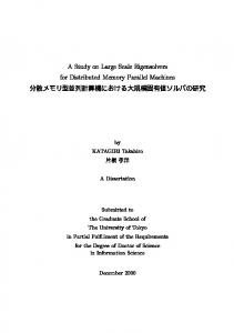
that GPU. Additionally, when the number of CPU cores exceeds the number of available GPUs, we allow for the use of software-based renderers on the extra CPUs. This code has been contributed to the VisIt project. 3.1.2. Partitioning VisIt contained a number of load decomposition strategies prior to our work. However, we found these strategies to be insufficient for a variety of reasons: • Brick-based Equalizing the distribution of work in VisIt was entirely based on bricks, or pieces of the larger data set. Our balancing algorithms use the time taken to render the previous frame to determine a weighted distribution of loads. • Master-slave Dynamic balance algorithms in VisIt are based on a master node, which tells slaves to process a brick, waits for completion, and then sends slaves a new brick to process. We implemented a flat hierarchy, as seems to be more common in recent literature [MMD06, MSE06]. • Compositing Most importantly, for our object-based decomposition to work correctly, we needed a defined ordering to perform correct compositing. The load balancing and compositing subsystems were independent prior to our work. Our system relies on a kd-tree for distributing and balancing the data. The spatial partitioning is done once initially and can be adaptively refined by the rendering times from previous frames. The initial tree only considers the number of bricks available in the data set, and attempts to evenly distribute them among processes, to the extent that is possible. When using static load balancing, this decomposition is determined and invariant for the life of the parallel job. Figure 2 depicts a possible configuration determined by the partitioner, and shows the corresponding kd-tree. When the dynamic load balancer is enabled, we use the last rendering time on each process to determine the next configuration. In our initial implementation, the metric we utilized was the total pipeline execution time to complete a frame. This included the time to read data from the disk, as well as compositing time, among other inputs. However, we found that I/O would dwarf the actual rendering time. Further, compositing time is not dependent on the distribution of bricks. This therefore proved to be a poor metric. Switching the balancer to use the total render time for all bricks on that process gave significantly better results. In order to compare different implementations, we implemented multiple load balancing algorithms, notably those described in Marchesin et al. and Müller et al.’s work [MMD06, MSE06], in order to compare different implementations. In both cases, leaf nodes represent processes, and each process has some number of bricks assigned to it. In the Marchesin-based approach, we start at the parents of

T. Fogal, H. Childs, S. Shankar, J. Krüger, R. D. Bergeron, and P. Hatcher / Visualization on Multi-GPU Clusters

Figure 2: Decomposition and corresponding kd-tree for an 8x8x3 grid of bricks divided among 4 processors. Adjacent bricks are kept together for efficient rendering and compositing. A composite order is derived dynamically from the camera location in relation to splitting planes. Note that the number of leaves in the tree is equal to the number of processes in the parallel rendering job.

the leaf nodes and work our way up the tree, searching for imbalance among siblings. If two siblings are found to be imbalanced, a single layer of bricks is moved along the splitting plane. This process continues up to the root of the tree, at which time the virtual results are committed and the new tree dictates the resulting data distribution. In the Müllerbased approach, we begin with the root node and use preorder traversal to find imbalance among siblings. Once imbalance is found, the process stops for the current frame. Instead of blindly shifting a layer of blocks between the siblings, the method derives the average rendering cost associated with a layer of bricks along the split plane, and shifts this layer if the new configuration would improve rendering times. In addition to achieving a relatively even balance among the data, the kd-tree is used in the final stages to derive a valid sort-last compositing order.

We find this architecture compelling because it removes any need to pre-process the data. VisIt’s parallel pipeline execution is based wholly around the bricks given as input to the tool. Our main restriction is the size of each individual brick: since we utilize an out-of-core volume renderer, we can stream sets of bricks through a GPU, even if the stream exceeds the maximum 3D texture size or GPU memory available. However, each individual brick must be small enough to fit within the texture memory available on a GPU. In practice, this limitation has not affected how we generated or visualized the data for this work. Should the need arise, we could re-brick the data set to sizes more amenable for visualization.

3.1.4. Compositing

Rendering is performed in parallel on all nodes. We integrated a library for both slice-based and ray-based direct volume rendering via GLSL shaders; for this work, we used the slice-based renderer. For nodes without access to a GPU, data are rendered through the Mesa library’s ‘swrast’ module, which executes vertex and fragment shaders on the CPU. Nodes render all the data they are responsible for independently, without regard for the screen space projection of the data.

After rendering completes, each node has a full image with a subset of the total data volume rendered into it. A compositing step takes these partial images and combines them to produce the final result. As noted in Section 2, we did not expect compositing to dictate the performance of our system; still, we had previously integrated the IceT parallel compositing library [MWP01], for its ease of integration and proven results. IceT gives considerably better performance than the other built-in compositors available, and so we extended the compositing code to derive a compositing order from the kdtree and hand it to IceT.

Data are forwarded “as-is” from disk, without modification or transformation to its type. In our experiments, this means that floating point data flows all the way through the pipeline, and becomes the input to the renderers – we push the native-precision data down to the GPU and render it at full resolution. Of course, data are effectively quantized due to the limited resolution of a transfer function.

IceT implements a number of different compositing modes. However, not all of them support what IceT calls ordered compositing, as is needed for object-parallel distributed volume rendering. For this work, we have utilized the so-called reduce strategy, which, since we only configure a single ‘tile’ in our system, essentially simplifies [MWP01] to an implementation of Binary Swap [MPHK94].

3.1.3. Rendering

c The Eurographics Association 2010.

T. Fogal, H. Childs, S. Shankar, J. Krüger, R. D. Bergeron, and P. Hatcher / Visualization on Multi-GPU Clusters

We implemented and tested our system on Lens, a GPUaccelerated visualization cluster housed at ORNL. However, we were only able to access 16 GPUs on that machine. In order to access a larger number of GPUs, we transitioned to Longhorn, a larger cluster housed at the Texas Advanced Computing Cluster. Specifications for each cluster are listed in Table 1. Due to machine availability and configuration, we were not able to fully utilize either machine. 4.1. Rendering Times The two dominant factors in distributed memory visualization performance are the time taken to render the data and the time taken to composite the resulting sub-images. These have the largest impact on usability, because they comprise the majority of the latency a user experiences: the time between when the user interacts with the data and when the results of that interaction are displayed.

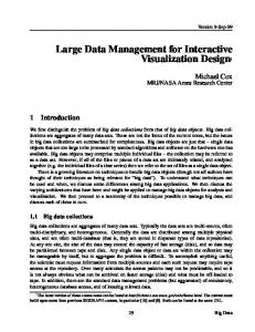
size, and number of GPUs, up to 256. Unless noted otherwise, we divided the data into a grid of 8x8x8 bricks for parallel processing (larger data sets used larger bricks), and rendered into a 1024x768 viewport. Figure 3 shows the scalability on the Longhorn cluster. The principal input which affects rendering time is the data set size, as one might expect. These runs were all done using 2 GPUs per node, except the "128 GPUs, 1 GPU/node" case, which was run on 128 nodes, each accessing a single GPU. With very large data, there is a modest increase in performance for this experimental setup. 11

3

4096 Dataset

10 9 8

Rendering Time

4. Evaluation

7 6 5 4

30

3

64 GPUs 128 GPUs 256 GPUs 128 GPUs, 1 GPU/node

2

25

Time (seconds)

1 20

256

315 342 373

512

Brick Size (voxels, cubed)

15

10

5

0 3 1024

128

3

2048

3

4096

3

8192

Dataset Size (voxels)

Figure 3: Overall rendering time when rendering to a 1024x768 viewport on Longhorn. This incorporates both rendering and compositing, and therefore shows the delay a user would experience if they used the system on a local network. Data points are the average across many frames, and error bars indicate the rendering times for the slowest and quickest frames, respectively. For these results we used a domain consisting of 133 bricks (varying brick size), with the exceptions that all runs in the 128 GPU cases used 83 bricks, and the run for the 81923 data set was done using 323 bricks. Our data originated from a simulation performed by the Center for Simulation of Accidental Fires and Explosions (C-SAFE), designed to study the instabilities in a burning helium flame. In order to study performance at varying resolutions, we resampled this data to 10243 , 20483 , 40963 , and 81923 , at a variety of brick sizes. We then performed tests, varying data resolution, image resolution, choice of brick c The Eurographics Association 2010.

Figure 4: Rendering time as a function of brick size. Error bars indicate the minimum and maximum times recorded, across all nodes, for that particular brick size; high disparity indicates the rendering time per-brick was highly variable, and load imbalance was therefore likely. All tests were done with a 40963 data set statically load balanced across 128 GPUs on 64 nodes, using a scripted camera which requested the same viewpoints each run. Note that the choice of brick size matters little in the average case, but bricks using nonpower-of-two sizes give widely varying performance. Brick sizes of 5123 technically give the best performance, though raw data show it is only hundredths of a second faster than 2563 bricks. As can be seen in Figure 4, the brick size, generally, has little impact in performance. A parallel volume renderer’s performance is dictated by the slowest component though, and therefore the average rendering time is less important than the maximum rendering time. Taking that into account, it is clear that brick sizes which are not a power of two are poor choices. Dropping down to 1283 , we can see that perbrick overhead begins to become more noticeable, impacting overall rendering times. We found larger brick sizes of 5123 get the absolute best performance, with 2563 a good choice as well, as the differences are minor enough that they may be considered sampling error. Of course, such recommendations may be specific to the GPUs used in Longhorn. We were initially surprised to find that the image resolu-

T. Fogal, H. Childs, S. Shankar, J. Krüger, R. D. Bergeron, and P. Hatcher / Visualization on Multi-GPU Clusters

Component Number of nodes GPUs per node Cores per node Graphics card Per-node Memory Processors Interconnect

Lens 32 2 16 NVIDIA 8800 GTX 64 GB 2.3 GHz Opterons DDR Infiniband

Longhorn 256 2 8 NVIDIA FX 5800 48 GB 2.53 GHz Nehalems Mellanox QDR InfiniBand

Table 1: Configuration of GPU clusters utilized.

0.48

0.44

0.42

0.4

0.38

0.36

In our initial implementation on Lens, we noticed that we began to strain the memory allocators while rendering a 30003 data set, as we approached low memory conditions. Our volume renderer automatically accounts for low memory conditions and attempts to free unused bricks before failing outright. However, an operating system will thrash excessively before finally deciding to fail an allocation, and therefore during the time leading up to a failed allocation, performance will drop considerably. Worse, we are working in a large existing code base, and attempting to manage allocations outside our own subsystem would prove unwieldy. As such, we found the original scheme to be unstable; the rendering system would create memory pressure, causing other subsystems to fail an allocation in areas where it may be difficult or impossible to ask our volume renderer to free up memory. To solve this problem, we render the data in a true outof-core fashion: bricks are given to the renderer, rendered into a framebuffer object, and immediately thrown away. We might expect that out-of-core algorithms would have more per-block overhead and therefore be slower than an in-core algorithm. As shown in Figure 5, out-of-core approach actually out-performs the analogous in-core approach even when there is sufficient memory to hold the data set. In this case, lookups were performed into a data structure with logarithmic lookup time; the in-core approach did these lookups in logarithmic time, whereas the conservative approach taken in the out-of-core algorithm meant the container maxed out at one element, which accounted for the very minor improvement to performance.

In-Core Out-of-Core

0.46

Rendering Time (seconds)

tion, while relevant, was not a significant factor in the overall rendering time. When developing single GPU applications that run on a user’s desktop, our experience was the opposite: that image size did play a significant role in performance. We at first thought this was due to skipping bricks which were ‘empty’ under our transfer function – our domain is perfectly cubic, yet as is displayed in Figure 1, very little of the domain is actually visible – but even after changing to a transfer function with no “0” values in the opacity map, rendering times changed very little. We concluded that the data sizes are so large compared to the number of pixels rendered that the image size is not relevant as a factor.

0

10

20

30

40

50

60

70

Frame

Figure 5: Rendering times, per frame, for the in-core and out-of-core approaches to rendering a 10243 data set (which fits comfortably in memory) across 16 GPUs. Additional processing in the out-of-core case does not negatively impact performance.

4.1.1. Readback and Compositing In earlier results, particularly with GPU-based rendering architectures, the community was generally concerned with the time required to read the resulting image data from the GPU and into the host’s memory [MMD08]. Our study did not provide corroboration of this concern, which we interpret as a positive data point with respect to evolving graphics subsystems. Our system did demonstrate that this time increased as the resolution grew, but as can be seen in Table 2, even at 1024x768 this step took only thousandths of a second. As expected, the time required for image composition is significantly reduced when taking advantage of the GPUs available in a visualization cluster. Since a GPU can render much faster than a software-based renderer, one can achieve acceptable rendering performance using far fewer nodes. Furthermore, because compositing scales with the number of nodes involved in the compositing process, compositing performance improves significantly when utilizing fewer nodes. c The Eurographics Association 2010.

T. Fogal, H. Childs, S. Shankar, J. Krüger, R. D. Bergeron, and P. Hatcher / Visualization on Multi-GPU Clusters

Dataset Size 10243 20483 40963 81923

Rendering (s) 0.06141 0.35107 2.50984 19.60648

Readback (s) 0.00328 0.00377 0.00377 0.00373

Compositing (s) 0.06141 0.07673 0.29533 0.51799

Total (s) 0.12610 0.43157 2.80894 20.12820

Table 2: Breakdown of the different pipeline stages for various data set sizes, when running on 256 GPUs and rendering into a 1024x768 viewport. All times are in seconds. The 10243 , 20483 , and 40963 case used 133 bricks (varying brick size); the 81923 case used 323 bricks, making each brick 2563 . Compositing time rises only artificially; if a node finishes rendering before other nodes, the time it must wait was included under ‘Compositing’ due to an artifact of our sampling code. Thus, the data imply that larger data sets see more load imbalance.

4.2. Load Balancing We also sought to examine the utility of load balancing algorithms for our system. We have implemented the algorithms as presented in two recent parallel volume rendering papers, and compared rendering times to each other and to a statically balanced case. Figure 6 illustrates the comparisons, where the times shown are the maximum on all processes. We did a variety of experiments with multiple load balancer implementations, using 8 or 16 GPUs. Our initial flythrough sequence proved to be inappropriate for the application of a load balancer, as there was not enough imbalance in the system to observe a significant benefit. We then attempted to zoom out of the dataset, but rendering times increasing on all nodes was not a case the balancers we implemented could effectively deal with: we found many cases where the balancers would shift data to a node that was previously idle or at least doing very little work, and a frame or two later the workload on such nodes would spike. This occurred because these nodes had both 1) received new data as part of the balance and, 2) retained old data as part of the initial decomposition or older balancing processes. The sudden additional workload of previously invisible bricks caused these nodes to overcompensate, sending data to other “idle” nodes – nodes which would experience the same problem a frame or two later. In previous work, authors have praised the effect load balancing has when zooming in to a data set. This naturally creates imbalance, as some nodes end up with data which are not rendered under the current camera configuration, and therefore the node has no work to do. With the implementations we recreated as faithfully as possible, we did find that zooming in to the data set was a task that was well-suited for load balancing. Still, we encountered issues even with this case. For the algorithm given in [MMD06], we observed that data would move back and forth between nodes quite frequently, having a negative impact on overall rendering time. We therefore introduced a ‘threshold’ parameter to the existing algorithm, in an attempt to limit this ‘ping-pong’ behavior. As we move up the tree, imbalance between the left and right subtrees is subject to this threshold; if it does not exceed the threshold, the imbalc The Eurographics Association 2010.

Figure 6: The maximum rendering time across all nodes under various balancing algorithms. The numbers after some algorithms indicate thresholds: rendering disparity under these thresholds is ignored.

ance is ignored. This is a very useful parameter for ensuring that we do not move data too eagerly. Generally, setting this threshold too high will yield behavior equivalent to the static case; setting it to low leads to a considerable amount of unnecessary data shifting, and we found that this in many cases overcompensated for minor, expected variations (such as those one might expect from differing brick sizes; see Figure 4). For example, see Figure 6, in which low thresholds display an obvious ‘ping-pong’ effect as nodes overcompensate for increased rendering load. Müller et al. describe a different balancing system [MSE06]. This system calculates the average cost of rendering a brick, and therefore has a clearer idea of what the effect of moving a given set of bricks will have on overall system performance. Further, they introduce additional parameters which add some hysteresis to the system, which can help reduce the ‘ping-pong’ effect of nodes sending data to a neighbor, just to receive in the next frame when the neighbor becomes overloaded. We found that this algorithm did do intelligent balancing for reasonable settings of these parameters, and the addi-

T. Fogal, H. Childs, S. Shankar, J. Krüger, R. D. Bergeron, and P. Hatcher / Visualization on Multi-GPU Clusters

by doing so the algorithm could obtain the global knowledge it needs to balance data effectively. Both of these extensions are left to future work. In Section 1, we noted a variety of questions which the design of our system allows us to answer.

Figure 7: Per-process rendering times for the ‘Müller’ line given in Figure 6.

tional parameters could be successfully used to reduce excess data reorganization. Still, we found two issues with the approach: for one, the assumption that ‘all bricks are equal’ did not pan out for our work. Even assuming uniform bricks for a data set (true for our case, but likely not in a general system), one can see in Figure 4 that the time to render a brick sees variation on the order of a second. Secondly, despite experimenting with parameter settings, we found it difficult to get the algorithm to choose the ‘best’ set of nodes for balancing. In many cases, we found a particular node was an outlier, consistently taking the most time to render per frame. Yet it was common for this algorithm to balance different nodes. While rendering times would generally improve, the system’s performance is determined by the slowest node, and therefore making the fast nodes faster does not help overall performance. This was apparent in the tests described in 6: the algorithm quite clearly balanced between some of the nodes, but the slowest node was never balanced, and therefore the uservisible performance for this run was equivalent to the static case. Figure 7 shows a more detailed analysis of the execution of the Müller algorithm that generated the data for Figure 6. The per-node rendering times in Figure 7 show that process 7 is usually the last process to finish and is often much slower than the next to the last. As evident from the lack of sudden discontinuities in that process’ rendering times, however, no bricks from process 7 move to other nodes. Therefore rendering times decrease but the maximum rendering time does not change. We theorize that additions to the algorithm to learn weights for each individual brick would yield fruitful results. Furthermore, the algorithm explicitly attempts to avoid visiting the entire tree, as an attempt to bound the maximum time needed to determine a new balancing. In our work, we did not observe cases where iterating through nodes in the tree had a measurable impact on performance, and feel that

• Rendering vs. Compositing. As shown in Table 2, subsecond rendering times are achieved using a very small number of nodes, relative to previous work. This relieves a significant source of work for compositing algorithms. • Overhead of GPU Transfer. Table 2 shows readback time to be on the order of thousandths of a second for common image sizes. Measuring texture upload rates is difficult with the asynchronous nature of current drivers and OpenGL, but we did not find evidence to suggest this was a bottleneck. • Importance of Load Balancing. A dynamic load balancer can have a very worthwhile impact on performance. However, it can also lower the performance of the system. Load balancers generally come with some number of tunable parameters, and useful settings for these parameters are difficult to determine a priori, and likely impossible for an end-user to effectively set. We observed that dynamic load balancing for volume rendering struggled in some of the cases often encountered in real world environments and, for this reason, believe there is still a gap before deploying these techniques in production systems. We see a great opportunity for future work in this area. • Viability. As displayed mostly by Figure 3 and Table 2, rendering extremely large data sizes – up to 81923 voxels – is possible on relatively few nodes. Further, data sets up to 20483 can be rendered at approximately two frames per second.

5. Conclusions With this study, we demonstrated that GPU accelerated rendering provides compelling performance for large scale data sets. Figure 3 demonstrates our system rendering data sets which are among some of the largest reported thus far, using far fewer nodes than previous work. This work shows that a multi-GPU node is a great foundational ‘building block’ to compose larger systems capable of rendering very large data. As the performance-price ratio of a GPU is higher (provided it can effectively parallelize the workload) than CPU-based solutions, this work makes the case for spending more visualization supercomputing capital on hardware acceleration, and acquiring smaller yet more performant clusters. Reports on the time taken for various pipeline stages demonstrate that PCI-E bus speeds are fast enough that readback performance is not as great of a concern as it was a few years ago. However, it remains to be seen if contention will become an issue if individual nodes are made ‘fatter’, utilizing additional GPUs. The 1 GPU per node results given in Figure 3 suggests that multiple GPUs do contend for rec The Eurographics Association 2010.

T. Fogal, H. Childs, S. Shankar, J. Krüger, R. D. Bergeron, and P. Hatcher / Visualization on Multi-GPU Clusters

sources, but at this scale the differences are not yet significant enough to warrant moving away from the more costeffective ‘fat’ node architecture. Given the relatively few nodes needed for good performance on large data, and external work scaling compositing workloads out to tens of thousands of cores, it seems likely that the relatively ‘thin’ 2-GPU-per-system architecture can be made to scale to even larger systems. 5.1. Future Work We would like to study our system with higher image resolutions, such as those available on a display wall, and larger numbers of GPUs. At some point, we expect compositing to become a significant factor in the amount of time needed to volume render large data, but we have not approached the cross-over point in this work, due to the use of ‘desktop’ image resolutions and low numbers of cores. Our system allows substituting a Mesa-based software renderer when a GPU is not available. This provided a convenient means of implementation for an existing large software system, in particular because it allows pipeline execution to proceed unmodified through the rendering and compositing stages. However, tests very quickly showed that using software renderers when a GPU was available was not worthwhile, and usually ended up hurting performance more than helping. Therefore, we traded access to more cores for the guarantee that we will obtain GPUs for each core we do get. An alternate system architecture would be to decouple the rendering process from the other work involved in visualization and analysis, such as data I/O, processing, and other pipeline execution steps. In this architecture, all nodes would read and process data, but processed, visualizable data would be forwarded to a subset of nodes for rendering and compositing. The advantage gained is the ability to tailor the available parallelism to the visualization tasks of data processing and rendering, which, as we have found, can benefit from vastly different parallel decompositions. The disadvantages are the overhead of data redistribution, and the wasted resources that arise from allowing non-GPU processes to sit idle while rendering. Our compositing algorithm assumes that the images from individual processors can be ordered in a back-to-front fashion to generate the correct image. For this paper, we met this requirement by using regular grids, which are easy to load balance in this manner. It should be possible to also handle certain types of curvilinear grids and perhaps AMR grids. Extensions to handle unstructured grids would be difficult, but represent an interesting future direction. Load balancing is an extremely difficult problem, and we have just scratched the surface here. The principal difficulty in load balancing is identifying good parameters to control how often and to what extent the balancing occurs. We c The Eurographics Association 2010.

would like to see ideas and algorithms which move in the direction of user-friendliness: determining the most relevant parameters and deriving appropriate values for them automatically.

6. Acknowledgments The authors would like to thank Gunther Weber and Mark Howison at LBNL for productive discussions, as well as Sean Ahern at ORNL for numerous discussions on ‘decoupled’ processing and rendering, which we unfortunately did not have time to consider in depth for this work. This research was made possible in part by the Office of Advanced Scientific Computing Research, Office of Science, of the U.S. Department of Energy under Contract No. DE-AC02-05CH11231 through the Scientific Discovery through Advanced Computing (SciDAC) program’s Visualization and Analytics Center for Enabling Technologies (VACET), by the NIH/NCRR Center for Integrative Biomedical Computing, P41-RR12553-10 and by Award Number R01EB007688 from the National Institute Of Biomedical Imaging And Bioengineering, by the Cluster of Excellence “Multimodal Computing and Interaction” at the Saarland University, and by the Center for the Simulation of Accidental Fires and Explosions at the University of Utah, which was funded by the U.S. Department of Energy under Contract No. B524196, with supporting funds provided by the University of Utah Research fund. Resources were utilized at the Texas Advanced Computing Center (TACC) at the University of Texas at Austin and at the National Center for Computational Sciences at Oak Ridge National Laboratory, which is supported by the Office of Science of the U.S. Department of Energy under Contract No. DE-AC0500OR22725.

References [CBB∗ 05] C HILDS H., B RUGGER E., B ONNELL K., M EREDITH J., M ILLER M., W HITLOCK B., M AX N.: A Contract Based System For Large Data Visualization. In Proceedings of IEEE Visualization 2005 (2005). http://www.idav.ucdavis.edu/ func/return_pdf?pub_id=890. [CCF94] C ABRAL B., C AM N., F ORAN J.: Accelerated volume rendering and tomographic reconstruction using texture mapping hardware. In VVS ’94: Proceedings of the 1994 symposium on Volume visualization (New York, NY, USA, 1994), ACM, pp. 91– 98. http://doi.acm.org/10.1145/197938.197972. [CDM06] C HILDS H., D UCHAINEAU M., M A K.-L.: A scalable, hybrid scheme for volume rendering massive data sets. In Proceedings of Eurographics Symposium on Parallel Graphics and Visualization (May 2006), pp. 153–162. http://www.idav. ucdavis.edu/publications/print_pub?pub_id=892. [CN94] C ULLIP T. J., N EUMANN U.: Accelerating Volume Reconstruction With 3D Texture Hardware. Tech. Rep. TR93-027, University of North Carolina at Chapel Hill, 1994. http://graphics.usc.edu/cgit/pdf/papers/ Volume_textures_93.pdf.

T. Fogal, H. Childs, S. Shankar, J. Krüger, R. D. Bergeron, and P. Hatcher / Visualization on Multi-GPU Clusters [DCH88] D REBIN R. A., C ARPENTER L., H ANRAHAN P.: Volume Rendering. In SIGGRAPH ’88: Proceedings of the 15th annual conference on Computer graphics and interactive techniques (New York, NY, USA, 1988), ACM, pp. 65–74. http: //doi.acm.org/10.1145/54852.378484. [EP07] E ILEMANN S., PAJAROLA R.: Direct Send Compositing for Parallel Sort-Last Rendering. In Proceedings of the Eurographics Symposium on Parallel Graphics and Visualization (2007), pp. 29–36. http://doi.acm.org/10.1145/1508044. 1508083. [HBC10] H OWISON M., B ETHEL E. W., C HILDS H.: MPIhybrid Parallelism for Volume Rendering on Large, Multi-core Systems. In Eurographics Symposium on Parallel Graphics and Visualization (EGPGV) (Norrköping, Sweden, May 2010). LBNL-3297E. [HHN∗ 02] H UMPHREYS G., H OUSTON M., N G R., F RANK R., A HERN S., K IRCHNER P. D., K LOSOWSKI J. T.: Chromium: A Stream-Processing Framework for Interactive Rendering on Clusters. In SIGGRAPH ’02: Proceedings of the 29th annual conference on Computer graphics and interactive techniques (New York, NY, USA, 2002), ACM Press, pp. 693– 702. http://citeseerx.ist.psu.edu/viewdoc/summary? doi=10.1.1.19.7869. [Hsu93] H SU W. M.: Segmented Ray Casting for Data Parallel Volume Rendering. In PRS ’93: Proceedings of the 1993 Symposium on Parallel Rendering (New York, NY, USA, 1993), pp. 7– 14. http://doi.acm.org/10.1145/166181.166182. [KW03] K RÜGER J., W ESTERMANN R.: Acceleration Techniques for GPU-based Volume Rendering. In Proceedings IEEE Visualization 2003 (2003). http://wwwcg.in.tum.de/ Research/data/vis03-rc.pdf. [Lev90] L EVOY M.: Efficient Ray Tracing of Volume Data. ACM Trans. Graph. 9, 3 (1990), 245–261. http://doi.acm.org/10. 1145/78964.78965. [Max95] M AX N.: Optical Models for Direct Volume Rendering. IEEE Transactions on Visualization and Computer Graphics 1, 2 (1995), 99–108. http://www.llnl.gov/graphics/docs/ OpticalModelsLong.pdf.

[MSE06] M ÜLLER C., S TRENGERT M., E RTL T.: Optimized Volume Raycasting for Graphics-Hardware-based Cluster Systems. In Eurographics Symposium on Parallel Graphics and Visualization (EGPGV06) (2006), Eurographics Association, pp. 59–66. http://www.vis.uni-stuttgart.de/ger/ research/pub/pub2006/egpgv06-mueller.pdf. [MWP01] M ORELAND K., W YLIE B. N., PAVLAKOS C. J.: Sort-Last Parallel Rendering for Viewing Extremely Large Data Sets on Tile Displays. In IEEE Symposium on Parallel and Large-Data Visualization and Graphics (2001), pp. 85– 92. https://cfwebprod.sandia.gov/cfdocs/CCIM/docs/ PVG2001.pdf. [PD84] P ORTER T., D UFF T.: Compositing Digital Images. In SIGGRAPH ’84: Proceedings of the 11th annual conference on Computer graphics and interactive techniques (New York, NY, USA, 1984), ACM, pp. 253–259. http://doi.acm.org/10. 1145/964965.808606. [PYR∗ 09] P ETERKA T., Y U H., ROSS R., M A K.-L., L ATHAM R.: End-to-End Study of Parallel Volume Rendering on the IBM Blue Gene/P. In Proceedings of the ICPP’09 Conference (September 2009). http://vis.cs.ucdavis.edu/Ultravis/ papers/129_peterka-icpp09-finalpaper.pdf. [PYRM08] P ETERKA T., Y U H., ROSS R., M A K.-L.: Parallel volume rendering on the ibm blue gene/p. In Proceedings of Eurographics Parallel Graphics and Visualization Symposium (EGPGV 2008) (April 2008), pp. 73–80. http://vis. cs.ucdavis.edu/papers/EGPGV_08.pdf. [SMW∗ 04] S TRENGERT M., M AGALLÓN M., W EISKOPF D., G UTHE S., E RTL T.: Hierarchical visualization and compression of large volume datasets using gpu clusters. In In Eurographics Symposium on Parallel Graphics and Visualization (EGPGV04) (2004 (2004), pp. 41–48. [WE98] W ESTERMANN R., E RTL T.: Efficiently Using Graphics Hardware in Volume Rendering Applications. In ACM SIGGRAPH 1998 (1998). http://doi.acm.org/10.1145/ 280814.280860.

[MCEF94] M OLNAR S., C OX M., E LLSWORTH D., F UCHS H.: A Sorting Classification of Parallel Rendering. IEEE Comput. Graph. Appl. 14, 4 (1994), 23–32. http://doi.acm.org/10. 1145/1508044.1508079. [MMD06] M ARCHESIN S., M ONGENET C., D ISCHLER J.-M.: Dynamic Load Balancing for Parallel Volume Rendering. In 6th Eurographics Symposium on Parallel Graphics and Visualization (May 2006), pp. 43–50. http://people.freedesktop.org/ ~marcheu/egpgv06-loadbalancing.pdf. [MMD08] M ARCHESIN S., M ONGENET C., D ISCHLER J.-M.: Multi-GPU Sort-Last Volume Visualization. In EG Symposium on Parallel Graphics and Visualization (EGPGV’08), Eurographics (April 2008). http://icps.u-strasbg.fr/ ~marchesin/egpgv08-multigpu.pdf. [MPHK93] M A K. L., PAINTER J. S., H ANSEN C. D., K ROGH M. F.: A Data Distributed, Parallel Algorithm for Ray-Traced Volume Rendering. In PRS ’93: Proceedings of the 1993 symposium on Parallel Rendering (New York, NY, USA, 1993), ACM, pp. 15–22. http://doi.acm.org/10.1145/166181.166183. [MPHK94] M A K.-L., PAINTER J. S., H ANSEN C. D., K ROGH M. F.: Parallel Volume Rendering Using Binary-Swap Compositing. IEEE Comput. Graph. Appl. 14, 4 (1994), 59– http://citeseerx.ist.psu.edu/viewdoc/summary? 68. doi=10.1.1.104.3283. c The Eurographics Association 2010.