Jun 18, 2014 - diffusion process exits from a domain containing its endpoints, as the ... the estimates for the probability of exit from a domain that are our final.
arXiv:1406.4649v1 [math.PR] 18 Jun 2014
Large Deviation asymptotics for the exit from a domain of the bridge of a general Diffusion Paolo Baldi, Lucia Caramellino, Maurizia Rossi Dipartimento di Matematica, Universit`a di Roma Tor Vergata, Italy Abstract We provide Large Deviation estimates for the bridge of a d-dimensional general diffusion process as the conditioning time tends to 0 and apply these results to the evaluation of the asymptotics of its exit time probabilities. We are motivated by applications to numerical simulation, especially in connection with stochastic volatility models.
AMS 2000 subject classification: 60F10, 60J60 Key words and phrases: Large Deviations, conditioned Diffusions, exit times, stochastic volatility.
1
Introduction
In this paper we give Large Deviation (LD) estimates for the probability that a d-dimensional pinned diffusion process exits from a domain containing its endpoints, as the conditioning time goes to 0. This investigation is motivated by applications to numerical simulation in presence of a boundary, as explained in [4] and [6], where a correction technique is developed requiring at each iteration of the Euler scheme to check whether the conditioned diffusion touches the boundary. In the most common case, where the exit from a domain is actually the crossing of a barrier, people have resorted so far to the approximation of the conditioned diffusion with the one that has its coefficients frozen at one of the endpoints, so that the computation is reduced to exit probabilities for the Brownian bridge that are well known, also for curved boundaries (see [17] and [4]). In [11] this technique is well developed producing also error estimates. In recent years however the application to stochastic volatility models of the freezing approximation has prompted to further the investigation in order to obtain precise estimates and also to check the amount of error produced by the method of freezing. As remarked in [4] the exact computation of this probability is, in general, very difficult and it is suggested that as the time step in simulation is in general very small, one could be sufficiently happy with the equivalent of this probability as the conditioning time goes to 0. The natural tool are therefore LD’s or, better, sharp LD’s, as developed in [4] and [6]. Our first step is a pathwise Large Deviation Principle (LDP) for the bridge of a general diffusion whose proof turns out to be particularly simple. Our results are in some sense weaker than the existing literature, but apply to a general class of diffusions. See in particular [3], [13] and [14]. As already mentioned this LD result is not a complete LDP for the conditioned diffusion but it is sufficient in order to derive the estimates for the probability of exit from a domain that are our final goal. 1
Considering applications to stochastic volatility models we must mention that some of them do not fall into the domain of application of our result. It is the case for instance of the Heston model. In the last section, on the other hand, we show how to apply our estimates to the Hull and White model. In §1 we introduce notations and recall known results needed in the sequel. In §2, using the well known equivalence between LDP and Laplace Principle we prove a Large Deviation estimate for a large class of conditioned diffusion processes. These LD estimates are sufficient in order to derive in §4 LD estimate for the probability of the conditioned diffusion to exit a given, possibly unbounded, open set D. The main tool in this section is an extension of Varadhan’s lemma to possibly discontinuous functionals. In §5 we give an application to the Hull-White stochastic volatility model, pointing out in particular that the method of freezing the coefficients can lead to significantly wrong appreciations. The computations turn out to be particularly simple in this case as the model is then closely related to the geometry of the hyperbolic half-plane H.
2
Notations
In this paper ξ denotes a d-dimensional diffusion process satisfying the Stochastic Differential Equation (SDE) on an open set S ⊂ Rm dξs = b(ξs ) ds + σ(ξs ) dBs , ξ0 = x
(2.1)
for some locally Lipschitz coefficients b : S → Rd and σ : S → Rd×m , B being a m-dimensional Brownian motion. We assume that ξ has a transition density, denoted by p from now on. Assumption 1 We assume that the SDE (2.1) has a.s. infinite lifetime, i.e. that inf{t, ξt 6∈ S} = +∞. For t > 0 we denote ξ t the rescaled process, i.e. ξst = ξst for s ∈ [0, 1]; it is immediate that ξ t satisfies the SDE √ dξst = tb(ξst ) ds + t σ(ξst ) dBs , (2.2) ξ0t = x , for a possibly different Brownian motion B. For y ∈ S, the pinned process conditioned by ξt = y is the time inhomogeneous Markov process ξb = ξbx,y whose transition density is, for 0 ≤ u ≤ v ≤ t and z 1 , z 2 ∈ Rd , p(v − u, z1 , z2 )p(t − v, z2 , y) · (2.3) pb(u, v, z1 , z2 ) = p(t − u, z1 , y) t Let now ξbt = ξbx,y be the rescaled pinned process given by
whose transition function is of course
ξbst = ξbts ,
pbt (u, v, z1 , z2 ) =
s ∈ [0, 1] ,
p(t(v − u), z1 , z2 )p(t(1 − v), z2 , y) · p(t(1 − u), z1 , y)
(2.4)
(2.5)
Let us denote Cx ([0, 1], Rd ) (or for brevity Cx ) the space of continuous functions γ : [0, 1] → Rd with starting point γ0 = x. We denote Xs the canonical application Xs : Cx → Rd defined as Xs (γ) = γ(s) and by (Fs )s the canonical filtration Fs = σ(Xu , u ≤ s).
2
We shall denote Ptx the law on Cx of the rescaled process ξ t and Etx the corresponding expectation b tx,y the law of ξbt . We have and similarly we shall denote P b tx,y dP p(t(1 − s), Xs , y) = , dPtx |F p(t, x, y)
0≤s 0 and (ξbut )0≤u≤1 the rescaled process ξbut = ξbut . Then, for every 0 ≤ s < 1, ξbt , as a (Cx , Fs )-valued random variable, satisfies a LDP with respect to the rate function ( I(γ) − I(γ0 ) if γ1 = y b I(γ) = (3.2) +∞ otherwise
and inverse speed function g(t) = t, where γ0 is the geodetic for the metric (2.7) connecting x to y, i.e. b lim sup t log P(ξbt ∈ A1 ) ≤ − inf I(γ) γ,γ∈A1
t→0
bt
b lim inf t log P(ξ ∈ A2 ) ≥ − inf I(γ) t→0
γ,γ∈A2
for every closed set A1 ⊂ Cx and every open set A2 ⊂ Cx .
Remark that Theorem 3.2 does not give a LDP on the whole of F1 , but that the rate function (3.2) does not depend on s. Proof. It is well-known that the LDP is equivalent to the Laplace principle (see [9], Theorem 1.2.3 e.g.), i.e. we must prove that for every bounded continuous Fs -measurable functional F : Cx → R, � � b b t e− 1t F = − inf (F (γ) + I(γ)) . (3.3) lim t log E x,y t→0
γ∈Cx
F being Fs -measurable, we have by (2.6)
4
� � � � b tx,y e− 1t F = − log p(t, x, y) + log Etx e− 1t F p(t(1 − s), Xs , y) . log E − 12
(3.4)
2
Varadhan’s estimate (2.9) immediately gives limt→0 t log p(t, x, y) = d(x, y) = −I(γ0 ). Let us turn our attention to the remaining term � 1 � � � 1 log Etx e− t F p(t(1 − s), Xs , y) = log Etx e− t (F −t log p(t(1−s),Xs ,y)) .
We shall now take advantage of the LD estimate enjoyed by the family of probabilities (Ptx )t . If we 1 were allowed to replace in the r.h.s. the quantity t log p(t(1 − s), Xs , y) by − 2(1−s) d(Xs , y)2 , which is its limit as t → 0 by (2.9), we could apply Varadhan’s Lemma 2.1 and the LDP that holds for the unconditioned processes (Ptx )t and find that � 1 � 1 � 2 � 1 lim t log Etx e− t (F −t log p(t(1−s),Xs ,y)) = lim t log Etx e− t (F + 2(1−s) d(Xs ,y) ) = t→0 t→0 � � (3.5) 1 d(γs , y)2 . = − inf F (γ) + I(γ) + γ∈Cx 2(1 − s) In Lemma 4.4 we prove that � inf F (γ) + I(γ) + γ∈Cx
� 1 γ ) + I(b γ )) d(γs , y)2 = inf (F (b γ b,b γ1 =y 2(1 − s)
so that (3.5) will allow to end the proof. Let us prove (3.5) rigorously. Let � � 1 ks := inf F (γ) + I(γ) + d(γs , y)2 . γ∈Cx 2(1 − s)
Let, for ε > 0 fixed, R be large enough so that � F (γ) + I(γ) + inf γ,γs ∈BR (x)
� 1 d(γs , y)2 ≤ ks + ε , 2(1 − s)
where BR (x) stands for the open ball for the distance d centered at x with radius R. Remark that, thanks to Assumption 2, BR (x) ⊂ S. By Varadhan’s estimate (2.9), BR (x) being compact, we have that for t small and uniformly for z ∈ BR (x), −ε −
1 1 d(z, y)2 ≤ t log p(t(1 − s), z, y)) ≤ ε − d(z, y)2 , 2(1 − s) 2(1 − s)
so that, by the LD lower bound enjoyed by (Ptx )t , � 1 � lim inf t log Etx e− t (F −t log p(t(1−s),Xs ,y)) ≥ t→0 � 1 � ≥ lim inf t log Etx e− t (F −t log p(t(1−s),Xs ,y)) 1{Xs ∈BR (x)} ≥ t→0 � 1 � 2 1 ≥ lim inf t log Etx e− t (F +ε+ 2(1−s) d(Xs ,y) ) 1{Xs ∈BR (x)} ≥ t→0 � � 1 d(γs , y)2 − ε ≥ F (γ) + I(γ) + ≥− inf 2(1 − s) γ,γs ∈BR (x) � � 1 ≥ − inf F (γ) + I(γ) − d(γs , y)2 − 2ε . γ 2(1 − s) � � 1 Let us look for a converse inequality and decompose the quantity Etx e− t (F −t log p(t(1−s),Xs ,y) into the sum of the two terms � 1 � I1 (t) = Etx e− t (F −t log p(t(1−s),Xs ,y)) 1{Xs ∈BR (x)} , � � 1 (3.6) I2 (t) = Etx e− t (F −t log p(t(1−s),Xs ,y)) 1{Xs ∈BR (x) c } . 5
By Varadhan’s lemma 2.1, the set {γs ∈ BR (x)} being closed, we have similarly
� 1 � I1 (t) = lim sup t log Etx e− t (F −t log p(t(1−s),Xs ,y)) 1{Xs ∈BR (x)} ≤ t→0
� 1 � 2 1 ≤ lim sup t log Etx e− t (F −ε+ 2(1−s) d(Xs ,y) ) 1{Xs ∈BR (x)} ≤ t→0
≤−
inf
γ,γs ∈BR (x)
� F (γ) + I(γ) +
� 1 d(γs , y)2 + ε ≤ −ks + 2ε . 2(1 − s)
As for I2 (t), let R0 > 0 be large enough so that y ∈ BR0 (x) and let C = supu≤1,z∈∂BR0 (x) p(u, z, y). As the density p is a continuous function of (t, x) as far as z is away from y, we have C < +∞. as a function of (t, x) By a simple application of the strong Markov property (see Proposition 3.4 below), we have for R > R0 p(u, z, y) ≤ C for every 0 ≤ u ≤ 1, z ∈ BR (x)c . Taking R > R0 , we have, denoting by M a bound for |F |,
� 1 � 1 � � I2 (t) ≤ Etx e− t (F −t log p(t(1−s),Xs ,y)) 1{Xs ∈BR (x)c } ≤ C Etx e− t F 1{Xs ∈BR (x)c } ≤ M
≤ C e t Ptx (Xs ∈ BR (x)c ) .
By the LDP satisfied by Xs under Ptx as t → 0, we have for t small 1 lim sup t log Ptx (Xs ∈ BR (x)c ) ≤ − R2 , 2 t→0 recall actually that, as BR (x) is the ball in the distance d, we have I(γ) ≥ 21 R2 for every path γ such that γs ∈ BR (x)c . Thanks to Assumption 2 we can choose R as large as we want. In particular we can have R > M + ks . With this choice of R we have � 1 � lim sup t log Etx e− t (F −t log p(t(1−s),Xs ,y)) 1{Xs ∈BRc } ≤ M − R < −ks . t→0
Finally, putting together the estimates we have � 1 � lim sup Etx e− t (F −t log p(t(1−s),Xs ,y)) = max(−ks , M − R) = −ks t→0
which finishes the proof.
� Remark, as a consequence of Theorem 3.2, that the rate function Ib of the rescaled bridge does not depend on the drift b of (2.1). Lemma 3.3 For every continuous Fs -measurable functional F we have � � � 1 γ ) + F (b γ) . inf I(γ) + F (γ) + 2(1−s) d(γs , y)2 = inf I(b γ
γ ,b b γ1 =y
Proof. The main point is the rather obvious inequality: Z 1 1 d(γ1 , γs )2 ≤ ha(γu )−1 γ˙ u , γ˙ u i du 1−s s
which becomes an equality if γ in the time interval [s, 1] is the geodesic connecting γs to γ1 .
6
(3.7)
(3.8)
Let γ b be such that I(b γ ) < +∞ and b γ1 = y and let γ be the path that coincides with b γ until time s and is constant in [s, 1]. We have F (b γ ) = F (γ), as the two paths γ and γ b coincide up to time s and also, of course, Z s Z 1 ha(b γu )−1 γ b˙ u , γ b˙ u i du = ha(γu )−1 γ˙ u , γ˙ u i du . 0
0
Therefore, thanks to (3.8), I(b γ) = ≥
1 2
Z
0
1
1 2
Z
0
s
1 ha(b γu )−1 γ b˙ u , γ b˙ u i du + 2
ha(γu )−1 γ˙ u , γ˙ u i du +
Z
s
1
ha(b γu )−1 γ b˙ u , γ b˙ u i du ≥
1 1 d(γs , y)2 = I(γ) + d(γs , y)2 . 2(1 − s) 2(1 − s)
As F (γ) = F (b γ ), we have proved that, for every γ b such that γ b1 = y, there exists an unconstrained path γ such that 1 F (γ) + I(γ) + 2(1−s) d(γs , y)2 ≤ F (γ) + I(b γ) . (3.9) Conversely, for a given path γ such that I(γ) < +∞, let b γ the path that coincides with γ up to time s and then connects γ bs = γs with the value γ b1 = y with a geodesic in the time interval [s, 1]. For such a path γ b we have equality in (3.8) and therefore Z Z 1 1 1 s ha(b γu )−1 γ b˙ u , γ b˙ u i du + ha(b γu )−1 γ b˙ u , γ b˙ u i du = I(b γ) = 2 0 2 s Z 1 s 1 = d(γs , y)2 ≤ ha(γu )−1 γ˙ u , γ˙ u i du + 2 0 2(1 − s) Z 1 1 1 ≤ d(γs , y)2 = ha(γu )−1 γ˙ u , γ˙ u i du + 2 0 2(1 − s) 1 = I(γ) + d(γs , y)2 . 2(1 − s) Therefore, again using the fact that F (γ) = F (b γ ), we see that in (3.9) also the ≥ sign holds, so that the equality is established. � The following result, that was used in the proof of Theorem 3.2, is a simple consequence of the strong Markov property. Proposition 3.4 Let X be a S-valued continuous Markov process with transition density p enjoying the Feller property. Let D ⊂ S an open set and y ∈ D. Then if z ∈ Dc we have p(t, z, y) = Ez [1{ρ 0. Thanks to Theorem 3.2 we have � � b b tx,y τ < s ≥ − inf b tx,y τ < s = lim t log P I(γ) . (4.2) lim t log P D t→0
t→0
γ,τD (γ) 0. Let us denote by G the set of continuity points γ of F such that I(γ) < +∞ and τ (γ) ≤ 1. For every γ ∈ G, let δ = δ(γ) be such that if kζ − γk∞ < δ, then |F (ζ) − F (γ)| < ε and I(ζ) ≥ I(γ) − ε. Let us denote Sγ,δ the open ball centered at γ and with radius δ in the uniform topology. Let us fix ρ > 0. By hypothesis the family (Sγ,δ(γ) )γ∈G is an open cover of {I ≤ ρ} ∩ {τ ≤ 1} which is a compact set. Let (Sγi ,δ(γi ) )i=1,...,m a finite subcover. Then m � � X Etx e−F/t 1{τ ≤1} ≤ i=1
where Γ = {I > ρ} ∩ {τ ≤ 1} \ Z t log
S
i
Sγi ,δ(γi )
Z
Sγi ,δ(γi )
e−F/t 1{τ ≤1} dPtx +
Z
Γ
e−F/t dPtx
Sγi ,δ(γi ) . Therefore for i = 1, . . . m � � e−F/t dPtx ≤ t log e−(F (γi )−ε)/t Ptx (Sγi ,δ(γi ) )
so that there exists t0 > 0 such that, for t ≤ t0 , Z t log e−F/t dPtx ≤ −F (γi ) + ε − I(γi ) + 2ε Sγi ,δ(γi )
and such that t log
Z
Γ
� e−F/t dPtx ≤ t log eM/t Ptx (Γ) ≤ M − ρ + ε .
Therefore, for t ≤ t0 , � � � t log Etx e−F/t 1{τ ≤1} ≤ max −F (γi ) − I(γi ) + 3ε, i = 1, . . . , m, M − ρ = � = − min F (γi ) + I(γi ) − 3ε, i = 1, . . . , m, −M + ρ and ρ, ε being arbitrary, we find (4.8).
� Remark 4.8 In [3] it is proved a LD estimate for the bridge of a hypoelliptic diffusion process. It is however required that the process takes its values on a compact manifold. Remark that Theorem 3.2 remains true under this weaker assumption, just replacing the Riemannian distance with the associated sub-Riemannian distance (see [3] e.g. for details) and Varadhan’s estimate (2.9) with its hypoelliptic counterpart ([16], [15]). As for the estimates of exit from a domain the main missing 11
link is Lemma 4.6: it is not obvious that given a point x ∈ ∂D there exists a path of finite energy for which the exit time from D and the one from D coincide. Recall that a point x ∈ ∂D is said to be characteristic if the subspace linearly generated by the random fields in the diffusion coefficient at x is tangent to ∂D. We have that Lemma 4.6, and therefore the upper bound, still holds in the hypoelliptic case if the boundary ∂D does not have characteristic points and under this additional assumption also the argument concerning the lower bound remains valid. We choose not to address this issue as the applications that are the object of our interest are not in this direction.
5
Application: the Hull-White stochastic volatility model
As mentioned in §1, the interest of estimates of the kind of Proposition 4.5 concerns mainly the application to simulation. Let us consider the following model � p v2 � dξt = b − t dt + vt ρ dB1 (t) + vt 1 − ρ2 dB2 (t) 2 dvt = µvt dt + σvt dB1 (t) ,
(5.1)
where −1 ≤ ρ ≤ 1, σ > 0 and B = (B1 , B2 ) is a 2-dimensional Brownian motion. This is actually the Hull and White’s model of stochastic volatility. Remark that the process (ξ, v) takes its values in R × R+ . We first investigate the simpler model with ρ = 0 and σ = 1, i.e. � � v2 dξt = b − 2t dt + vt dB1 (t) (5.2) dvt = µvt dt + vt dB2 (t) . The corresponding metric tensor is a
−1
(ξ, v) =
�
1 v2
0
0 1 v2
�
(5.3)
and we recognize the metric structure of the Poincar´e half-space H. Recall that H = R × R+ with the Riemannian distance (see [1] e.g. or wikipedia) � (x2 − x1 )2 + (y2 − y1 )2 � , d((x1 , y1 ), (x2 , y2 )) = acosh 1 + 2y1 y2
(5.4)
lim d((x1 , y1 ), (x2 , y)) = +∞ ,
(5.5)
whereas the geodesics are pieces of circles whose center lies on the y = 0 axis. Remark that distances become very large near the axis y = 0, actually y→0
so that the boundary is at an infinite distance from every point of H. It is easy to conclude that Assumption 2 is satisfied and that Proposition 4.5 holds in this situation. Figure 1 shows the path minimizing the functional for the conditioned diffusion with endpoints (1, .2) and (2, .5) in comparison with the one that would be given by the method of freezing the coefficients (as the metric tensor is always a multiple of the identity, the minimizer does not depend on the point at which the coefficients are frozen, whereas the value of the rate function does). It appears that the two behaviors are quite different. Not surprisingly also the values of the rate function produced by the two models are very different: freezing the coefficients at (2, .5) would give the value 6.0, against the value with the true model 3.8 whereas freezing at (1, .2) or at some point 12
.5 .25
.. .. .. . . . . . . . . . . . . . . . . . . . . . . . . . . . . . . . .. . . . . . . . . ............... ........... . . . . . . . . . . . . . . . . ......... .. ...... . . . . . . . . . . . . ....• ...... . . . . . . . . .. (2.5,0.97) . . .... ..... .. ...... ..... ...... ...... ... ..... ..... . . . . . . .. . . . .... .... .. ... .... . . . . .. . . .. ... . . .. . . .. .. . . .. . . .. .. . . .. . . .. .. . . .. . . ... ... ... .. . . • .... ....... ....... .. . ....... ...... (2,.5) .. . (2.5,0.43) ..... ....... • . . . ... . . . . . . .... ....... .. .. ....... ....... .. ....... ....... ... ..... ....... . . . . . . . . .... . . ....... ... •........ ....... .. (1,.2) .. .. .. .
1
2
2.5
Figure 1: Graph of the true minimizer (solid) in comparison with the one provided by the approximation with the frozen coefficients (dashes). The dotted line denotes the barrier. Here ordinates are volatility whereas the logarithm of the price are in the abscissas. between would give an even larger result. Of course this discrepancy would be more large, the more the coordinate y of the volatility approaches 0. Therefore freezing the coefficients would give for the probability pt of touching the barrier the equivalent as t → 0 (in the logarithmic sense) pt ≈ e−6/t much different from the true equivalent pt ≈ e−3.8/t . Of course this discrepancy between the true equivalent and the one produced by the method of freezing will be important when the volatility is low and perhaps acceptable when it is high. In Figure 2 we considered endpoints nearer to the barrier, a situation more realistic during a simulation. The true value of the rate function turns out to be equal to 0.119, whereas the coefficients frozen at (2.48, .12) give the approximation 0.083. the discrepancy between the two values, assuming 1 would give for the probability of exit the values a time step t = 20 ≈ e−.119·20 = 0.092
and
≈ e−.083·20 = 0.19
which is certainly not satisfactory. In this case freezing at the midpoint would give a good approximation (0.090) but, as indicated by the situation of Figure 1, this is not a general rule. ... .. .. .. .. . . . ..... ......... ... .. ...... . ..... ........ (2.5,0.108) .. .....• . .... . ...... ........ • ...... ..... ...... .. (2.5,0.104) . . . . . ... ..... ....... ..... .. .... ... .. ..... .... .. ... ...... . . .. . . .. . . ... ...... .. . . .. .... . .. . . ... ... .. . . .. (2.47,.8) ............. .. . . . .. •.... .. .. .. .. .
•................... .. .. (2.48,.12) . ..........................
.1
.07 2.45
2.5
Figure 2: Same as in Figure 1 but with values closer to the barrier. Here we computed numerically the the point at which the path that minimizes the rate function reaches the boundary.
13
Let us go back to the general model (5.1): the corresponding metric tensor is � 2 � 1 σ −σρ −1 e a (ξ, v) = 2 2 . 1 v σ (1 − ρ2 ) −σρ
Denoting, for simplicity, ρ =
p 1 − ρ2 , the linear transformation H → H �1 ρ � − σρ A= ρ 1 0 σ
(5.6)
(5.7)
turns the Riemannian metric (5.6) on H into the Poincar´e metric. It is then immediate that the Riemannian distance de associated to (5.6) is e 1 , y1 ), (x2 , y2 )) = d((ρx1 + ρy1 , y1 ), (ρx2 + ρy2 , y2 )) , d((x
(5.8)
where d is defined as in (5.4). The geodesic for d corresponding to a piece of the circle centered e i.e. a piece of the ellipse satisfying the in (α, 0) with radius R is changed into the geodesic for d, equation (ρx + ρy − α)2 + σ 2 y 2 = R2 . In practice in order to compute the equivalent of touching a barrier x = x0 for the general Hull-White model (5.1) for the diffusion conditioned between the endpoints z1 = (x1 , y1 ) and z2 = (x2 , y2 ) the simplest way is to switch to the consideration of the simpler model (5.2) conditioning between the endpoints z1′ = Az1 and z2′ = Az2 and to compute, as indicated above, the equivalent of touching the straight line x + ρρ y = ρ1 x0 ,which is the image of x = x0 through A. In this way it is possible to take advantage of the well known properties and computations of the hyperbolic half plane H.
References [1] M. Abate, Iteration theory of holomorphic maps on taut manifolds, Research and Lecture Notes in Mathematics. Complex Analysis and Geometry, Mediterranean Press, Rende, 1989. [2] R. Azencott, Grandes d´eviations et applications, Eighth Saint Flour Probability Summer School—1978 (Saint Flour, 1978), Lecture Notes in Math., vol. 774, Springer, Berlin, 1980, pp. 1–176. [3] I. Bailleul, Large deviation principle for bridges of degenerate diffusions, arXiv:1303.2854v1 (2013).
preprint
[4] P. Baldi, Exact asymptotics for the probability of exit from a domain and applications to simulation, Ann. Probab. 23 (1995), no. 4, 1644–1670. [5] P. Baldi and L. Caramellino, Asymptotics of hitting probabilities for general one-dimensional pinned diffusions, Ann. Appl. Probab. 12 (2002), no. 3, 1071–1095. [6] P. Baldi, L. Caramellino, and M. G. Iovino, Pricing general barrier options: a numerical approach using sharp large deviations, Math. Finance 9 (1999), no. 4, 293–322. [7] P. Baldi and M. Chaleyat-Maurel, An extension of Ventsel′ -Freidlin estimates, Stochastic analysis and related topics (Silivri, 1986), Lecture Notes in Math., vol. 1316, Springer, Berlin, 1988, pp. 305–327.
14
[8] P. Baldi and B. Pacchiarotti, Explicit computation of second-order moments of importance sampling estimators for fractional Brownian motion, Bernoulli 12 (2006), no. 4, 663–688. [9] P. Dupuis and R. S. Ellis, A weak convergence approach to the theory of large deviations, Wiley Series in Probability and Statistics: Probability and Statistics, John Wiley & Sons, Inc., New York, 1997. [10] I.M. Freidlin and A.D. Ventsel, Random perturbations of dynamical systems, Springer, Berlin, Heidelberg, New York, 1983. [11] E. Gobet, Weak approximation of killed diffusion using Euler schemes, Stochastic Process. Appl. 87 (2000), no. 2, 167–197. [12] A. Gulisashvili and P. Laurence, The Heston Riemannian distance function, J. Math. Pures Appl. (9) 101 (2014), no. 3, 303–329. [13] P. Hsu, Brownian bridges on Riemannian manifolds, Probab. Theory Related Fields 84 (1990), no. 1, 103–118. [14] Y. Inahama, Large deviation principle of Freidlin-Wentzell type for pinned diffusion processes, Preprint arXiv:1203.5177v3 (2012). [15] R. L´eandre, Majoration en temps petit de la densit´e d’une diffusion d´eg´en´er´ee, Probab. Theory Related Fields 74 (1987), no. 2, 289–294. [16]
, Minoration en temps petit de la densit´e d’une diffusion d´eg´en´er´ee, J. Funct. Anal. 74 (1987), no. 2, 399–414.
[17] H. R. Lerche and D. Siegmund, Approximate exit probabilities for a Brownian bridge on a short time interval, and applications, Adv. in Appl. Probab. 21 (1989), no. 1, 1–19. [18] S. R. S. Varadhan, On the behavior of the fundamental solution of the heat equation with variable coefficients, Comm. Pure Appl. Math. 20 (1967), 431–455.
15