Aug 1, 2013 - ... operator describing the particle exchange has a discrete spectrum. Under this condition,. arXiv:1308.0082v1 [cond-mat.stat-mech] 1 Aug ...
Large deviation function and fluctuation theorem for classical particle transport Upendra Harbola Inorganic and Physical Chemistry, Indian Institute of Science, Bangalore
Christian Van den Broeck Hasselt University, B-3500 Hasselt, Belgium
arXiv:1308.0082v1 [cond-mat.stat-mech] 1 Aug 2013
Katja Lindenberg Department of Chemistry and Biochemistry and BioCircuits Institute, University of California San Diego, La Jolla, CA 92093-0340 We analytically evaluate the large deviation function in a simple model of classical particle transfer between two reservoirs. We illustrate how the asymptotic large time regime is reached starting from a special propagating initial condition. We show that the steady state fluctuation theorem holds provided that the distribution of the particle number decays faster than an exponential, implying analyticity of the generating function and a discrete spectrum for its evolution operator.
I.
INTRODUCTION
The second law of thermodynamics has two major ingredients: the existence, in an equilibrium state, of a state function called the entropy, and the increase of the total entropy in a spontaneous transition between two equilibrium states. The discovery of the fluctuation theorem entails a double departure from this standard formulation of the second law. Entropy is defined in nonequilibrium states, and it is even defined for a single realization in a non-extensive system, where it is a stochastic quantity which can increase as well as decrease with time. Furthermore, the fluctuation theorem states (in its simplest formulation) that the fluctuating total entropy production ∆Stot obeys a symmetry property: P (∆Stot )/P (−∆Stot ) = exp ∆Stot /kB [1]. This equality implies the second law inequality h∆S tot i ≥ 0. The fluctuation theorem was first discovered in an “asymptotic version,” preceding the definition of a proper stochastic entropy [2]. In this version, one only focuses on the entropy production in idealized reservoirs. For a heat reservoir i at temperature T (i) , the entropy change is given by ∆S (i) = Q(i) /T (i) , where Q(i) is the net amount of heat transferred from the system to reservoir i. Note that Q(i) and hence ∆S (i) = Q(i) /T (i) are well defined even though the system need not be at equilibrium. Furthermore, in the case of a small system, the amount of heat Q(i) will differ from one realization to another, so that this is a genuine stochastic quantity. Coming back to the fluctuation theorem, one notes that the total entropy Pchange is the sum of all the contributions: ∆Stot = i ∆S (i) + ∆S, which includes the entropy change ∆S of the system. Since the entropy productions in the reservoirs are easier to monitor than the nonequilibrium stochastic system entropy ∆S (where, for simplicity, we also avoid a discussion of the possible contribution to the entropy coming from interaction terms between system and reservoirs), it is of interest to identify situations in which the latter contribution is negligible. A good candidate is the asymptotic time regime
for systems operating under steady state nonequilibrium conditions. Indeed one intuitively expects that the heat (and/or particle) flows will be proportional to time, while the (stochastic) entropy of the system, being in a steady state, should remain more or less constant. Hence the latter contribution becomes negligible in the long-time limit. This was indeed proven to be the case for a class of systems with bounded energy. One can then write P P (i) P ( i ∆S (i) ) /kB i ∆S P ∼ e , P (− i ∆S (i) ) known as the steady-state fluctuation theorem [3]. This asymptotic version of the fluctuation theorem can, however, break down when the energy of the system is unbounded [4]. A well documented example is that of Brownian particle in contact with one or several heat reservoirs [5–9]. The large deviation function probes exponentially unlikely events for the heat evacuated to the reservoirs. Such an event can however be the result of an exponentially unlikely initial energy of the system. In this case the entropy contribution of the system is no longer negligible and a fluctuation theorem in terms of reservoir entropies alone breaks down. Here, we study the less-documented case of particle transport. More precisely, we analyze particle transport through a system in contact with particle reservoirs [10]. We evaluate analytically the large deviation function for the particle flux. We find that the asymptotic fluctuation theorem is satisfied under “natural” conditions, which are typical for the distribution of the number of particles. More precisely, whereas the Boltzmann factor allows for large energies, albeit in an exponentially unlikely way, the distribution P (n) for having n particles in a system typically decays faster than exponential, due to the indistinguishability property giving rise to a n! contribution in the denominator. As a result the generating function F (s) = Σn sn P (n) is analytic in s in the entire complex plane, and the stochastic operator describing the particle exchange has a discrete spectrum. Under this condition,
2 we are able to prove the validity of the steady state fluctuation theorem. When the system is coupled to particle reservoirs, a cumulated particle flux develops between the system and the reservoirs. The probability distribution of this flux typically depends on time in a complicated way. One may wonder whether there exist special initial conditions for which the functional form of this distribution does not change with time. We will identify such an initial distribution for the model under consideration. Note that, from the point of view of a detector (observer), the natural initial condition is to start to count the particle flux at time zero starting from a zero value. However, as we shall see, this is an unnatural initial condition from the “system’s point of view,” as correlations then develop between the observed flux and the state of the system. The paper is organized as follows. In the next section we present the particle transfer model and its basic mathematical framework. In Sec. III we introduce the generating function method to compute statistics of the particle fluxes between system and reservoirs. In Sec. IV we identify the joint distribution of system state and particle fluxes that propagates in time. In the long-time limit, it approaches an asymptotic regime characterized by a large deviation function. In Sec. V we verify the steady-state fluctuation relation and discuss its validity in the specific context of particle transfer.
II.
MASTER EQUATION
We consider a system which can exchange matter (particles) with two particle baths, with chemical potentials µ(1) and µ(2) and temperatures T (1) and T (2) , respectively. The number of particles in the system will be denoted by n, n ∈ N. For simplicity, we will operate in the limit of non-interacting, classical but indistinguishable particles, each of energy �. We furthermore assume that the exchange of particles between system and baths can be described by a Markovian jump process. Consider an instant at which the system contains n particles. (i) Let k+ be the rate for a particle to jump into the sys(i) tem, while nk− is the rate for a particle to jump out of the system, to and from thermal bath i, with i = 1, 2. The corresponding master equation for the probability to have n-particles in the system at time t then reads ∂ P (n; t) = k+ P (n − 1; t) + (n + 1)k− P (n + 1; t) ∂t − (k+ + nk− )P (n; t), (1) with k± =
(1) k±
+
(2) k± .
(2)
We start with a number of remarks. First, when in contact with a single bath i, the steady state probability solution of (1) reduces to the Poissonian equilibrium
(i)
distribution Peq (n), (i) Peq (n) =
ρni −ρi e , n!
(3)
with a corresponding average number of particles ρi given by (i)
ρi =
k+
(i)
.
(4)
k−
We mention for further use the relation between this equilibrium density and the reservoir properties (β (i) = 1/kB T (i) ), ρi = ge−β
(i)
(�−µ(i) )
,
(5)
where g is the number of single particle states with energy � in the system and µi is the chemical potential of the i-th bath. Since we are dealing with the classical limit, g should be much larger than n and the exponential in (5) is much smaller than unity. Equation (5) is the detailed balance condition for the transport between the system and the i-th reservoir. Second, due to the combinatorial factor n!, the proba(i) bility distribution Peq (n) decays more quickly than exponentially for large n. Since there is a compelling physical reason for this factor, namely, the indistinguishability of particles, we expect this to be a genuine feature of a particle distribution function, and we will assume below a faster than exponential decay for the probability distribution even when operating under nonequilibrium conditions. Third, we mention the following exact time-dependent solution of (1), namely, a propagating Poisson distribution: P (n; t) =
(ρ(t))n e−ρ(t) n!
(6)
with the mean number of particles in the system at time t given by � � k+ k+ ρ(t) = + ρ(0) − e−k− t . (7) k− k− At steady state, ρss = k+ /k− . Hence, the particle distribution maintains a Poissonian equilibrium-like shape, even though it is in a nonequilibrium state. We next turn to our main quest, namely, the study of the fluctuation theorem. We first identify the entropy (i) change ∆Sr in bath (i), for a given total elapsed time t: Q(i) T (i) (� − µ(i) )Ni =− T (i) ρi = kB Ni ln g
∆S (i) =
(8)
3 Here Ni is a register that adds (subtracts) 1 whenever a particles crosses from heat bath i to the system (from the system to heat bath i). Thus, Ni is the net number crossing from bath i to the system between time 0 and t plus the number that was on the register at time t = 0 (see below). All the particles have the same energy �. In going from the first to the second line, we have used the conservation of energy, with the change in bath energy −�Ni being equal to heat plus chemical energy, Q(i) − µ(i) Ni . Transition to the third line is based on (5). The evaluation of the stochastic bath entropies is thus reduced to that of the number of particles Ni (Ni ∈ Z, i = 1, 2) transferred from baths to the system in time t. Since these numbers are deterministic functions of the system dynamics, the enlarged set of variables n, N1 , N2 again defines a Markov jump process, and the joint probability P (n, N1 , N2 ; t), to find n particles in the system while having a cumulative transfer of N1 , N2 particles in time t, evolves according to the following master equation: ∂ (1) P (n, N1 , N2 ; t) = k+ P (n − 1, N1 − 1, N2 ; t) ∂t (2) + k+ P (n − 1, N1 , N2 − 1; t) (1)
+ (n + 1)k− P (n + 1, N1 + 1, N2 ; t) (2)
+ (n + 1)k− P (n + 1, N1 , N2 + 1; t) − (k+ + nk− )P (n, N1 , N2 ; t). (9)
The parameters λ = {λ1 , λ2 } are so-called “counting parameters” that keepi track of the net number of particles transferred between the system and the corresponding reservoirs. We shall use λ to denote a dependence on λ1 and λ2 . By combination with (9) we find ∂ Fλ (s; t) = Lλ (s)Fλ (s, 0), ∂t
(12)
where the operator L is defined as, Lλ (s) = k− αλ s + k− βλ
∂ ∂ − k− s − k+ ∂s ∂s
(13)
with (1)
(2)
αλ =
k+ eλ1 + k+ eλ2 , k−
βλ =
k− e−λ1 + k− e−λ2 . k−
(1)
(14)
(2)
(15)
Since the dependence on the counting parameters in Eq. (12) is parametric, it suffices to evaluate the eigenvectors and eigenvalues of L as an operator with respect to the variable s. Let Ψλ (s) be an eigenvector of Lλ (s) with eigenvalue ζλ , Lλ (s)Ψλ (s) = ζλ Ψλ (s).
(16)
As we proceed to show, it is possible to find an exact time-propagating solution of this equation, which allows us to find the asymptotic large time properties, in particular those of the stochastic entropy. This solution furthermore illustrates how this asymptotic regime is reached in the course of time. We finally note that due to particle conservation, the following identity holds at all times:
With the expression (13) for the operator, the eigenfunctions are found by straightforward integration,
n(t) = N1 (t) − N1 (0) + N2 (t) − N2 (0) + n(0), (10)
We now make the following crucial assumption, already mentioned in the introduction: We request that the eigenfunctions be analytic in the variable s in the entire complex plane. Analyticity imposes two restrictions on the exponent gλ : it must be greater than or equal to zero, gλ ≥ 0 and it must be an integer. Hence, setting gλ = l with l ∈ N we find from (18) for the eigenspectrum of the operator Lλ
where n(0), N1 (0) and N2 (0) are, respectively, the number of particles in the system and the number of particles on registers 1 and 2 at time t = 0. We make two observations whose significance will reveal themselves when discussing the time-propagating solution of (9). First, while it is quite natural and tempting, from the observer’s point of view, to choose N1 (0) = N2 (0) = 0, the choice of N1 (0) and N2 (0) is in principle free, and could even be stochastic. Second, it follows from (10) that the condition n(0) = N1 (0) + N2 (0) propagates in time, i.e., it implies that n(t) = N1 (t) + N2 (t) holds at all times.
Ψλ (s) = (s − βλ )
gλ = αλ βλ −
(l)
The solution of the master equation is facilitated by switching to the following generating function: ∞ ∞ X X Fλ (s; t) = eλ1 N1 +λ2 N2 sn P (n, N1 , N2 ; t). N1 ,N2 =−∞ n=0
(11)
k+ + ζλ . k−
ζλ = k− αλ βλ − k+ − lk− ,
(17)
(18)
l ∈ N.
(19)
The corresponding eigenfunction can now be written in the following compact way: Ψλ (s) =
GENERATING FUNCTION
exp {αλ (s − βλ )} ,
where
(l)
III.
gλ
∂l exp {αλ (s − βλ )} . l ∂αλ
(20)
At this point, we make two observations. First, the eigen(l) value ζλ depends on λ only via λ = λ1 − λ2 and is invariant under the following interchanges: ρ1 λ ↔ −λ − ln (21) ρ2 λi ↔ −λi − ln(ρi ) for i = 1 and 2. (22)
4 The eigenfunctions themselves, however, do not obey this symmetry. This property will be crucial to verify the steady state fluctuation theorem. Second, the above set of eigenfunctions is complete in the sense that any analytic function of s can be expanded in terms of this basis. Furthermore, the expansion is unique as it corresponds to a Taylor expansion around the point βλ . Hence we obtain the following explicit expression for the generating function (assumed to be analytic in s) obeying (12): Fλ (s; t) =
∞ X
(l)
(l)
(l)
aλ Ψλ (s) etζλ ,
Poissonian distributions. One can verify that the “natuK ral initial condition” P (N1 , N2 ; t = 0) = δN δ K does 1 ,0 N2 ,0 not lead to a time propagating solution, that is, it cannot (0) be expressed solely in terms of the eigenvector Ψλ (s). This could have been anticipated from the fact that the propagating condition n(0) = N1 (0) + N2 (0) would then imply n(0) = 0, which is incompatible with the ”propagating” steady state statistics P st (n) for n.
(23)
l=0 (l)
where aλ is expansion coefficient of the eigenfunction (l) Ψλ (s) for the initial function Fλ (s, 0). In the sequel, we will focus on a particular simple initial condition, corre(l) K (0) sponding to aλ = δl,0 aλ , where δ K is the Kronecker delta. One reason is obvious: the corresponding eigenfunction is dominating the long-time limit, since it has the lowest eigenvalue, cf. (19). The other reason is that such an initial condition corresponds, for an appropri(0) ate choice of the coefficient aλ , to a genuine probability (0) distribution. The explicit expression for Ψλ (s) suggests (0) the following choice for aλ : (0)
aλ = eαλ βλ −k+ /k− ,
(24)
where the subtraction of k+ /k− guarantees normalization. Referring to the appendix for the calculation of the inverse, we find that it leads to the following initial probability distribution: k ! ! − + (1) N1 (2) N2 k+ k+ e k− P (n, N1 , N2 ; t = 0) = N1 !N2 ! k− k− K × δn,N Θ(N1 )Θ(N2 ), 1 +N2
(25)
where Θ(x) is a Heaviside theta-function. The Kronecker delta in (25) imposes the condition that initially n(0) = N1 (0) + N2 (0). This condition was to be expected since, as mentioned earlier, it propagates in time with n = N1 + N2 at all times. The corresponding reduced distribution for the number of particles in the system, P st (n), is, as expected, the steady state distribution, cf. (6), ρ e P (n) ≡ P (n; t = 0) = , n!
IV.
PROPAGATING SOLUTION AND LARGE DEVIATION FUNCTION
Our main focus is the evaluation of the joint reduced distribution, P (N1 , N2 ; t). Its generating function Fλ (t) is found by setting s = 1 in (23): Fλ (t) =
n −ρ
st
FIG. 1. (Color online) Upper panel: Initial distribution P (N1 , N2 ; t = 0), cf. Eq. (31), and its projection onto the (1) (1) (2) (N1 , N2 ) plane. Parameters are: k+ = 2.0, k− = 0.2, k+ = (2) 0.1 and k− = 1.0. Lower panel: Initial probability distribu(2) (1) (1) tion correspondng to equilibrium values k+ = k− = k+ = (2) k− = 1.
(26)
with ρ = k+ /k− . The reduced distribution for the initial cumulated particle transfer P (N1 , N2 ; t = 0), see also Fig. 1, is obtained by summation of (25) over n. The summation only affects the Kronecker delta; hence P (N1 , N2 ; t = 0) is obtained from Eq. (25) by the reK placement of the Kronecker delta δn,N with Θ(N1 + 1 +N2 N2 ), but this factor is superfluous due to the presence of Θ(N1 )Θ(N2 ). We conclude that the reduced initial distribution P (N1 , N2 ; t = 0) is a product of two independent
=
∞ X
eλ1 N1 +λ2 N2 P (N1 , N2 ; t)
N1 ,N2 =−∞ ∞ X (l) (l) aλ Ψλ (s l=0
(l)
= 1) etζλ .
(27)
(28)
The l = 0 term dominates the series in Eq. (23) for asymptotically long times t → ∞. Alternatively, this term corresponds to the full solution at all times for the initial condition identified in the previous section. We henceforth consider this case and can thus write (0)
(0)
(0)
Fλ (t) = aλ etζλ Ψλ (s = 1),
(29)
5 (0)
with aλ given by Eq. (24). The corresponding joint probability P (N1 , N2 ; t) is computed by taking the inverse transform of (29): I I dλ2 −(λ1 N1 +λ2 N2 −tζ (0) ) dλ1 λ e P (N1 , N2 ; t) = 2πi 2πi (0)
(0)
× aλ Ψλ (s = 1).
(30)
Switching to the integration variable λ = λ1 − λ2 , and expanding the exponential of αλ /k− which appears inside (0) Ψλ (s = 1), cf. Eq. (20), Eq. (30) can be rewritten as I ∞ X dλ1 λ1 (m−N1 −N2 )) 1 1 e P (N1 , N2 ; t) = m m! k 2πi − m=0 I (0) dλ (1) (2) × (k+ + k+ e−λ )m eλ(N2 +tζλ ) e−k+ /k− . (31) 2πi (0)
Since ζλ and αλ βλ are functions of only λ, the integral K over λ1 reduces to the Kronecker delta δm,N . Ex1 +N2 panding the exponential in αλ βλ , the remaining integral over λ can be performed. Following the same steps which led to (25), we obtain the following propagating solution for the joint distribution function: P (N1 , N2 ; t) = ×
×
e
−t
(1) (2) (2) (1) k k +k k + − + − k−
e−k+ /k− (N1 + N2 )! !N2 ! (1) N1 k+ x (2) k− 2k−
NX 1 +N2
�
m=0
N1 + N2 m
�
(2) (2)
k+ k−
!m/2
(1) (1) k+ k−
× Im−N2 (xt) Θ(N1 + N2 ),
(32)
2 x= k−
(33)
FIG. 2. (Color online) Probability distribution function, P (N1 , N2 ; t), for different times, t = 1, 10 and 100 (top to bottom). As time increases, the distribution becomes more peaked around the second diagonal, illustrating the convergence of j1 = N1 /t to −j2 = −N2 /t.
where q
(1) (2) (1) (2)
k+ k+ k− k−
and In (y) is the modified bessel function of the first kind of order n. It is straightforward to check that for t = 0 this reduces to the product of Poissonians, cf. (25). The distribution function (32) is shown in Fig. 2 for different values of t. We next focus on the large t limit. Since the particle fluxes N1 and N2 diverge for t → ∞, we introduce the fluxes per unit time ji = Ni /t. In this limit, an additional simplification takes place as one finds asymptotically that the stochastic quantities j1 and j2 become identical (see Fig. 2). Hence, the statistics in the long time limit are expressed in terms of a single flux j1 = −j2 = j. The corresponding probability distribution function for j has the typical shape from large deviation theory, namely, P (j; t) ∼ e
−tL(j)
with the large deviation function 1 L(j) = − lim ln P (j; t) t→∞ t
(34)
(35)
given by the following convex non-negative function: (2) (1) (1) (2) p k+ k− + k+ k− − x2 + j 2 k− ! p ρ2 x2 + j 2 + j j p . + ln 2 ρ1 x2 + j 2 − j
L(j) =
(36)
From Eq. (32), the probability P (N, t) to have N1 = −N2 = N at time t takes a simple form, −t
P (N ; t) = e
k
(1) (2) (2) (1) k +k k + − + − k−
(1) (2)
k+ k−
!N/2
(2) (1)
k+ k− × e−k+ /k− IN (xt) .
(37)
In Fig. 3 we plot −(1/t) ln P (N, t) to illustrate how the asymptotic form of the large deviation function is approached in the course of time. The dots represent the exact analytical result, Eq. (36). An alternative procedure to obtain the large deviation function is to work via the scaled cumulant generating
6
FIG. 3. (Color online) The function − ln P (N ; t)/t, and its limiting form, the large deviation function (35), L(j), as a function of time t = 10, 20, 40, 200 (solid curves,top to bottom). j = N/t is plotted along the x-axis. The parameter values are the same as in Fig. 1. The dots represent the analytical result in Eq. (36) and the dotted curve is a guide to the eye. The dashed curve with a minimum at j = 0 represents the (1) (1) (2) (2) equilibrium case (ρ1 = ρ2 ) for k+ = k− = k+ = k− = 1. The dotted vertical line represents the average hji, Eq. (44).
FIG. 4. The cumulant generating function Gλ for the same parameter values as in Fig. 1. Note the symmetry around λ = (1/2) ln(ρ2 /ρ1 ) (dotted line), in agreement with the fluctuation theorem, cf. Eq. (51) .
Furthermore, all odd and even cumulants of j are proportional to the first and second cumulants, respectively:
function,
κ2 (j) , tn−2 κ1 (j) κn (j) = n−1 , t
1 ln Fλ (t). (38) t For large t, the generating function Fλ (t) in Eq. (29) can be approximated by
κn (j) =
Gλ =
t
Fλ (t) = e
(1) (2) k k + − k−
(eλ −1)+t
k
(2) (1) k + − k−
(e−λ −1)
,
(39)
which on substituting in (38) gives (1) (2)
(2) (1)
k k k k Gλ = + − (eλ − 1) + + − (e−λ − 1). k− k−
(40)
Gλ is related to L(j) by a Legendre transformation, L(j) = extλ (λj − Gλ ) .
(41)
The extremum is found at 1 λ(j) = ln 2
! p ρ2 j 2 + x2 + j p . ρ1 j 2 + x2 − j
(42)
Substituting this result in (41), we recover Eq. (36). The cumulant generating function Gλ allows for a swift calculation of the cumulants of the current. For large times, the nth cumulant κn (N1 ) of N1 , the net number of particles transferred between the system and the reservoir by time t, is obtained from Gλ as dn Gλ κn (N1 ) = t . (43) dλn λ=0
Thus according to (43), all cumulants κn (N1 ) vary linearly with time. For particle current j, the average and the variance are given by: � 1 � (1) (2) (2) (1) κ1 (j) = k+ k− − k+ k− , (44) k− � 1 � (1) (2) (2) (1) κ2 (j) = k+ k− + k+ k− . (45) tk−
V.
n even n odd.
(46)
FLUCTUATION THEOREM
From (8), we find that the total entropy production in the reservoirs (divided by kB ) is asymptotically given by Σi ∆S (i) ρi = Σi Ni ln kB g ρ1 ∼ tj ln , ρ2
(47) (48)
where we used the fact that asymptotically j = j1 = −j2 (Ni = tji ). The steady state fluctuation theorem then requires that ρ1 P (j) ∼ etj ln ρ2 , P (−j)
(49)
or, more precisely, that the large deviation function, Eq. (36), obeys the symmetry relation, L(j) − L(−j) = j ln(ρ2 /ρ1 ),
(50)
which is easily verified by Eq. (36). This symmetry of the large deviation function implies an analogous symmetry for the cumulant generating function, Gλ = G−λ−ln(ρ1 /ρ2 ) .
(51)
We recall that the analyticity of the generating function for the particle number n is an essential assumption in the above derivation of the steady state fluctuation
7 theorem. This requires that the corresponding probability P (n) decay faster than an exponential in n. This property is verified by the steady state Poisson distribution, Eq. (6), which decays (for large n) logarithmically faster than the exponential: P (n) ∼ e−n ln(n) , for n � 1. It is therefore quite natural to assume that the initial condition satisfies the same property, that is, that it ask decays faster than an exponential. Without this assumption, exponentially rare fluctuations in the initial particle distribution will lead to a breakdown of the fluctuation theorem. We finally mention that the large deviation function Eq. (36) is identical to that for a random walker on a line (1) (2) (2) (1) with jump rates k+ k− /k− to the right and k+ k− /k− to the left. The physical interpretation is clear. Since the probability distribution of the number of particles contained in the system decays faster than an exponential, the large deviation statistics is essentially described by the transfer statistics between the reservoirs only, cf. the asymptotic identity of j1 and −j2 . It is intuitively clear that this long-time process will be identical to the asymptotic properties of a random walk. An identical result is obtained for the effusion of particles between two reservoirs connected through a small opening [11].
ACKNOWLEDGMENTS
UH acknowledges financial support from the Indian Institute of Science, Bangalore, India. CVdB thanks the European Science Foundation through the network “Exploring the Physics of Small Devices.” KL gratefully acknowledges support of the Office of Naval Research through Grant No. N00014-13-1-0205. .....
(0)
Substituting for Ψλ (s) from Eq. (20), we get I I dλ1 −λ1 N1 ds 1 P (n, N1 , N2 ; t = 0) = e n+1 2πi s 2πi I dλ2 −λ2 N2 sαλ −k+ /k− (53) e e e 2πi Next we expand the exponential which contains the variable s. This allows us to perform the s-integral and gives K the Kronecker delta function δn,m . We find I I 1 dλ1 −λ1 N1 dλ1 n P (n, N1 , N2 ; t = 0) = e α n! 2πi 2πi λ e−λ2 N2 e−k+ /k− .
(54)
n Using αλ from (14), and expanding αλ using binomial expansion, we obtain k
P (n, N1 , N2 ; t = 0) =
e
(1)
k+ k−
−
n! I
×
− k+
!n
n � � X n l=0
dλ1 λ1 (n−l−N1 ) e 2πi
I
l
(2)
k+
!l
(1)
k+
dλ1 λ2 (l−N2 ) e . 2πi (55)
The integrals over λ1 and λ2 give Kronecker deltas, K K δn,N and δl,N , respectively. Using these in (55), 1 +N2 2 we get (for n = N1 + N2 ) Eq. (25). An alternative method to obtain the probability distribution is to expand the generating function Fλ and compare it term-by-term with the definition (11). Here we present this method to recover Eq. (25). At t = 0, the generating function Fλ is (keeping only the l = 0 term) (0)
(0)
Fλ (s; 0) = aλ Ψλ (s). (0)
(56)
(0)
Substituting for aλ and Ψλ (s), we can re-express it as APPENDIX DERIVATION OF EQ. (25)
In order to compute the initial probability distribution for which only the term with l = 0 in the series (23) (0) (0) survives, we need to inverse transform aλ Ψλ (s), where (0) we choose aλ = eαλ βλ −k+ /k− . Note that for λ = 0, (0) aλ = 1 to preserve the normalization of the probability distribution. This is not the only possible choice for (0) aλ , however this choice leads to a simple natural initial Poissoinian distribution, cf. Eq. (25), which propagates in time. Thus we have, I P (n, N1 , N2 ; t = 0) =
I ds n−1 dλ1 −λ1 N1 s e 2πi 2πi I dλ2 −λ2 N2 (0) (0) e aλ Ψλ (s). (52) 2πi
k
− k+ sαλ −
e ∞ k X sn n − + = e k− α n! λ n=0
Fλ (s; 0) = e
! ∞ (1) n X sn k+ =e n! k− n=0 ! � � n (2) m X n k+ × e(n−m)λ1 emλ2 . (57) (1) m k+ m=0 k
− k+
−
Since m, n are dummy variables, we can rewrite the last line as ! ∞ X n (1) n k n X k+ s − k+ Fλ (s; 0) = e − n! k− n=0 N2 =0 ! � � (2) N2 k+ n e(n−N2 )λ1 eN2 λ2 . (58) × (1) N2 k+
8 In order to put it in a convenient form which will allow an easy comparison with (11), we introduce a Kronecker K delta δn−N . This allows us to rewrite Eq. (58) as, 2 ,N1 ! ∞ X n ∞ (1) n k n X X k+ s − k+ Fλ (s; 0) = e − n! k− n=0 N2 =0 N1 =−∞ ! � � (2) N2 k+ n K × eN1 λ1 eN2 λ2 δN .(59) 1 ,n−N2 (1) N2 k+ Finally, rearranging the Kronecker delta and using the fact that due to the binomial coefficients all terms for
[1] G. N. Bochkov and Y. E. Kuzovlev, Physica A 106, 443 (1981); ibid 480 (1981); D. Evans, E. G. D. Cohen and G. P. Morris, Phys. Rev. Lett. 71, 2401 (1993); D. J. Evans and D. J. Searles, Phys. Rev. E 50, 1645 (1994); G. Gallavotti and E. G. D. Cohen, Phys. Rev. Lett. 74, 2694 (1995); J. Stat. Phys. 80, 931 (1995); C. Jarzynski, Phys. Rev. Lett. 78, 2690 (1997); Phys. Rev. E 56, 5018 (1997); G. E. Crooks, J. Stat. Phys. 90, 1481 1(998); L. Lebowitz and H. Spohn, J. Stat. Phys. 95, 333 (1999); T. Hatano and S. I. Sasa, Phys. Rev. Lett. 86, 3463 (2001); T. Speck and U. Seifert, Europhys. Lett. 74, 391 (2006). R. J. Harris and G. M. Schutz, J. Stat. Mech. P07020 (2007); M. Esposito and C. Van den Broeck, Phys. Rev. Lett.104, 090601 (2010); M. Esposito, U. Harbola, and S. Mukamel, Phys. Rev. E 76, 031132 (2007). [2] U. Seifert, Phys. Rev. Lett. 95, 040602 (2005).
N2 < 0 and n < N2 vanish, we can recast this expression as k
Fλ (s; 0) = e
− k+
−
∞ X
∞ X
∞ X
sn eλ1 N1 eλ2 N2
n=0 N2 =−∞ N1 =−∞
1 × N1 !N2 !
(1)
k+ k−
!n
(2)
k+
(1) k+
!N2 K δn,N .(60) 1 +N2
Comparing this with (11), we recover (25). Similar steps can be followed to obtain the time dependent joint distribution function given in Eq. (32).
[3] M. Esposito, U. Harbola and S. Mukamel, Rev. Mod. Phys. 81, 1665 (2009). [4] J. Farago, J. Stat. Phys. 107 781 (2002); ibid, Physica 331, 69 (2003). [5] R. van Zon and E. G. D. Cohen, Phys. Rev. Lett. 91, 110601 (2003). [6] P. Visco, J. Stat. Mech. P06006 (2006). [7] M. Baiesi, T. Jacobs, C. Maes, and N. S. Skantzos Phys. Rev. E 74, 021111 (2006). [8] A. Puglisi, P. Visco, E. Trizac and F. van Wijland, Phys. Rev. E 73, 021301 (2006). [9] H. C. Fogedby, A. Imparato, J. Stat. Mech., P05015 (2011). [10] C. Van den Broeck and K. Lindenberg, Phys. Rev. E 86, 041144 (2012). [11] B. Cleuren, C. Van den Broeck and R. Kawai, Phys. Rev. E 74, 021117 (2006).