Large Deviations for a Point Process of Bounded Variability

Markov Processes Relat. Fields 12, 235–256 (2006)

 Markov MP Processes &R F  and Related Fields c Polymat, Moscow 2006

Large Deviations for a Point Process of Bounded Variability S. Goldstein 1 , J.L. Lebowitz 1,2 and E.R. Speer 1 1 2

Department of Mathematics, Rutgers University, New Brunswick, NJ, and IHES, Bures-sur-Yvette, France Department of Physics, Rutgers University

Abstract. We consider a one-dimensional translation invariant point process of density one with uniformly bounded variance of the number NI of particles in any interval I. Despite this suppression of fluctuations we obtain a large deviation principle with rate function F(ρ) ' −L−1 log Prob(ρ) for observing a macroscopic density profile ρ(x), x ∈ [0, 1], corresponding to the coarse-grained and rescaled density of the points of the original process in an interval of length L in the limit L → ∞. F(ρ) is not convex and is discontinuous at ρ ≡ 1, the typical profile. Keywords: large deviations, hyperuniform point processes, controlled variability AMS Subject Classification: 60G52, 60F10

1. Introduction One dimensional point processes of bounded variability (or controlled variability) are translation invariant probability measures describing systems of particles in R for which the variance of the particle number NI in an interval I is uniformly bounded: for some constant C < ∞ which is independent of I, Var(NI ) ≤ C.

(1.1)

In this paper we describe a particular class of such processes, which we call G processes and which are a special case of the self-correcting processes introduced by Isham and Westcott [1]. We compute some elementary properties of these systems and then show that they satisfy a large deviation principle. Point processes satisfying (1.1) have been studied in the statistics literature; see [1–4]. They were also investigated in [5]; the analysis in that paper and

236

S. Goldstein, J.L. Lebowitz and E.R. Speer

in the references given there was motivated by, and presented in terms of, the statistical mechanics of infinite particle systems. The main result of [5] is that the measure µ on the space of locally finite subsets of R for a process satisfying (1.1) with density ρ¯ is a superposition of mutually singular translates of some periodic measure µ0 with period ρ¯−1 : −1

µ = ρ¯

ρ¯ Z

dx µx .

(1.2)

0

Here µx is the translate of µ0 by x; the measures µx are called the periodic components of µ. (The actual condition required in [5] is tightness of the family of all random variables NI − ρ¯|I|, which is weaker than (1.1).) The constant C of (1.1) must satisfy C ≥ 1/4; in fact, if E(NI ) = k + θ with k an integer and 0 ≤ θ < 1 then, Var(NI ) = h(NI − k)2 i − θ2 = θ(1 − θ) + E (NI − k)(NI − k − 1) ≥ θ(1 − θ),

(1.3)


where the last inequality follows from the fact that NI is an integer (see [6]). The lower bound (1.3) is obtained by taking µ0 to be the point mass on a lattice with period ρ¯−1 . In general, however, µ0 need not be so rigid; it can have arbitrarily large fluctuations in particle number as long as these have small probability. One such example, the (a, b) process discussed by Lewis and Govier [2], is obtained by displacing the point ai in the lattice aZ of period ρ¯−1 = a by a random amount bi , where the variables bi are independent and have a common continuous distribution with finite first moment; see also [4]. This periodic process has bounded variances in the sense of (1.1); denoting by µ0 the measure describing it one may thus construct a (translation invariant) process of bounded variability as a superposition of translates µx of µ0 by x ∈ [0, 1), as in (1.2). These translates can be shown to be mutually singular, so that the construction provides an explicit decomposition of the process into its periodic components. There are alternate constructions for which the periodicity is not built in a priori. An example of such a point process given in [5] is that corresponding to the equilibrium state for positive point charges in a uniform negative background, usually referred to as the one-dimensional one-component plasma or Jellium. This system has very long range interactions between the particles, with the pair potential growing like |xi − xj |. The self-correcting processes of [1] are other examples; the particular class of these which is the main focus of this paper will be described in Section 2, and a brief description of the general class is given in Remark 3.1. One may of course also consider point processes satisfying conditions similar to but less restrictive than (1.1), or satisfying analogues of these conditions in

Large deviations for a point process

237

higher dimensions. We define superhomogeneous processes [7] to be translation invariant point processes in d-dimensions (on either Rd or Zd ) for which the variance of the number NB of particles in a ball B grows more slowly than the volume |B| of B, i.e., for which lim |B|−1 Var(NB ) = 0.

(1.4)

|B|→∞

It was shown by Beck [8] that Var(NB ) cannot grow more slowly (in the Cesaro mean sense) than the surface area |∂B| of B; it is thus only in one dimension that one can have translation invariant point processes with bounded variance in a ball, as in (1.1). Hyperuniform systems [9] are then defined as ones which realize this bound: Var(NB ) ≤ C|∂B|. (1.5) Thus, hyperuniform systems in one dimension are the controlled variability processes defined earlier. Examples of hyperuniform systems in dimensions d > 1 are the analogues of the (a, b) process, analyzed in [4], and the one-component plasma with log |xi − xj | interactions in d = 2 and |xi − xj |−(d−2) interactions in d > 2 [10, 11]. A well known example of a superhomogeneous but not hyperuniform process in d = 1 is the Dyson gas with logarithmic interactions, whose measure µ is (after some normalization) the same as the distribution of the eigenvalues of a random Gaussian Hermitian matrix [12]. For this system Var(NI ) ∼ log |I|. For other examples see [5, 13]. Given their definition, it is reasonable to expect that superhomogeneous systems will have a tendency to suppress also large deviations in NB . This is in fact true for most of the examples discussed above but, as we shall see, there are exceptions, at least in one dimension. We will discuss this question primarily in the context of large deviations of NI in one-dimensional systems. To obtain more information about the probability of large fluctuations in NI for |I| large we may ask, for example, for what increasing functions φ(u), u > 0, it is true that Prob(|NI − E(NI )| ≥ φ(|I|)) → 0

as |I| → ∞.

(1.6)

For processes for which the NI satisfy a standard central limit theorem — for example, the Poisson process — (1.6) holds only if φ(u) grows faster than u1/2 . For a process of bounded variability, on the other hand, it follows immediately from (1.1) that (1.6) holds whenever φ(u) → ∞ as u → ∞. When (1.6) does hold, we may ask for the rate of decay of the probability in (1.6) as |I| increases. Of particular interest is the case φ(u) = κu, for which

238

S. Goldstein, J.L. Lebowitz and E.R. Speer

we will study the probability of deviations of specific sign; with L = |I| we write 
 Prob NI − E(NI ) ≥ κL , if κ > 0, (1.7) pL (κ) ≡ 1, if κ = 0, 
 Prob NI − E(NI ) ≤ κL , if − ρ¯ ≤ κ < 0.

The random variables NI satisfy a large deviation principle with rate function ψ(κ) if pL (κ) decays as pL (κ) ' exp[−Lψ(κ)]. Many processes — again, the Poisson case is typical — do satisfy such a principle, with ψ(κ) ∼ cκ2 for κ small. What then of processes of bounded variability? (i) For the (a, b) processes, − log pL (κ) grows faster than L, so that ψ(κ) does not exist. For example, in order to have NI = 0 (corresponding to κ = −¯ ρ), each of the L/3 points in the central third of I must be displaced at least L/3 units, so that Prob(NI = 0) ≤ [Prob(bi ≥ L/3)]L/3 . (1.8) More generally, a fluctuation of size κL in NI can occur only if at least order L particles are displaced a distance at least of order L; an estimate as in (1.8), supplemented with some simple counting of the ways these displacements can occur, then verifies the result. (ii) For the one-component plasma it is believed that pL (κ) ' exp[−c(κ)L3 ], so that again ψ(κ) does not exist (although of course c(κ) is a rate function on a different scale). In d dimensions the corresponding quantity pR (κ) describing large fluctuations in NB , with B a ball of radius R, satisfies pR (κ) ' exp[−c(κ)Rd+2 ] (see [14] for the heuristic derivation of the result in 2 and 3 dimensions). We expect similar behavior for most superhomogeneous processes, for example with pL (κ) ' exp[−c(κ)L2 ] for the Dyson gas in d = 1 (see [12] for a discussion of the case κ = −¯ ρ, i.e., NI = 0). (iii) For the G process, on the other hand, we will establish in Section 4 that there does exist a rate function ψ(κ), with ψ(κ) ∼ c|κ| when κ → 0. This is a consequence of the more general large deviation theorem given in Section 3. We believe that certain other self-correcting process also satisfy a large deviation principle, as we discuss in Remark 3.1. 2. Construction and simple properties of the G process

In this section we construct the G processes with density 1; these are parameterized by a real number α > 1 (the construction for arbitrary density ρ¯ is similar, and the parameter satisfies α > ρ¯). As a first step we define a real-valued Markov process Yλ (t), for t ≥ 0, satisfying Yλ (t) > −1; here λ is a probability measure on (−1, ∞). Yλ (t) is defined by two conditions: Yλ (0) is distributed according to λ, and Yλ (t) increases at rate 1 as t increases, except at the points of a Poisson process of density α on R+ , at which it jumps down by

Large deviations for a point process

239

one unit — unless this jump would violate the condition Yλ > −1, in which case no jump occurs. It is easy to verify explicitly (see below) that this process has a unique stationary single-time distribution λ = λ0 . The corresponding translation invariant process (obtained for example by imposing the initial condition λ0 at time τ and then taking the Cesaro limit as τ → −∞) we denote by Y (t). Having defined Y , we take the points of the G process to be those points at which Y jumps; in other words, the G process is the distribution of the jump points of the Y process. We remark that the points of the G process may be viewed as the output of a so-called D/M/1 queue [15]. Let NI denote the number of points of the G process in the interval I, and write Prob for the probability measure of the Y process (e.g., on path space) and E for expectation with respect to this measure. Then clearly N(s,t] = t − s − (Y (t) − Y (s)),

(2.1)

Var(N(s,t] ) = E[((Y (t) − Y (s))2 ].

(2.2)

and Since from (2.3) below Y (t) has finite mean and variance, (2.1) and (2.2) imply that the process has density 1 and is of bounded variability. In the remainder of this section we compute some simple properties of this process, including the asymptotic value of Var(N(s,t] ) for t − s large. We first note that if λ is a probability distribution with density fλ (y) then the density fλ (y, t) for Yλ (t) satisfies fλ (y, 0) = fλ (y) and ( ∂fλ αfλ (y + 1, t) − αfλ (y, t), if y > 0, ∂fλ (y, t) + (y, t) = ∂t ∂y αfλ (y + 1, t), if y ≤ 0. The stationary probability density for Y is then seen to be ( 1 − β 1+y , if − 1 < y < 0, f (y) = (1 − β)β y , if y ≥ 0,

(2.3)

where β is the unique root of the equation β = e−α(1−β)

(2.4)

lying in the interval 0 < β < 1. From (2.3), 1 1 − , | log β| 2 1 1 2 . E(Y 2 (t)) = − + 3 | log β| log2 β E(Y (t)) =

(2.5) (2.6)

To obtain the decomposition (ref1.2) of the process into its periodic components we introduce the random variable U = Y (n) − bY (n)c, n ∈ Z, where for

240

S. Goldstein, J.L. Lebowitz and E.R. Speer

x ∈ R, bxc denotes the integer part of x. The value of U is independent of the choice of the integer n and the periodic components of the process are obtained by conditioning on the value u of U , 0 ≤ u < 1. Under this conditioning we have that the possible values of Y (t) are of the form k + v, with k ≥ −1 an integer and v = u + t − bu + tc, and from (2.3) that ( 1 − βv , if k = −1, Prob(Y (t) = k + v | U = u) = (2.7) k+v (1 − β)β , if k ≥ 0. Thus

βv . (2.8) 1−β Now we evaluate the variance of N(s,t] for t − s large, from (2.2). Note that if we condition on U = u then the process Y (n), n ∈ Z, is a transitive Markov chain on the values k+u, where k = 0, 1, . . . if u = 0 and otherwise k = −1, 0, . . . Thus Y (n) and Y (m) will be independent in the n → ∞ limit, and so will be Y (s) and Y (t) as t → ∞. Taking for simplicity s = 0 and setting t = n + θ with n ∈ Z and 0 ≤ θ < 1, this leads to E(Y (t) | U = u) = v − 1 +

lim

n→∞,n∈Z

E(Y (0)Y (n + θ) | U = u) = E(Y (0) | U = u) E(Y (θ) | U = u),

with the approach to the product being exponentially fast. It thus follows from (2.8) that lim

n→∞,n∈Z

=

Z1

E(Y (0)Y (n + θ))

E(Y (0) | U = u) E(Y (θ) | U = u) du

0

=

β θ + β 1−θ 1 θ(1 − θ) 1 2 − − − + . 3 2 | log β| log2 β (1 − β)| log β|

(2.9)

Finally, from (2.2), (2.6), and (2.9), W (θ) ≡

lim

n→∞,n∈Z

Var(N(0,n+θ] ) = θ(1 − θ) + 2

β θ + β 1−θ . (1 − β)| log β|

(2.10)

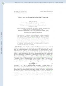
Thus, for large t, Var(N(0,t] ) is not constant but is periodic in t with period 1. The first term in (2.10) is just the variance of the rigid lattice. The second term goes to zero as α % ∞, when the process tends to that of the lattice, and goes to infinity as α & 1, when the process becomes Poisson; see Figure 1. The average W of W (θ) over the interval 0 ≤ θ ≤ 1 is, from (refbeta),  1  , as α & 1,  1 4 (α − 1)2 W = + '  6 log2 β 1 + 4 , as α % ∞. 6 α2

Large deviations for a point process

241

In terms of Y (t), the limit α & 1 corresponds to an unbinding transition: for any t, Y (t) % ∞ with probability 1 as α & 1.

α = 101 α = 11 α=2 α = 1.1 α = 1.01 α = 1.0 (Poisson)

Figure 1. Sample configurations of the G process at density ρ¯ = 1 in an interval of size L = 140, for α = 1.0 (the Poisson process) and α = 1 + 10 k , k = −2, −1, 0, 1, 2.

3. Large deviations In the introduction we discussed briefly the problem of large deviations for the number of points of a point process in an interval. We will return to this question in Section 4, but we must first consider the sharper problem of large deviations in the density profile exhibited by the process. Suppose then that we are given a nonnegative integrable function ρ(x) on the unit interval [0, 1]. We are interested in the event that the macroscopic empirical density profile — the coarse-grained and rescaled density for the point process in the region [0, L] (where L is considered to be very large) — agrees, approximately, with the function ρ(x), i.e. that, roughly, N(0,xL] ∼ L

Zx

ρ(ξ) dξ

for all x in [0, 1].

(3.1)

0

We say that the process satisfies a large deviation principle if the probability of the event (refseerho) decays with L as exp[−LG(ρ)] for some rate function G.

242

S. Goldstein, J.L. Lebowitz and E.R. Speer

We will refer to the given function ρ(x) as a density profile. Since the G process has density 1, the typical macroscopic empirical density profile will be approximately given by the constant density profile ρ(x) = 1; we are asking about the probability of seeing significant deviation from this behavior. One way to formalize this notion is to demand that   Zx −1 1 log Prob sup L N(0,xL] − ρ(ξ) dξ < ε = −G(ρ). lim lim ε→0 L→∞ L 0≤x≤1

(3.2)

0

In Theorem 3.3 below we give a slightly weaker version of (3.2) for the G process, in which the L → ∞ limit is replaced by either a lim sup or a lim inf. For the G process we may, by (2.1), restate (3.2) as  1 1 log Prob sup Y (xL) lim lim ε→0 L→∞ L 0≤x≤1 L    Zx 1 − Y (0) + (1 − ρ(ξ)) dξ < ε = −G(ρ). (3.3) L 0

We will approach (3.3) by first obtaining a large deviation principle for the probability that the rescaled Y process L−1 Y (xL) be uniformly close to some specified function y(x). It is this problem which we discuss next. We first describe precisely the probability space on which our processes are most conveniently regarded as defined. Since (3.2) involves N(0,t] only for t ≥ 0 we may realize the relevant part of the G process as the jumps of the process Yλ0 introduced in Section 2; here and below we write Yλ0 (t) ≡ Y (t). These ˆ with rate α > 1; jump points are a subset of the points of a Poisson process N ˆ this process is (for any α > 0) defined on the space Ω of locally finite point ˆ with configurations in (0, ∞) and is given by a probability measure νˆ on Ω, ˆ ˆ in the distribution of NI (ω), the number of points of the configuration ω ∈ Ω k ˆ the interval I, satisfying νˆ(NI = k) = (α|I|) exp(−α|I|)/k!. Y is then defined ˆ with measure ν = λ0 × νˆ by the on the probability space Ω ≡ (−1, ∞) × Ω conditions (i) Y (v, ω)(t) is right continuous, with left-hand limits, in t; (ii) Y (v, ω)(0) = v; (iii) (dY (v, ω)/dt)(t) = 1 unless t ∈ ω; (iv) if t ∈ ω, then Y (v, ω)(t) = Y (v, ω)(t−) − 1 unless Y (v, ω)(t−) ≤ 0, in which case Y (v, ω)(t) = Y (v, ω)(t−). In this context we formulate the problem posed at the end of the previous paragraph as follows. Let D denote the space of real-valued cadlag functions —

Large deviations for a point process

243

functions which are right continuous with left-hand limits at each point — on [0, 1], furnished with the Skorohod topology [16]. Then with ΦL : Ω → D defined by ΦL (v, ω)(x) = L−1 Y (v, ω)(Lx), we want to determine the L → ∞ asymptotics of the probability ν(Φ−1 L (S)) for open and closed subsets S ⊂ D. In particular the specific question raised below (3.3), which involves uniform neighborhoods of the continuous function y(x), can be answered in terms of Skorohod neighborhoods, since every Skorohod neighborhood of y contains a uniform neighborhood, and vice versa. We will adopt the standard terminology of the theory of large deviations [17]. Let X be a topological space. A function F : X → [0, ∞] is a good rate function on X if it is lower semicontinuous (l.s.c.) and the level sets F −1 ([0, a]), a ∈ R+ , are compact. A family {µL }L≥0 of Borel measures on X satisfies the large deviation principle (LDP ) with rate function F if 1 ˆ log µL (S) ≥ − inf F(y), y∈S L 1 ˆ lim sup log µL (S) ≤ − inf F(y), y∈S L→∞ L lim inf L→∞

if S ⊂ X is open,

(3.4)

if S ⊂ X is closed.

(3.5)

ˆ itself, for any α > 0, The large deviation theory for the Poisson process N ˆL : Ω ˆ →D may be conveniently stated in this framework. For L > 0 define Φ ˆ L (ω)(x) = x − L−1 N ˆ(0,Lx] ; note that we consider sample paths which, in by Φ parallel with those of the Y process, drift upward at unit velocity and take downward jumps at points of the Poisson process. We write AC for the set of absolutely continuous paths in D, and define the rate function Fˆ : D → [0, ∞] by  1 Z    g(1 − y 0 (x)) dx, if y ∈ AC, y(0) = 0, and y 0 (x) ≤ 1 a.e., ˆ (3.6) F(y) =  0   ∞, otherwise, where

g(r)(= gα (r)) = r log

r − r + α. α

(3.7)

Theorem 3.1. For any α > 0, Fˆ is a good rate function on D and the measures ˆ −1 on D satisfy the LDP with rate function F. ˆ νˆ ◦ Φ L Proof. This result is an easy consequence of Exercise 5.2.12 of [17]; in particular, ˆ −1 , regarded there as measures on L∞ ([0, 1]), are supported the measures νˆ ◦ Φ L on D and are Borel measures there. 2 Now we formulate the corresponding result for the G process. The rate function F(y), for which (essentially) −LF(y) is the log of the probability that

244

S. Goldstein, J.L. Lebowitz and E.R. Speer

the rescaled Y process ΦL (x) = L−1 Y (Lx) follows the path y(x) in D, is Z   g(1 − y 0 (x)) dx, if y ∈ AC, y ≥ 0, y(0) | log β| + F(y) = and y 0 (x) ≤ 1 a.e., { x∈[0,1]|y(x)>0 }   ∞, otherwise. (3.8) This formula may be understood intuitively as follows. First, F(y) is finite only if y ≥ 0 because Y > −1 and hence ΦL (x) > −1/L. Second, during any time interval in which Y (t) is strictly positive the Poisson and G processes are the same, and the contribution of such an interval to the rate function for the G process should correspond to (3.6); on the other hand, wherever Y (t) is nonpositive the Poisson process is free to produce points at its natural rate α, so the contribution to the rate function from such a region should vanish. Finally, the term y(0)| log β| arises from (2.3) as the cost of “preparing” the system at time 0 with L−1 Y (0) ∼ y(0). More formally, we will establish a result parallel to Theorem 3.1; the proof is given in Section 5. Theorem 3.2. For any α > 1, F is a good rate function on D, and the measures ν ◦ Φ−1 L on D satisfy the LDP with rate function F. The rate function G(ρ) for a density profile ρ ∈ L1 ([0, 1]), ρ ≥ 0, is now obtained via G(ρ) ≡ inf F(y), (3.9) y∈Jρ

0

where Jρ ≡ {y ∈ AC | y = 1 − ρ}; from (3.8) it follows that the infimum in (3.9) is achieved for y = yρ , with yρ (x) ≡

Zx




1 − ρ(ξ) dξ − 0 inf

0

x ∈[0,1]

Zx 0

0


1 − ρ(ξ) dξ.

We justify (3.9) by proving a version of equation (3.2): Theorem 3.3. Suppose that ρ ∈ L1 ([0, 1]) with ρ ≥ 0 and that for ε > 0, EL,ε (ρ) ⊂ Ω is the event that Zx −1 sup L N(0,xL] − ρ(t) dt ≤ ε.

0≤x≤1

Then lim lim inf

ε→0 L→∞

0

1 1 log ν(EL,ε (ρ)) = lim lim sup log ν(EL,ε (ρ)) = −G(ρ). ε→0 L→∞ L L

Large deviations for a point process

245

The proof is given in Section 5. In fact, (3.2) can also be proven, but the proof is considerably more complicated than that of Theorem 3.3 and provides no better justification of the interpretation of G. Remark 3.1. As indicated in the introduction, the G process studied here is a special case of the self-correcting processes of Isham and Westcott [1]. In the more general model the points of the process are again the jump points of an auxiliary process Y (t). For the density 1 case Y again increases at rate 1 except at its jump points, and these occur randomly at rate γ(Y (t)) for some specified nonnegative function γ. The G process is obtained by taking γ(v) = α for v > 0 and γ(v) = 0 for v ≤ 0. More generally, [1] requires that lim supv→−∞ γ(v) < 1 and lim inf v→∞ γ(v) > 1 and that γ(v) be strictly bounded away from 0 for v > 0. We expect that these processes will satisfy a large deviation principle in D whenever α± ≡ limv→±∞ γ(v) exist, with rate function similar to that of the G process (see (3.8): finite only for y ∈ AC with y 0 ≤ 1 and, for such y, Z F(y) = |y(0) log βsgn y(0) | + gα+ (1 − y 0 (x)) dx { y(x)>0 }

+

Z

gα− (1 − y 0 (x)) dx,

(3.10)

{ y(x) 0, pL (κ) ≡ 1, (4.1) if κ = 0 
 ν N(0,L] ≤ (1 + κ)L , if − 1 ≤ κ < 0,

Consider first κ ≥ 0. By (2.1), N(0,L] ≥ (1 + κ)L if and only if Y (L) ≤ Y (0) − κL; setting S0 = D and Sκ = {y ∈ D | y(1) ≤ y(0) − κ} for κ > 0 we see that pL (κ) = ν(Φ−1 L (Sκ )). Let ψ(κ) ≡ inf y∈Sκ F(y); we will compute ψ(κ) below and show that it is continuous for κ ≥ 0. Since for any ε > 0, Sκ+ε is contained in the interior of Sκ , Theorem 3.2 implies that −ψ(κ) ≥ lim sup log pL (κ) ≥ lim inf L→∞

L→∞

1 log pL (κ) ≥ −ψ(κ + ε). L

246

S. Goldstein, J.L. Lebowitz and E.R. Speer

Since ε is arbitrary, lim

L→∞

1 log pL (κ) = −ψ(κ). L

(4.2)

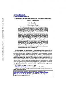
A similar argument shows that (4.2) holds also for −1 ≤ κ < 0, with ψ(κ) ≡ inf y∈Sκ F(y), where Sκ = {y ∈ D | y(1) ≥ y(0) − κ}. We next compute ψ(κ) = inf Sκ F(y). Certainly ψ(0) = inf D F = 0; the infimum is obtained by the function y ≡ 0. In general, since if y ∈ D is nonnegative, F(y) ≥ F(y − inf y), and since if y ∈ Sκ then also y − inf y ∈ Sκ , in computing inf Sκ F we need only consider nonnegative functions y in Sκ which vanish at some point. We now take κ > 0 and determine the function y ∈ Sκ which realizes inf Sκ F. Let a = inf{x ∈ [0, 1] | y(x) = 0}. From (3.8), y must vanish on [a, 1], and by the convexity of g and Jensen’s inequality, y must be affine on [0, a]; thus, setting y(0) = b, h  a + b i . (4.3) ψ(κ) = inf b | log β| + ag 0≤a≤1, a κ≤b Since g ≥ 0, ψ(κ) ≥ κ| log β|, and since g(α) = 0, this minimum is achieved when κ ≤ α − 1 by taking b = κ and (a + b)/a = α, i.e., a = κ/(α − 1). When κ > α − 1 the minimum for fixed a is achieved at b = κ, since g is increasing on [α, ∞), and the global minimum ψ(κ) = κ| log β| + g(1 + κ) is then at a = 1. The minimizing function y is shown in Figure 2.

Figure 2. Function y(x) minimizing F(y) subject to y(1) ≤ y(0) − κ, for κ ≥ 0. The analysis for −1 ≤ κ < 0 begins in a similar way. The minimizing y in Sκ must vanish on some interval [0, a] and be affine, with y 0 ≤ 1, on [a, 1], and

Large deviations for a point process

b = y(1) must satisfy b ≥ |κ|, so that h  1 − a − b i ψ(κ) = inf (1 − a)g . 0≤a≤1−|κ| 1−a |κ|≤b≤1−a

247

(4.4)

Since g is decreasing on [0, α] the minimum for fixed a ≤ 1 − |κ| is at b = |κ|. For |κ| ≤ 1 − αβ the global minimum ψ(κ) = |κ|| log β| is achieved at a = (1 − αβ − |κ|)/(1 − αβ); for |κ| > 1 − αβ the global minimum ψ(κ) = g(1 + κ) is achieved at a = 0; see Figure 3. Thus   if − 1 ≤ κ ≤ αβ − 1, g(1 + κ), (4.5) ψ(κ) = |κ|| log β|, if αβ − 1 ≤ κ ≤ α − 1,   κ| log β| + g(1 + κ), if α − 1 < κ.

Figure 3. Function y(x) minimizing F(y) subject to y(1) ≥ y(0) − κ, for κ ≤ 0. Remark 4.1. Formula (4.5) for κ < 0 can perhaps be better understood by considering the time reversal of the Y process with respect to the stationary measure with density given in (2.3). This process involves unit jumps upward at the rate αβ, yielding ( |κ|| log β| + gαβ (1 + κ), if − 1 ≤ κ < αβ − 1. (4.6) ψ(κ) = |κ|| log β|, if αβ − 1 ≤ κ ≤ 0, which agrees with (4.5); gαβ was defined in (3.7). (In more detail: the reversed process drifts downward with unit velocity and takes unit jumps upward, at rate αβ when y > 0 and at rate α(1 − β)β y+1 /(1 − β y+1 ) when −1 < y ≤ 0.)

248

S. Goldstein, J.L. Lebowitz and E.R. Speer

We may compare (4.5) with the corresponding result for the Poisson process ∗ of density 1. Defining p∗κ (L) as in (4.1) but with N(0,L] replaced by N(0,L] , the number of points of this process in (0, L], we have lim

L→∞

1 log p∗κ (L) = ψ ∗ (κ) ≡ g1 (1 + κ), L

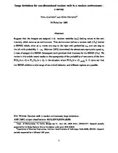
where g1 is defined in (3.7). This follows from a simple computation with Stirling’s formula; it may also be obtained from Theorem 3.1, and we then find that the minimizing y ∗ ∈ D is y ∗ (x) = −κx, corresponding to constant density 1 + κ for the points of the Poisson process. Figure 4 compares ψ and ψ ∗ .

Figure 4. Rate functions for the event N(0,L] ∼ (1 + κ)L: ψ(κ) for the G process (solid line) and ψ ∗ (κ) for the Poisson process (dashed line). One may also ask a related question, for either the Poisson or the G process: what is the rate function for the probability of a constant density profile ρ(x) = 1+κ (which of course gives rise to (1+κ)L points in the interval (0, L]; compare (4.1)? For the Poisson process of rate 1 this is just g1 (1 + κ), since, as remarked above, the constant profile is the typical one when we condition on the total number of particles in the interval. For the G process, however, the rate function is ψ0 (κ) ≡ G(ρ) as obtained from (3.9), which yields   if − 1 ≤ κ < 0; g(1 + κ), ψ0 (κ) = 0, (4.7) if κ = 0,   κ| log β| + g(1 + κ)(= gαβ (1 + κ)), if 0 < κ. Since g(1) = α − 1 − log α > 0, ψ0 (κ) is nonconvex and discontinuous at κ = 0. See Figure 5.

Large deviations for a point process

249

Figure 5. Rate function ψ0 (κ) for the event ρ(x) ∼ (1 + κ), 0 ≤ x ≤ 1, in the G process. 5. Proofs of the main results We will prove Theorem 3.2 via the contraction principle [17]: if X and Y are Hausdorff spaces, {µL } is a family of Borel measures on X satisfying the LDP with good rate function F, and f : X → Y is continuous at each point x ∈ X for which F(x) < ∞, then the family {µL ◦ f −1 } satisfies the LDP on Y with ¯ good rate function F(y) = inf x∈f −1 (y) F(x). To proceed we first derive an LDP for a family of measures on D obtained from those of the Poisson process. Define Φ0L : R → R by Φ0L (v) = v/L; it is easy to see that if F0 : R → [0, ∞] is defined by ( a | log β|, if a ≥ 0, F0 (a) = ∞, if a < 0, then the measures λ0 ◦ Φ−1 0L on R satisfy the LDP with rate function F0 . Now ˜ L : Ω → D by Φ ˜ L (v, ω)(x) = Φ0L (v) + Φ ˆ L (ω)(x) and F˜ : D → [0, ∞] define Φ ˜ ˆ by F(y) = F0 (y(0)) + F(y − y(0)). Finally, let P ⊂ D be defined by P = S ˜ ¯ L≥1 ΦL (Ω) and let P be the closure of P in D.

˜ −1 (P )) = ν(Φ ˜ −1 (P¯ )) = 1 for all L ≥ 1. Remark 5.1. We note that (i) ν(Φ L L ¯ Clearly, any function z ∈ P satisfies z(x2 ) − z(x1 ) ≤ x2 − x1

whenever 0 ≤ x1 ≤ x2 ≤ 1;

(5.1)

250

S. Goldstein, J.L. Lebowitz and E.R. Speer

conversely, (ii) any continuous function z on [0, 1] which satisfies (5.1) may be ˜ L (Ω), and hence uniformly approximated, to accuracy 1/L, by functions in Φ belongs to P¯ , since one may apply to z˜, where z˜(t) = z(t) − t, the simple fact that any continuous nonincreasing function can be uniformly approximated, to accuracy 1/L, by a piecewise constant function whose jumps are down and of size 1/L. ˜ −1 on D, and on P¯ , satisfy the LDP with good Lemma 5.1. The measures ν ◦ Φ L ˜ rate function F. ˆ −1 ) satisfy the large deviation Proof. The product measures (λ0 ◦ Φ−1 ν ◦Φ 0L ) × (ˆ L ∗ ˆ principle on R × D with good rate function F (a, y) = F0 (a) + F(y) (see [17]; the proof uses the fact that R and D are Polish spaces). The large deviation ˜ −1 on D is obtained from an application of the contraction principle for ν ◦ Φ L principle to the map f : R × D → D defined by f (a, y) = a + y. The LDP on P¯ follows at once from Remark 5.1(i) and the observation that ¯ ˜ y ) < ∞ }, an immediate consequence Remark 5.1(ii). P contains { y˜ ∈ D | F(˜ 2 ˜ L , of Ω into D, Now for each L ≥ 1 we have defined two maps, ΦL and Φ obtained from the G process and the Poisson process, respectively. The next lemma relates them by a map to which we can apply the contraction principle. Lemma 5.2. There exists a map f : P¯ → D such that ˜ L; (a) for every L ≥ 1, ΦL = f ◦ Φ ˜ y ) < ∞ then f is continuous at y˜; (b) if y˜ ∈ P¯ and F(˜ ˜ y ). (c) if y ∈ D then F(y) = inf y˜∈f −1 (y) F(˜ Proof of Theorem 3.2. The theorem follows immediately from Lemma 5.1 and Lemma 5.2, and the contraction principle. 2 Before proving Lemma 5.2 we establish two technical lemmas, for which we need the following definitions. First, if y ∈ D is lower semicontinuous (which means that y(x−) ≥ y(x) for all x ∈ (0, 1]) then we define Ky ⊂ D to be the set of all y˜ such that y˜(0) = y(0) and such that φ(x) ≡ y(x) − y˜(x)

(5.2)

is nondecreasing on [0, 1] and is locally constant on the (open) set { x ∈ [0, 1] | y(x) > 0 }. Second, we let H be the space of strictly increasing, continuous, and onto functions h : [0, 1] → [0, 1], for h ∈ H set  h(x ) − h(x )  1 2 khk = sup log , x1 − x 2 x1 6=x2

Large deviations for a point process

251

and for y, z ∈ D define d(y, z) = inf max{khk, ky − z ◦ hk∞ }. h∈H

Then d is a metric for D and in this metric D is complete [16]. Lemma 5.3. Suppose that y1 , y2 ∈ D are l.s.c., that y˜i ∈ Kyi for i = 1, 2, and that for some ε > 0, (i) y1 , y2 > −ε and (ii) d(˜ y1 , y˜2 ) < ε. Then d(y1 , y2 ) < 3ε. Proof. By (ii) there is a h ∈ H with khk < ε and k˜ y1 −˜ y2 ◦hk∞ < ε. We will show below that that y1 (x)−y2 (h(x)) < 3ε for all x ∈ [0, 1]; interchanging the roles of y1 and y2 and replacing h by h−1 we then have that also y2 (x)−y1 (h−1 (x)) < 3ε for all x, so that y2 (h(x)) − y1 (x) < 3ε for all x and hence ky1 − y2 ◦ hk∞ < 3ε. Now we fix x ∈ [0, 1] and show that y1 (x) − y2 (h(x)) < 3ε. If y1 > 0 on [0, x] then set x∗ = 0. Otherwise, define x∗ = sup{ t ∈ [0, x] | y1 (t) ≤ 0}; since y1 is l.s.c. and cadlag, y1 (x∗ ) = 0 in this case. Then from (5.2) and hypotheses (i) and (ii) we have, with φi = yi − y˜i , i = 1, 2, as in (5.2),

y1 (x) − y2 (h(x)) = y1 (x∗ ) − y2 (h(x∗ )) + y˜1 (x) − y˜2 (h(x))

− y˜1 (x∗ ) − y˜2 (h(x∗ )) + φ1 (x) − φ1 (x∗ )
− φ2 (h(x)) − φ2 (h(x∗ )) < ε + ε + ε + 0 + 0.

(5.3)

Note that the first term in (5.3) is bounded by ε from hypothesis (ii) if x∗ = 0 and from hypothesis (i) otherwise, and that φ1 (x) = φ1 (x∗ ) because if x > x∗ then y1 is strictly positive on (x∗ , x] and φ1 is right continuous. 2 Lemma 5.4. If y ∈ D is nonnegative and l.s.c., and some y˜ ∈ Ky is absolutely continuous, then y is also absolutely continuous. Proof. For any ε > 0 there is a δ > 0 such that if { [ui , vi ] | i = 1, . . . , n } is a collection of nonoverlapping intervals of total length less than δ then X |˜ y (vi ) − y˜(ui )| < ε. (5.4) i

But then also

X

|y(vi ) − y(ui )| < ε.

(5.5)

i

To see this, note that if y does not vanish on [ui , vi ] then y(vi ) − y(ui ) = y˜(vi ) − y˜(ui ), and if it does then |y(vi ) − y(ui )| ≤ |y(vi ) − y(vi0 )| + |y(u0i ) − y(ui )|,

252

S. Goldstein, J.L. Lebowitz and E.R. Speer



where u0i = inf {y = 0} ∩ [ui , vi ] and vi0 = sup {y = 0} ∩ [ui , vi ] . But since |y(vi ) − y(vi0 )| = |˜ y (vi ) − y˜(vi0 )| and |y(u0i ) − y(ui )| ≤ |˜ y (u0i ) − y˜(ui )|, we may then bound (5.5) by a sum of the form (5.4) for the collection of intervals in which [ui , vi ] is sometimes replaced by [ui , u0i ] and [vi0 , vi ]. 2 Proof of Lemma 5.2. The function f is unambiguously defined on P by condition (a). For each y˜ ∈ P which has at least one discontinuity is of the form ˜ L (v, ω) for a unique L and unique v = y˜(0)L, and ω ∩ (0, L] is uniquely deterΦ mined by y˜. We may then define f (˜ y ) = ΦL (v, ω), since this is determined by ω ∩ (0, L]. The exceptional (continuous) y˜ ∈ P are those of the form y˜ = za for ˜ L (aL, ω 0 ) for any L some a ∈ (−1, ∞), where za (x) ≡ a + x; note that za = Φ L 0 0 such that aL > −1, with ωL any point configuration satisfying ωL ∩ (0, L] = ∅. 0 In this case, however, ΦL (v, ωL ) = y˜ for all such L, so that we may define f (˜ y) = y˜ and satisfy (a). We remark that it is easy to see that y˜ ∈ K f (˜y) for all y˜ ∈ P . To extend f to P¯ we suppose that y˜ ∈ P¯ \ P and that y˜ = limn→∞ y˜n for ˜ Ln (Ω). Then necessarily limn→∞ Ln = ∞, for otherwise there would y˜n ∈ Φ exist L∗ , M < ∞ such that a subsequence of (˜ yn ) would belong to [ ˜ L (Ω) ∩ {z ∈ D | kzk∞ ≤ M }. Φ (5.6) 1≤L≤L∗

But (5.6) is easily seen to be compact, so that we would have y˜ ∈ P , a contradiction. From this and Lemma 5.3 it follows that the sequence f (˜ yn ) is Cauchy in D and we may thus define f (˜ y ) by f (˜ y ) = limn→∞ f (˜ yn ); it also follows easily that f (˜ y) is nonnegative and that f is continuous at y˜. The fact that Ln → ∞ also implies that y˜ and f (˜ y) are continuous; thus the convergence of y˜n and f (˜ yn ) is uniform [16] and from this and the fact that y˜ ∈ Kf (˜y) for y˜ ∈ P the same conclusion follows for y˜ ∈ P¯ . The function f satisfies (a) on P¯ since it does so on P . Since we know that f is continuous at all points of P¯ \ P we may verify (b) by showing that f is continuous at points of P at which F˜ is finite. These points are precisely the functions za with a ≥ 0, and it suffices to show that if za = limn→∞ y˜n with ˜ Ln (Ω) then limn→∞ f (˜ yn ) = f (za ) = za . In fact it suffices to consider y˜n ∈ Φ separately the cases Ln → ∞ and Ln bounded; the first of these is covered by the argument given above for y ∈ P¯ \ P , and the second is possible only if, for sufficiently large n, y˜n = zan with an → a; then f (˜ yn ) = zan → za = f (za ). We have seen that if y = f (˜ y) then y˜ ∈ Ky . Conversely, when y and y˜ are absolutely continuous, and y is nonnegative with y 0 ≤ 1 a.e., we have that if y˜ ∈ Ky then y = f (˜ y ). For given ε > 0 we may by (5.2) and Remark 5.1(ii) approximate y˜ to within ε by a function y˜∗ ∈ ΦL (Ω) with L > 1/ε, and it follows then from Lemma 5.3 that d(f (˜ y ), f (˜ y ∗ )) < 3ε and d(f (˜ y ∗ ), y) < 3ε. Note in particular that y = f (y) in this case.

Large deviations for a point process

253

We finally verify property (c). If y ∈ D is negative at some point then F(y) = ∞; if also y = f (˜ y ) then either y = y˜ = za with a < 0 or y˜ is discontinuous, ˜ y ) = ∞. If y is nonnegative and not absolutely continuous and in either case F(˜ ˜ y ) < ∞. then F(y) = ∞, and by Lemma 5.4 we cannot have y = f (˜ y ) with F(˜ Suppose then that y is nonnegative and absolutely continuous. If y 6= f (˜ y ) for any y˜ then we cannot have y 0 ≤ 1 a.e., since otherwise y = f (y); thus F(y) = ∞ in this case. Finally, suppose that y = f (˜ y ) for some y˜ (which implies that y 0 ≤ 1 ˜ y ), for if F(˜ ˜ y ) = ∞ this is trivial, while if F(˜ ˜ y) < ∞ a.e.). Then F(y) ≤ F(˜ then since y˜ ∈ Ky , ˜ y ) = y˜(0)| log β| + F(˜

Z1

g(1 − y˜0 (x)) dx

0

≥ y˜(0)| log β| +

Z

g(1 − y˜0 (x)) dx

{ y>0 }

= F(y). ˜ y ). On the other hand, for this y we may define Thus F(y) ≤ inf y˜∈f −1 (y) F(˜ y˜ = y − φ with φ(0) = 0 and ( 0, if y(x) > 0, φ0 (x) = (5.7) α − 1, if y(x) = 0. ˜ y ) = F(y) and f (˜ Then F(˜ y) = y, since y 0 ≤ 1 a.e. This completes the verification of (c). 2 Remark 5.2. ODE There is another way to complete the proof of Lemma 5.2, after defining f on P as above. If z is a real-valued function of bounded variation we will write z = z+ − z− for the canonical decomposition of z as the difference of two increasing functions, so that dz = dz+ − dz− is the Hahn decomposition of the signed measure dz as the difference of two nonnegative measures; note ˜ L (v, ω) ∈ P then y˜ is of bounded variation, with d˜ that if P y˜ = Φ y+ = dx, d˜ y− = {x|Lx∈ω} L−1 δx . Now it is easy to verify that for y˜ ∈ P , y ≡ f (˜ y) satisfies the integral equation y(x) = y˜(0) +

Zx

[d˜ y+ − χy d˜ y− ],

(5.8)

if y(x−) > 0, if y(x−) ≤ 0.

(5.9)

0

where χy (x) =

(

1, 0,

254

S. Goldstein, J.L. Lebowitz and E.R. Speer

But one may also show directly that (5.8)–(5.9) has a unique solution y whenever y˜ is continuous, of bounded variation, and satisfies y˜(0) ≥ 0. Taking this solution as the definition of f (˜ y) = y when y˜ ∈ P¯ \ P , one verifies the properties of Lemma 5.2. Finally, we give the Proof of Theorem 3.3. From (2.1),
∞ EL,ε (ρ) = Φ−1 L Bε (Jρ ) ,

where Jρ was defined below (3.9) and Bε∞ denotes an ε-ball in the uniform metric on D. Because each y ∈ Jρ is a translate of the continuous function yρ , however, there is a δ > 0 such that Bδ (Jρ ) ⊂ Bε∞ (Jρ ); then by Theorem 3.2, lim inf L→∞


1 1 log ν(EL,ε (ρ)) ≥ lim inf log ν Φ−1 L (Bδ (Jρ )) L→∞ L L ≥ −F(yρ ) = −G(ρ),

and hence lim inf lim inf ε→0

L→∞

1 log ν(EL,ε (ρ)) ≥ −G(ρ). L

(5.10)

Conversely, since Bε∞ (Jρ ) ⊂ Bε (Jρ ) ⊂ Bε (Jρ ), F is l.s.c., and for y ∈ Bε (yρ ), F(y + c) − F(yρ + c) is independent of c for c > ε, lim sup lim sup ε→0

L→∞


1 1 log ν(EL,ε (ρ)) ≤ lim sup lim sup log ν Φ−1 L (Bε (Jρ )) L ε→0 L→∞ L ≤ − lim inf inf F(y) ε→0

y∈Bε (Jρ )

= − inf F(y) = −G(ρ). y∈Jρ

Equations (5.10) and (5.11) together imply (3.3).

(5.11) 2

Added note After this work was completed we were informed by Neil O’Connell that our large deviation result for the G process could be deduced from the results in the paper of A.A. Puhalski and Ward White, Functional Large Deviation Principles for Waiting and Departure Processes, Probability in the Engineering and Informational Sciences 12, 479–507, 1998. The purpose of that paper, which is part of a series, is “to establish large deviation principles for waiting and departure processes in single-server queues . . . ”. The focus of our paper, the statistical mechanics of point processes with bounded variability, is quite different, and should be of independent interest.

Large deviations for a point process

255

Acknowledgments We thank Ofer Zeitouni for a helpful suggestion and Neil O’Connell for pointing out the connection of the G process to queueing theory. The work of J.L.L. was supported by NSF Grant DMR 01–279–26 and AFOSR Grant AF 49620–01–1–0154, and DIMACS and its supporting agencies. The work of S.G. was supported in part by NSF Grant DMS 0504504. E.R.S. thanks the Institute for Advanced Study, and all the authors thank the Institut des Hautes Etudes Scientifique, for hospitality while parts of this work were carried out. References [1] V. Isham and M. Westcott (1979) A self-correcting point process. Stoch. Proc. Appl. 8, 335–247. [2] T. Lewis and L. J. Govier (1964) Some properties of counts of events for certain types of point processes. J. Roy. Statist. Soc. Ser. B 26, 325–337, and references therein. [3] D.J. Daley (1971) Weakly stationary point processes and random measures. J. Roy. Statist. Soc. Ser. B 33, 406–428. ´ cs and D. Sza ´ sz (1975) On a problem of Cox concerning point process in [4] P. Ga Rk of “controlled variability”. Ann. Prob. 3, 597–607. [5] M. Aizenman, S. Goldstein and J.L. Lebowitz (2001) Bounded fluctuations and translation symmetry breaking in one-dimensional particle systems. J. Stat. Phys. 103, 601–618. [6] M. Yamada (1961) Geometrical study of the pair distribution function in the many-body problem. Prog. Theor. Phys. 25, 579–594. [7] A. Gabrielli, B. Jancovici, M. Joyce, J. L. Lebowitz, L. Pietronero and F. Sylos Labini (2003) Generation of primordial cosmological perturbations from statistical mechanical models. Phys. Rev. D 67, 043506:1–7. [8] J. Beck (1987) Irregularities of distribution: I. Acta Math. 159, 1–49. [9] S. Torquato and F.H. Stillinger (2003) Local density fluctuations, hyperuniformity, and order metrics. Phys. Rev. E 68, 041113:1–25. [10] J.L. Lebowitz (1983) Charge fluctuations in Coulomb systems. Phys. Rev A 27, 1491–1494. [11] D. Levesque, J.-J. Weis and J.L. Lebowitz (2000) Charge fluctuations in the two-dimensional one-component plasma. J. Stat. Phys. 100, 209–222. [12] M.L. Mehta (1991) Random Matrices. Academic Press, New York. [13] K. Johannson (2003) Determinental processes with number variance saturation. Preprint arXiv:math.PR/0404133 v1 6 April. [14] B. Jancovici, J.L. Lebowitz and G. Magnificat (1993) Large charge fluctuations in classical Coulomb systems. J. Stat. Phys. 72, 773–787.

256

S. Goldstein, J.L. Lebowitz and E.R. Speer

[15] S. Asmussen (2003) Applied Probability and Queues. Springer, New York. [16] P. Billingsley (1968) Convergence of Probability Measures. John Wiley & Sons, Inc., New York. [17] A. Dembo and O. Zeitouni (1998) Large Deviations: Techniques and Applications. Springer, New York.