Large deviations in weakly interacting boundary driven lattice gases

arXiv:cond-mat/0404358v1 [cond-mat.stat-mech] 15 Apr 2004

Large deviations in weakly interacting boundary driven lattice gases

Fr´ed´eric van Wijland1,2 and Zolt´an R´acz1,3 1

Laboratoire de Physique Th´eorique, Bˆat. 210, Universit´e de Paris-Sud, 91405 Orsay Cedex, France. 2

Pˆole Mati`ere et Syst`emes Complexes, Universit´e de Paris VII, France.

3

Institute for Theoretical Physics, HAS Research Group, E¨otv¨os University 1117 Budapest, P´azm´any s´et´any 1/a, Hungary.

Abstract One-dimensional, boundary-driven lattice gases with local interactions are studied in the weakly interacting limit. The density profiles and the correlation functions are calculated to first order in the interaction strength for zero-range and short-range processes differing only in the specifics of the detailed-balance dynamics. Furthermore, the effective free-energy (large-deviation function) and the integrated current distribution are also found to this order. From the former, we find that the boundary drive generates long-range correlations only for the shortrange dynamics while the latter provides support to an additivity principle recently proposed by Bodineau and Derrida.

1

1 Introduction One-dimensional boundary driven lattice gases are simple model systems which allow detailed studies of nonequilibrium steady-states. They are relevant in the sense that steady states in experiments are often produced by choosing appropriate boundary conditions (heating a horizontal layer of liquid from below being the most widely quoted example) and, furthermore, these models appear to capture some important consequences of the nonequilibrium drive such as e.g. the generation of long-range correlations. Analytical approaches to driven lattice gases proceed along two distinct paths. On one hand, exploiting the matrix product method, Derrida and coworkers [1, 2, 3, 4, 5, 6] have come up with a series of exact results for the exclusion process (hard-core particles undergoing symmetric or biased diffusive motion) in one dimension . On the other hand, in a parallel series of papers, Bertini and coworkers [7, 8, 9] solved some of the same problems employing the formalism of fluctuating hydrodynamics. The results obtained for the probability functional of a given density profile or for the integrated current distribution are important since they provide new insights into the properties of nonequilibrium steady states. Thus it would be highly desirable to establish how general or universal these results are. In order to investigate this generality issue, in this paper, we go beyond the specificity of the exclusion process, and study the effects of varying the interactions between the particles as well as varying the microscopic dynamics in boundary driven lattice gases. Our main ”technical” results are the derivation of the weak interaction limits of both the nonequilibrium free energy and the distribution of the integrated particle current. From the explicit form of the free energy, we can then deduce the density profile and the correlations (effective interactions) for various interactions (pair or triplet) and various dynamics [zero-range [10] and short-range (misanthropic [11]) processes]. Our main ”physical” findings are that the density profiles are nonlinear and they depend on both the interactions and the dynamics. Furthermore, the details of the dynamics are found to change the the correlations from short- to long-range, and they are shown to be able to change the sign of the effective interactions. As to the distributions of the integrated particle current, we verify that, for all the interaction- and dynamics combinations we studied, they are in agreement with the recently proposed addititvity principle which allows to construct this distribution function from the knowledge of its first two moments [12]. We start by introducing the models of interacting lattice gases and deriving dy2

namical rules satisfying detailed balance in the absence of boundary drive (Sec.2). Next we describe on the example of free particles how the models can be formulated in terms of field theories (Sec.3). Zero-range and short-range (misanthropic) processes are worked out in Sections 4 and 5, respectively. There we provide explicit expressions for the effective free energies. Finally, Sec.6 is devoted to a separate treatment of the integrated current distribution.

2 The model 2.1 Lattice gas with onsite interaction and boundary drive A d = 1 dimensional lattice gas is considered with hopping dynamics in the bulk and with particle injection and removal at the ends of the chain. The state of the system ~n ≡ {n0 , n1 , ..., nL } is specified by the number of particles ni = 0, 1, ..., ∞ at lattice sites i (i = 0, 1, ..., L), and the interactions are assumed to be local L X E(~n) = hi (1) i=0

where hi = h(ni ) is the energy of interactions among particles at the same site. We shall treat the simplest case of pair interactions, h(n) = εn(n − 1). However triplet interactions, h(n) = εn(n − 1)(n − 2), will also be considered occasionally either for demonstrating the effects of competing interactions hi = h(ni ) = ε (±ni (ni − 1) + λni (ni − 1)(ni − 2)) .

(2)

or for probing the universality of our results with respect to varying the type of interaction. For λ = 0, we restrict our study to the + sign in the r.h.s. of (2) in order to have stability against collapse of all particles on a single site, while for λ > 0 both signs will be considered. The dynamics of the system is described in terms of a master equation for the time evolution of the probability P (~n, t) of a given particle configuration ∂t P (~n, t) = LD P (~n, t) + LBC P (~n, t)

(3)

where the first and second terms on the right-hand side represent the nearestneighbor hopping in the bulk and the injection-removal terms at the boundaries.

3

The bulk term is given through the rate of hopping wi→i±1 (~n) from site i to i ± 1 in a state ~n as LD P (~n, t) = −

L−1 X

wi→i+1 (~n)P (~n, t) −

i=0

+

L−1 X

L X

wi→i−1 (~n)P (~n, t)

(4)

i=1

wi→i+1(~ni+1→i )P (~ni+1→i, t) +

i=0

L X

wi→i−1(~ni−1→i )P (~ni−1→i , t)

i=1

where state ~ni→j is obtained from ~n by moving a particle from i to j. The injection and removal of particles at the boundaries i = 0 and i = L are described by the terms   LBC P (~n, t) = − w0+ (~n) + wL+ (~n) + w0− (~n) + wL− (~n) P (~n, t) (5) − + + w0 (~n0− ) P (~n0− , t) + w0 (~n0+ ) P (~n0+ , t) + wL+ (~nL− ) P (~nL− , t) + wL− (~nL+ ) P (~nL+ , t) where w0+ (~n), w0− (~n), wL+ (~n) and wL− (~n) are the rates of adding (+) or removing (−) a particle at site 0 or L in the state ~n and, furthermore, the state ~ni+(−) is obtained from ~n by adding (removing) a particle at site i.

2.2 Choice of dynamics 2.2.1 Equilibrium distribution In order to specify the dynamics, we shall assume that if the injection and removal rates are such that there is not net flux (particle or energy current) through the system then equilibrium is reached. Due to the onsite nature of the interaction, the equilibrium distribution factorizes, it becomes the grand-canonical distribution Peq (~n) =

Y

peq (ni ),

peq (ni ) =

i

1 ζ ni e−hi /T Ξ ni !

(6)

where T and ζ are characterizing the temperature and fugacity of the outside heat and particle bath, and Ξ is a normalization factor. In the following, we shall absorb T in the interaction strength ε and the high temperature limit studied below will simply mean that ε is small.

4

2.2.2 Hopping rates The bulk hopping rates may now be defined by making the natural (though not necessary) assumption that they satisfy detailed balance with Peq , and that the detailed balance remains valid in the presence of the boundary drive, as well. This assumption yields the following condition for the rate of hopping to the right ni e−[E(~ni→i+1)−E(~n)]/2 wi→i+1 (~n) = wi+1→i (~ni→i+1 ) (ni+1 + 1)e−[E(~n)−E(~ni→i+1 )]/2 ni eh(ni )−h(ni −1) , = (ni+1 + 1)eh(ni+1 +1)−h(ni+1 )

(7) (8)

and similar condition with i + 1 replaced by i − 1 applies for the rate of hopping to the left. Clearly, the hopping rates are not uniquely determined by detailed balance. The remaining arbitrariness is not relevant for equilibrium but, in the presence of a drive, the steady state properties do depend on details of the dynamics. In order to have some idea about the importance of various choices, we shall consider two significantly different rates. First, the rates will be chosen so that they depend only on the energy change at the site from which the hopping originates. As can be seen from (8), a choice satisfying this condition is as follows (zr)

wi→i+1 (~n) = Dni eh(ni )−h(ni −1)

(9)

where D is the ”diffusion coefficient” setting the timescale. Dynamics defined by the above rate is an example of the so called zero range processes [10, 13] where, in general, the rate is an arbitrary function of ni . Thus, the first half of our study can be viewed as an investigation of zero range processes in the presence of a boundary drive. For a second choice, a more standard hopping dynamics will be used with rates depending not only on the energy change at the starting position of the hopping particle but on the total energy change due to the hopping. This choice follows from the eq.(7) version of detailed balance (sr)

wi→i+1 (~n) = Dni e−[h(ni −1)+h(ni+1 )−h(ni )−h(ni+1 )]/2

(10)

where a subscript in w (sr) signifies the name short range process [11] we shall use in order to distinguish the resulting dynamics from the zero range process. An important feature of the short range process is that tuning the interactions 5

(0 ≤ ε < ∞, λ = 0) so that one extrapolates between the exactly solvable noninteracting limit (ε = 0) and the much investigated and also exactly solvable [1, 9] boundary driven symmetric exclusion process (ε → ∞). 2.2.3 Boundary drive (injection and removal rates) Nonequilibrium drive is introduced into the model through injection and removal of particles at the ends (j = 0 and L) of the chain. The rates can be set again by referring to detailed balance condition with the baths attached to the ends of the chain. The baths are assumed to contain noninteracting particles with the chemical potentials set to produce the appropriate injection and removal rates. For zero range process, the removal can be imagined as diffusion into the baths. The rates are independent of the properties of the baths and given by (9) with D replaced by new (externally controlled) parameters β and γ, yielding (zr)−

w0

(~n) = γn0 eh(n0 )−h(n0 −1)

(zr)−

;

wL

(~n) = βnLeh(nL )−h(nL −1) .

(11)

Within the picture of zero range process, the injections (moving a particle from the bath to the end sites) are independent of state of the end sites, and thus they are constants α and δ determined by the properties of the baths (zr)+

w0

(~n) = α

(zr)+

;

wL

(~n) = δ .

(12)

The boundary rates for the short range process are determined along similar lines. The rate of removal follows from (7) and, since the particles in the baths are not interacting, they are given by (sr)−

w0

(~n) = γn0 e[h(n0 )−h(n0 −1)]/2

;

(sr)−

wL

(~n) = βnL e[h(nL )−h(nL −1)]/2 . (13)

In order to satisfy the detailed balance (7), the injection rates must also depend on the energy change due to the adding a particle and, using again that the particles in the bath do not interact, we find (sr)+

w0

(~n) = αe[h(n0 )−h(n0 +1)]/2

;

(sr)+

wL

(~n) = δe[h(nL )−h(nL +1)]/2 .

(14)

We have now finished the description of the two models we shall be concerned with in this paper. Eqs. (9,11,12) define the boundary driven zero range process while the rates given by eqs. (10,13,14) define the corresponding short range process. As one can easily verify, the case of α δ = γ β 6

(15)

corresponds to equilibrium with the baths (no drive) and the steady state distribution is the equilibrium distribution given by eq.(6). Nonequilibrium drive is present when the above equality is violated.

3 Preparing for the perturbation expansion: Noninteracting particles 3.1 From the master equation to path integrals We shall now perform the mapping of the master equation for the probability that the system is in the occupation numbers configuration ~n at time t, namely, P (~n; t), to a field theory, where approximation techniques inherited from our experience with equilibrium systems can be transferred without any difficulty. We only briefly sketch theP procedure (see [14] for a recent review). We build up the state vector |Ψ(t)i = ~n P (~n, t)|~ni and rewrite the master equation for P in terms of and evolution equation for |Ψ(t)i. This equation can be cast in the form d|Ψ(t)i = Lˆ0 |Ψ(t)i (16) dt where Lˆ0 is an evolution operator acting on the microstates |~ni indexed by the local particle numbers. Not suprisingly, the evolution operator Lˆ0 is conveniently expressed in terms of the creation and annihilation operators a†i , ai related to each local occupation number ni . For the rates specified in the previous subsection, but at ε = 0, it takes the following form X X † −Lˆ0 =D (ai − a†j )ai i

j nn of i

+ α(1 − a†0 ) + δ(1 − a†L )

(17)

+ γ(a†0 − 1)a0 + β(a†L − 1)aL One can of course recognize that at ε = 0 one is formally dealing with a free boson hamiltonian. The next step consists in converting the computation of expectation values of physical observables into the evaluation of a path-integral over two fields a ˆi (t) and ai (t). This step leads to averaging a physical observable A({ni }) in the following way: Z ˜ a(t)) e−Sε [ˆa,a] hA(~n)i = Dˆ ai Dai A(~ (18) 7

where S0 [ˆ a, a] = −

X i

ai (t) +

Z

t

dτ

0

hX

a ˆi ∂τ ai + D

i

X

(ˆ ai − aˆj )ai

j

+ α(1 − a ˆ0 ) + γ(ˆ a0 − 1)a0

+ δ(1 − aˆL ) + β(ˆ aL − 1)aL



(19)

i

Note that we have moved the initial condition to t = −∞, in order to sit directly in the steady-state (initial condition independent). The prescription to obtain A˜ is as follows: normal order A({a†i ai }) and then replace the operators a†i and ai ˜ a(t)). We have adopted a by the fields one and ai (t) respectively. This yields A(~ path-integral formulation because of the large toolbox that goes with it. Besides, it formally provides us with a sort of dynamical partition function on which series expansion are straightforward. The efficiency of the mapping lies in the following observation: at ε = 0, that is for independent particles, the Gaussian field theory exactly encodes Poissonian statistics. Hence the high-temperature (ε → 0) expansion that will be performed next consists in expanding around the Poissonian distribution. For free particles, as expected, the stationary measure factorizes as a product of local Poissonian distributions, P (~n) =

Y i

e−ζi

ζini ni !

(20)

Hence, for free particles, there is local equilibrium, and the density field ρi = hni i is identical to the fugacity field ζi . This means that the properties of the system are the same as those that one would obtain in equilibrium if one imposed a space dependent fugacity ζi . Here the explicit expression of the fugacity is given by, in the continuum limit, setting x = i/L ∈ [0, 1], ζ(x) = ζ0 + (ζ1 − ζ0 )x +

ζ0 − ζ1 (γx − β(1 − x)) + O(L−2 ) βγL

(21)

where we have set ζ0 = αγ and ζ1 = βδ as the fugacities of the reservoirs. The field theory described by S0 is free, which results in a(x, t) being a nonfluctuating field set to its average expression ρ(x) = ζ(x). This means in particular that, for ε = 0, Z ˜ i (t)})e−S0 = A({ρ ˜ i }) Dˆ ai Dai A({a (22) 8

whatever the observable A. Another central quantity is the response function of the system to particle injection: the probability G(x, y; t − t′ ) that there is a particle at x at time t given that there was one at y at time t′ is given by 2X 2 2 2 G(x, y; τ ) = sin(nπx) sin(nπy)e−π n τ /L (23) L n∈Z R ˆ y) = ∞ dτ G(x, y; τ ) will also be The time integrated response function G(x, 0 needed ˆ y) =L [x(1 − y)Θ(y − x) + y(1 − x)Θ(x − y)] + G(x, 1 1 (1 − x)(1 − y) − xy γ β 1 − (γx − β(1 − x)) (γy − β(1 − y)) + O(L−2 ) Lβ 2 γ 2

(24)

In technical terms G is simply the free propagator of the theory.

3.2 Effective free energy in the steady-state The probability P [{ni}] to observe a given occupation number configuration {ni } (or alternatively, a given proifle n(x)) is given by Y P [{ni}] = h δ(ni − a†i ai )i (25) i

We further define the effective free energy F [n] of the profile n(x) by ln P [n] L→∞ L

F [n] = − lim

To access F we first pass to the generating function XY n Pˆ [{zi }] = zj j P [{ni}]

(26)

(27)

{ni } j

then work directly on ln Pˆ [{zi }] L→∞ L

Ω[{zi }] = − lim 9

(28)

which plays the rˆole of an effective grand-potential. Our task is to compute P

Pˆ [{zi }] = he

i (zi −1)ai (t)

i

(29)

where the brackets denote the weighted path-integral defined by the action S0 . Using again a continuum limit notation, we find, as expected, that R1 = eL 0 (z(x)−1)ρ(x) (30) Pˆ [{z(x)}] ε=0

from which we recover that the a steady-state probability distribution function is a product of local Poissonian distributions: P [{ni }] =

Y i

e−ρi

ρni i ni !

Going to a continuum notation we find  Z 1  n(x) F [n] = dx ρ(x) − n(x) + n(x) ln ρ(x) 0

(31)

(32)

in agreement with the mathematically precise construction of the continuum limit [3]. At this stage, the present paragraph looks like a very technical rephrasing of simple properties. We are now ready, however, to attack the case of interacting systems.

4 Zero Range Process 4.1 Evolution operator and field-theory We will restrict our analysis to the case of pair repulsion, namely h(n) = εn(n − 1)

(33)

The master equation equation can be cast in the form d|Ψ(t)i = Lˆε |Ψ(t)i dt

10

(34)

where for the rates specified in (9,11,12), the evolution operator Lˆε takes the following form X X † † −Lˆε =D (ai − a†j )e2εai ai ai i

j nn of i

(35)

+ α(1 − a†0 ) + δ(1 − a†L ) †

†

+ γ(a†0 − 1)e2εa0 a0 a0 + β(a†L − 1)e2εaL aL aL One can of course recognize that at ε = 0 one recovers the free boson hamiltonian of the previous section. The corresponding action reads Z t hX  X X 2ε ai (t) + Sε [ˆ a, a] = − dτ a ˆi ∂τ ai + D (ˆ ai − a ˆj )e(e −1)ˆai ai ai 0

i

j

i

+ α(1 − a ˆ0 ) + γ(ˆ a0 − 1)e(e

2ε −1)ˆ a0 a0

+ δ(1 − a ˆL ) + β(ˆ aL − 1)e(e

a0

2ε −1)ˆ aL aL

aL

i

(36)

Our calculations will be based on an expansion of Sε to first order in ε: # Z "X Sε = S0 + 2ε dt (ˆ aj − a ˆi )ˆ ai a2i + γ(ˆ a0 − 1)ˆ a0 a20 + β(ˆ aL − 1)ˆ aL a2L + O(ε2 ) i,j

(37)

4.2 Effective free energy, profile and correlations In order to evaluate Pˆ [z(x)] = heL

R1 0

dx(z(x)−1)a(x,t)

i

(38)

we rely on a cumulant expansion. This form is particularly well-suited for a cumulant expansion, which we write as " # n X 1 Z 1Y Pˆ [z(x)] = hexp L (z(xj ) − 1)W (n) (x1 , ..., xn )+ (39) n! 0 j=1 n≥1 where W (n) is the n-point connected correlation function of the field a at equal times, in the steady state. In practice it is convenient to introduce the auxiliary fields φ¯ = a ˆ − 1 and φ = a − ζ. Note that ρ(x) = hn(x)i = ha(x)i = W (1) (x) 11

(40)

is so far undetermined. It will be useful to split W (2) into two pieces, denoted by (2) (2) Wloc and WNE , corresponding to the local delta correlated piece in W (2) (namely the diagonal part) and the genuinely nonequilibrium contribution, respectively. In order to obtain W (2) one first directly computes the field connected correlation function to leading order in ε: Z Z 1  2ε ∞ hφ(x1 , t1 )φ(x2 , t2 )ic = dt dy ζ(y)2(∂y2 G(x1 , y; t1 − t)G(x2 , y; t2 − t) L 0 0  + G(x1 , y; t1 − t)∂y2 G(x2 , y; t2 − t))

(41)

where the usual contractions between a bared and a non-bared field were carried out. This yields, (2)

W (2) (x, y) = Wloc (x, y) = −2εζ 2(x)δ(L(x − y))

(42)

as if local equilibrium would hold (to this order in ε at least). Note that the time depependent correlations are obtained by the same token. The profile for the ZRP reads ρ(x) = ζ(x) − 2εζ(x)2

(43)

Let us compare with what we would obtain in equilibrium for the distribution (6). The density-fugacity relationship and the local particle number fluctuations would read ρ = hni = ζ − 2εζ 2, hn2 ic = ζ − 4εζ 2 (44) A quick glance at (43,42) shows that the zero range process, to first order in ε and to leading order in L at least, appears to be consistent with local equilibrium. The existence of local equilibrium can actually be proved in general, independently of the explicit form of h(n) provided the transition rates are given by the expressions (9,11,12). At the field theory level, it follows by inspection of the corresponding Feynman diagrams which indicates that local equilibrium holds to all orders in ε due to the fact that the interaction arising from diffusion in the bulk is proportional to the Laplacian of the response field. Hence, by Wick’s theorem, the interactions are proportional to the Laplacian of the propagator G which is a delta function in space. Thus spatial correlations cannot be built up and the steady state measure remains a product measure just as is the case for noninteracting particles (20). It should be noted, that the existence of local equilibrium can be more simply proved 12

[15] by just substituting product measure into the steady state master equation and deriving an equation for the local fugacity (21). For zero range processes the effective free energy can thus directly be obtained from the equilibrium distribution (6) in which one has substituted the local fugacity by its expression in terms of the local average density.

5 Short range process 5.1 Evolution operator and action As announced in 2.2, we now wish to study a different set of dynamical rules, those of the short-range process. For definiteness, we confine the present paragraph to the case of on-site pair repulsion, namely, h(n) = εn(n − 1). One of the reasons for this choice is that, part from the ε = 0 limit which reduces to free particles, the ε → ∞ limit exactly corresponds to the Symmetric Exclusion Process (SEP). Given that the scaling variable that appear in our expansions is ερ, we may have the hope to connect our results with the low density behavior of the results obtained for the SEP. Again, for this dynamics, it is possible to write the master equation in the form of an imaginary time Schr¨odinger equation with an evolution operator X X † −Lˆε =D (ai − a†j )eεˆni −εˆnj ai i

j nn of i

+ α(1 − a†0 )e−εˆn0 + δ(1 − a†L )e−εˆnL

(45)

+ γ(a†0 − 1)eεˆn0 a0 + β(a†L − 1)eεˆnL aL In practice our analysis will be limited to the first nontrivial order in ε, and the corresponding action reads Z "X Sε =S0 + ε dt (ˆ aj − a ˆi )(ˆ ai ai − a ˆj aj ) i,j

− α(1 − a ˆ0 )ˆ a0 a0 + γ(ˆ a0 − 1)ˆ a0 a20

− δ(1 − a ˆL )ˆ aL aL + β(ˆ aL − 1)ˆ aL a2L

(46)

#

The expanded action (46) will be the starting point of our computations. 13

5.2 Effective free energy for onsite pair repulsion As explained earlier, we shall focus on the generating function of the probability distribution, R1 Pˆ [z(x)] = heL 0 dx(z(x)−1)a(x,t) i (47) Note that if one would start from a hamiltonian of the form X h(n) = ε gp n(n − 1)...(n − p + 1)

(48)

p≥2

where the gp ’s are order one constants, then the cumulant expansion would require to go as far as W (p) , to leading order in ε. Of course, at finite ε, all cumulants are needed. In the present case of onsite pair repulsion, namely with h(n) = εn(n−1) we are thus left with the computation of the first and second cumulant of a(x, t). We find that ρ(x) = ha(x, t)i has the following expression: ˆ 0) − 2εβ(ζ1 + ζ(1))ζ(1)G(x, ˆ 1) ρ(x) =ζ(x) − 2εγ(ζ0 + ζ(0))ζ(0)G(x, Z 1 ε ˆ y) − dy ζ(y)∂y ζ(y)∂y G(x, L 0 =(ζ0 − 2εζ02)(1 − x) + (ζ1 − 2εζ12)x + ε(ζ1 − ζ0 )2 x(1 − x)   ζ0 − ζ1 + γx 1 − ε[ζ0 (3 − 2x) + ζ1 (2 + 2x)] βγL !   − β(1 − x) 1 − ε[ζ1 (1 + 2x) + ζ0 (4 − 2x)] + O(L−2 )

(49)

It may be seen that ρ(x) = ζ(x) − 2εζ(x)2 − ε(ζ0 − ζ1 )2 x(1 − x) + O(L−1 )

(50)

thus showing that there is no local equilibrium in the short range process. The density-density correlation function C (2) (x, y) = hn(x)n(y)ic takes the simple form C (2) (x, y) = (ζ(x) − 2εζ(x)2)δ(L(x − y)) + W (2) (x, y)

(51)

with W (2) (x, y) = − 2εζ(x)2δ(L(x − y)) ε − (ζ0 − ζ1 )2 [x(1 − y)Θ(y − x) + y(1 − x)Θ(x − y)] L 14

(52)

(2)

which now features a nonzero long range WNE piece: (2)

WNE (x, y) = −

ε (ζ0 − ζ1 )2 [x(1 − y)Θ(y − x) + y(1 − x)Θ(x − y)] L

(53)

It is possible to return to the effective free energy  Z 1  n(x) 2 + εn(x)(n(x) − 1) F [n(x)] = dx ρ(x) + ερ(x) − n(x) + n(x) ln ρ(x) + 2ερ(x)2 0     Z n(x) 1 1 n(y) (2) dxdy − − 1 WNE (x, y) −1 2 0 ρ(x) ρ(y) (54) The first brackets on the rhs of (54) corresponds to a system in local equilibrium with respect to an effective fugacity ρ+2ερ2 ; it already appeared for the zero range process. The integral in the second line illustrates the nonlocal long-range nature (2) of the effective interactions in a nonequilibrium steady-state (WNE being negative, the corresponding contribution is positive, which expresses the repulsive nature of the effective interactions). The fluctuations of the total number of particles read 2 ∆N 2 = ∆Nloc. eq. − L

ε (ρ0 − ρ1 )2 12

(55)

2 where ∆Nloc. eq. denotes the fluctuations of a systems in local thermal equilibrium with the same fugacity profile (such as the ZRP). The decrease of the global fluctuations is yet another consequence of the development of long-range anticorrelations. As a coincidence, note that setting in (55) ε = 1 yields exactly the symmetric exclusion process expression for this quantity [3].

5.3 Effective free energy with onsite triplet repulsion Now we wish to explore the effect of varying the type of interaction by studying the case h(n) = εn(n − 1)(n − 2) (56) which assigns an energy cost to the site proportional to the number of triplets of particles are present at the site. We find that the profile is given by ρ(x) = ζ(x) − 3εζ(x)3 −εx(1 − x)(ζ0 − ζ1 )2 (ζ0 + ζ1 + ζ0 (1 − x) + ζ1 x) (57) {z } | local eq.

15

while the correlation function of the field reads W (2) (x, y) = − 6εζ(x)3δ(L(x − y)) 12ε − (ζ0 − ζ1 )2 (ζ0 + ζ1 ) [x(1 − y)Θ(y − x) + y(1 − x)Θ(x − y)] L 12ε (ζ0 − ζ1 )3 w(x, y) + L (58) In (58) the extra function w(x, y) has the explicit expression   ′ 1 1 1 16 X − sin(nπx) sin(mπy) w(x, y) = 4 π n,m≥1 m2 + n2 (m + n)2 (m − n)2 (59) ′ X where means a summation over n and m of opposite parities. We have not n,m≥1

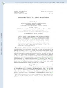
been able to come up with a closed expression for w (though one might exist). The function w vanishes at (1/2, 1/2) and does not contribute to the number of particles fluctuations. Figure (1) shows a two-dimensional plot of w which reveals that w(x, y) conveys anticorrelations for x, y in the vicinity of the reservoir with the highest density, while positive correlations develop close to the reservoir imposing the lowest density. The function w stands for the deviation of the long-range component of the density correlation function with respect to the pair interaction case (whether at small ε as in (52), or at ε → ∞ as computed by Spohn [16]). It is worth stressing that, to our knowledge, no microscopic model had, up to now, shown such strong deviations. The fluctuations of the total number of particles now read 2 2 ∆N 2 = ∆Nloc. eq. − 2Lε(ζ0 − ζ1 ) (ζ0 + ζ1 )

(60)

2 where ∆Nloc. eq. denotes the fluctuations of a systems in local thermal equilibrium with the same fugacity profile (such as the ZRP). In the present case the third cumulant is of order ε as well, and it has the formal expression and that

W (3) (x1 , x2 , x3 ) = −6εζ(x1 )3 δ(L(x1 − x2 ))δ(L(x2 − x3 )) Z 6ε − dτ dz(ζ0 (1 − z) + ζ1 z)G(x1 , z; τ )G(x2 , z; τ )G(x3 , z; τ ) L 16

(61)

w(x, y)

0.05

1 0.8

0 -0.05 0

0.6 0.4

0.2 0.4

x

y

0.2

0.6 0.8 10

Figure 1: Plot of w(x, y) [see eq.(59)] as a function of x, y ∈ [0, 1]. (3)

Denoting by WNE the function appearing in the second line of the r.h.s. of Eq. (61) allows to write the effective free energy in the form  Z 1  n 3 F [n(x)] = dx ρ + ερ − n + n ln + εn(n − 1)(n − 2) ρ + 3ερ3 0     Z n(x) 1 1 n(y) (2) dxdy − − 1 WNE (x, y) −1 2 0 ρ(x) ρ(y)     Z 1 1 n(x) n(y) n(z) (3) dxdydz − −1 −1 − 1 WNE (x, y, z) 3! 0 ρ(x) ρ(y) ρ(z) (62) As one can see, the triplet repulsion generates not only two-body long ranged repulsive interactions, but also three body interactions, repulsive as well. This establishes a correspondence between the microscopics (the precise form of h(n)) and the effective interactions generated by the boundary drive.

5.4 Competing interactions Suppose we now focus on a local interaction energy of the form h(n) = ε [−n(n − 1) + λn(n − 1)(n − 2)] , λ > 0 17

(63)

where the first term on the r.h.s., which favors pair condensation, is competing with the second term on the r.h.s. which assigns a relative energy cost λ to the piling up of three or more particles. To first order in ε the density correlation function is merely a linear combination of that obtained for the pair and triplet interactions, namely h i ε (2) 2 C (x < y) = (ζ0 − ζ1 ) (1 − 12λ(ζ0 + ζ1 ))x(1 − y) + 12λ(ζ0 − ζ1 )w(x, y) L (64) We can clearly see that, at sufficiently low densities, positive correlations develop, thus providing a microscopic counterexample to the general belief that the driving of a current builds up anticorrelations (note, however, that Spohn [16] had left this possibility a priori open).

6 Integrated current distribution Let Q(t) be the net number of particles which have jumped from the left reservoir into the system over the time interval [0, t] (counted positively for an actual jump from the reservoir into the system, and negatively for a jump out of the system to the reservoir). The physical motivations for studying the properties of Q are detailed by Lebowitz and Spohn [17] who showed that this quantity, defined for a Markov process (our boundary driven lattice gas with stochastic dynamics) plays a role analogous to the phase space contraction rate for dynamical systems (and for which Gallavotti and Cohen [18] proved their fluctuation theorem). Below, we shall concerned with the calculation of the distribution of Q(t).

6.1 Free particles Following the procedure described in [2, 6], we construct a master equation for P ({ni}, Q, t), the probability that the system is in state {ni } and with Q(t) = Q by explicitly separating those moves in phase space that increase Q by one, decrease it by one, or leave it unchanged. Introducing a state vector |ψ(Q, t)i = P P ({n i }, Q, t)|{ni }i, we are left with an evolution equation of the form {ni } d|ψ(Q, t)i ˆ1 + H ˆ −1 + H ˆ 0 )|ψ(Q, t)i = −(H dt

18

(65)

ˆ ± 1 increase/decrease Q by one, and where H ˆ 0 leave Q where the operators H unchanged. We are interested in the distribution function of Q(t) in the steady state, over large time intervals, p(Q, t) = hp|ψ(Q, t)i

(66)

or, more conveniently, its generating function, namely, pˆ(z, t) =

+∞ X

z Q p(Q, t)

(67)

Q=−∞

It turns out that the generating function can conveniently be expressed in terms of a path-integral Z Dˆ ai Dai e−S0,z [ˆa,a]

pˆ(z, t) =

(68)

where, for noninteracting particles Z t hX  X X S0,z [ˆ a, a] = − ai (t) + dτ a ˆi ∂τ ai + D (ˆ ai − a ˆj )ai 0

i

i

j

+ α(1 − zˆ a0 ) + γ(ˆ a0 − z −1 )a0 i + δ(1 − a ˆL ) + β(ˆ aL − 1)aL

(69)

The action S0,z does not describe a stochastic process (unless z = 1 for which it reduces to S0 ). However, it may be readily seen that Rt

pˆ(z, t) = he

0

dt(α(z−1)−γ(1−z −1 )a0 (t))

iz

(70)

where the brackets h..iz now denote an average with respect to the process governed by S0 in which α is formally replaced with αz. Using that a0 (t), for free particles, is a nonfluctuating field with expression taken from (21) by changing α into αz, zζ0 − ζ1 a0 (t) = ζ0 z − [1 − ε(4ζ0 z + ζ1 )] (71) γL we find that, in the long time limit, 1 z−1 ln pˆ(z, t) = µ(z) = (ζ0 z − ζ1 ) t→∞ t L z lim

19

(72)

It is a posteriori clear why subleading finite size corrections had to be kept all along. The function µ(z) is the generating function for the cumulants of Q. It is worth commenting on two remarkable, yet expected, properties of µ(ζ0 , ζ1, z). Namely, if we exchange the roles of the reservoirs, the distribution of Q is turned into that of −Q, hence µ(ζ0 , ζ1 , z) = µ(ζ1 , ζ0 , z −1 )

(73)

But it also satisfies the Gallavotti–Cohen property (see [17, 6] for a readable proof), namely ζ1 µ(ζ0 , ζ1 , z) = µ(ζ0 , ζ1 , ) (74) ζ0 z which is best known when rephrased as follows. Let π(Q) be the large deviation function related to p(Q, t): ln p(Q, t) t→∞ t

π(Q) = lim

(75)

Besides, π(Q) appears as the Legendre transform of µ(z) with respect to ln z:

hence

π(Q) = maxz {µ(ζ0, ζ1 , z) − ln zQ}

(76)

p(Q, t) ζ0 1 ln = π(Q) − π(−Q) = ln Q t→∞ t p(−Q, t) ζ1

(77)

lim

Of course this can a posteriori be verified on the explicit expression of π(Q): r Q Q2 ζ0 ζ1 q π(Q) = + + ζ0 ζ1 + 2 2 4 Q + Q4 + ζ0 ζ1 2  q 2 (78) Q Q + ζ ζ + 0 1 4 2  − (ζ0 + ζ1 ) − Q ln  ζ0

which is plotted on Fig. (2). The Gallavotti-Cohen theorem was shown [19, 17] to hold under quite general conditions for nonequilibrium steady-states resulting from Markovian dynamics and we shall further comment upon it in subsection 6.5.

20

π(Q) Q -2

2

4

6

-2 -4 -6 -8

Figure 2: Plot of π(Q) in eq.(78) for free particles with ρ0 = 1 ≫ ρ1 . Note the strong asymmetry of π.

6.2 Short Range Process with pair repulsion We now repeat the strategy outlined in the previous paragraph, but for the interacting case, with the short range process dynamics. We split the evolution operator ˆ ε into three pieces, each describing moves that increase, decrease of leave Q H unchanged. Then we pass to a path integral in terms of which we find Z pˆ(z, t) = Dˆ ai Dai e−Sε,z [ˆa,a] (79)

Having found Sε,z we bring the calculation of pˆ to that of a given observable with respect to the original stochastic process in which α is replaced with αz:  Z t h i −1 pˆ(z, t) = hexp − dt α(1 − z)(1 − εˆ a0 a0 ) + γ(1 − z )a0 (1 + εˆ a0 a0 ) iz 0

(80)

In order to evaluate the latter expectation value to leading order in ε we rely on a cumulant expansion. Introducing the variable ω(ζ0, ζ1 , z) = we find that

 z−1 (ζ0 − εζ02)z − (ζ1 − εζ12) − ε(z − 1)ζ0 ζ1 z ε Lµ = ω − ω 2 3 21

(81) (82)

It is remarkable that the intermediate variable ω itself satisfies the two invariance properties that µ is known to fulfill. Namely, the function ω(ρ0 , ρ1 , z) verifies the left-right symmetry ω(ζ0, ζ1 , z) = ω(ζ1, ζ0 , z −1 ) (83) and the Gallavotti–Cohen property ω(ζ0, ζ1 , z) = ω(ζ0 , ζ1,

ζ1 ) ζ0 z

(84)

That ω verifies (73,74) implies directly that µ possesses the same invariance properties, as already identified in the SEP [6]. One invariance property that our result does not possess, in constrast to [6], is the particle–hole symmetry. The effective small parameter of the expansion is ερ, where ρ is the typical density, hence our small ε expansion is seen to coincide with a low density expansion of the exact result obtained at ε → ∞ by [6],

with

1 8 Lµ = ω − ω 2 + ω 3 + O(ω 4 ) 3 45

(85)

  ζ0 ζ1 ζ0 ζ1 z−1 z− − (z − 1) ω= z 1 + ζ0 1 + ζ1 1 + ζ0 1 + ζ1

(86)

A natural question that arises next is how universal the result obtained in the exact calculation [6] is? How sensitive is it to varying the microscopic interactions. In order to sort out this issue we have performed a similar analysis for repulsive triplet interactions, with short range dynamics.

6.3 Short Range Process with triplet repulsion In the same spirit as in the previous paragraph, we express the generating function pˆ(z) as the expectation value of an exponential observable with respect to the lattice gas measure in which α is replaced with αz. We rely again on a cumulant expansion, and after a rather tedious calculation, we arrive at the following results. We now define the auxiliary variable ω by ω(ζ0, ζ1 , z) =

 z−1 (ζ0 − εζ03)z − (ζ1 − εζ13) − ε(z − 1)ζ0 ζ1 (ζ0 + ζ1 ) z  (87) εz−1 × 1− (ζ0 z − ζ1 )(ζ0 + ζ1 ) 2 z 22

which also obeys (73,74). We find that Lµ = ω −

ε 3 ω + O(ε2 ) 10

(88)

This expression unambiguously points at a different distribution function for the integrated current. It further allows to connect the microscopics –the triplet repulsion– with the final form of µ. A p-body interaction would yield a first correction to µ of the form ω p . Unfortunately we have not been able to come by a physical interpretation for the intermediate quantity ω.

6.4 Zero Range Process with pair repulsion Finally we examine the case of the zero range process with pair repulsion, for which we know that the steady state distribution follows local equilibrium. It is then sufficient to start from the equilibrium expression for the free process in which one has subsituted the current with its appropriate expression. It is not hard to see, through a direct evaluation, that (ζ0 − 2εζ02) − (ζ1 − 2εζ12) ρ0 − ρ1 hQi = α − γhn0 e2ε(n0 −1) i = ≃ t L L

(89)

which leads us to Lµ(ζ0 , ζ1, z) =

 z−1 (ζ0 − 2εζ02)z − (ζ1 − 2εζ12) z

(90)

This form is identical to that predicted by Bodineau and Derrida [12]) for zero range processes. The Gallavotti-Cohen relation, in our particular case, now takes the form ζ0 − 2εζ02 1 ) µ(ζ0 , ζ1 , z) = µ(ζ0, ζ1 , ζ1 − 2εζ12 z

(91)

It is remarkable that at equilibrium, that is for ρ0 = ρ1 , the current fluctuations hQ2 i is the same for the ZRP and the SRP, while higher order cumulants (that is the whole distribution) are different.

6.5 Illustration of the additivity principle To conlude this section, we would like to illustrate how our explicit results fit into the general framework provided by Bodineau and Derrida [12]. In particular, 23

they have deduced, from a postulated additivity principle, a general expression for the integrated current distribution, from the sole knowledge of hQi(ρ0 , ρ1 ) and hQ2 ic (ρ0 , ρ1 ). One of the consequences of their findings is a direct computation of the analog, in the Gallavotti-Cohen theorem, of the ”entropy production rate” (as formally defined by Lebowitz and Spohn [17]) in these driven stochastic lattice gases. Defining, as in [12], D(ρ) = they have shown that

1 ∂ hQ2 ic (ρ, ρ) hQi(ρ0 , ρ) , σ(ρ) = t ∂ρ0 t ρ0 =ρ  Z µ(z) = µ 2

ρ0

ρ1

D(ρ) 1 dρ σ(ρ) z



(92)

(93)

To leading order in ε, it is straighforward to see from (90) that, for the Zero Range Process, D(ρ) = 1, σ(ρ) = 2ρ (94) For the short range process, for pair interaction: D(ρ) = 1 + 2ερ, σ(ρ) = 2ρ for triplet interaction: D(ρ) = 1 + 6ερ2 , σ(ρ) = 2ρ

(95)

thus leading, in both cases, to µ(z) = µ(

ζ0 ) ζ1 z

(96)

Hence formula (93) is in perfect agreement with our explicit computations, not only for zero range processes, but also for the non trivial short range processes with pair or triplet repulsion.

7 Final remarks We have shown on specific examples that driving a system out of equilibrium magnifies the differences in the underlying microscopic dynamics. Not only the density profiles are different, but some dynamical rules lead the system to a state of local equilibrium, while others let it develop long range effective interactions. In all cases, however, our explicit results for the integrated current distribution 24

provide support for the postulated additivity principle of Bodineau and Derrida [12]. We should emphasize that the above results have been worked out by setting up a formalism, based on path integrals, which provides an alternative both to exact solutions and to the fluctuating hydrodynamics approach. The path integral formalism fills a gap in the sense that it allows us to go directly from a microscopic formulation to macroscopic properties and, furthermore, it allows formulating approximate approaches in nonequilibrium settings. Most of our results rely on a high temperature or virial like expansion, thus providing a intuitive parallel to the standard techniques of equilibrium statistical mechanics. We believe that several lines could now be explored. First, the present toolbox allows us to investigate the effect of additional space dimensions at little extra formal cost (even though calculations will undoubtedly be more involved). This would help to clearly isolate those feature which are characteristic of onedimensional systems from those that generalize to more realistic ones. An interesting problem arising in higher dimension is the interplay between longitudinal and transverse current fluctuations. Second, most of the quantities studied in the present work are time-independent, but the present toolbox makes possible the sudies of time-dependent quantities such as the time-dependent profile or effective free energy. Third, a natural extension of our formalism would consist of establishing nonperturbative results in ε. Much in the same way as in liquid state theory, infinite families of appropriately chosen Mayer diagrams can be summed up, and one could investigate which types of Feynman diagrams will contribute in building up the strongly nonlocal nature of the free energy functional found in [1]. Finally, extending our results for more complex geometries with more than two particle reservoirs, as suggested in [12] or done in [20], should allow us to identify the universal emerging features and to bring the theory closer to experiments. Ackownledgments. This research has been partially supported by the Hungarian Academy of Sciences (Grant No. OTKA T043734). The authors would like to thank Gunter Sch¨utz, Henk Hilhorst, Emmanuel Trizac and Alain Barrat for useful discussions, and further acknowledge Bernard Derrida for numerous useful suggestions.

25

References [1] B. Derrida, J. L. Lebowitz and E. R. Speer, Phys. Rev. Lett. 87, 150601 (2001) [cond-mat/0105110], Free Energy Functional for Nonequilibrium Systems: An Exactly Solvable Case. [2] B. Derrida and J. L. Lebowitz, Phys. Rev. Lett. 80, 209 (1998) [cond-mat/9809044], Exact Large Deviation Function in the Asymmetric Exclusion Process. [3] B. Derrida, J. L. Lebowitz and E. R. Speer J. Stat Phys. 107, 599 (2002) [cond-mat/0109346], Large Deviation of the Density Profile in the Steady State of the Open Symmetric Simple Exclusion Process. [4] B. Derrida, J. L. Lebowitz and E. R. Speer, J. Stat. Phys. 110, 775 (2003) [cond-mat/0205353], Exact Large Deviation Functional of a Stationary Open Driven Diffusive System: The Asymmetric Exclusion Process. [5] B. Derrida and C. Enaud, J. Stat. Phys. 114, 537 (2004), [cond-mat/0307023], Large deviation functional of the weakly asymmetric exclusion process. [6] B. Derrida, B, Douc¸ot and P.-E. Roche, J. Stat. Phys. 115, 713 (2004), [cond-mat/0310453], Current fluctuations in the one dimensional symmetric exclusion process with open boundaries. [7] L. Bertini, A. De Sole, D. Gabrielli, G. Jona-Lasinio and C. Landim, Phys. Rev. Lett. 87, 040601 (2001) [cond-mat/0104153], Fluctuations in Stationary non Equilibrium States. [8] L. Bertini, A. De Sole, D. Gabrielli, G. Jona-Lasinio, C. Landim, J. Stat. Phys. 107, 635 (2002) [cond-mat/0108040], Macroscopic fluctuation theory for stationary non equilibrium states. [9] L. Bertini, A. De Sole, D. Gabrielli, G. Jona-Lasinio and C. Landim, Math. Phys. Anal. Geom. 6, 231 (2003) [cond-mat/0307280], Large deviations for the boundary driven symmetric simple exclusion process. [10] F. Spitzer, Adv. Math. 5, 246 (1970), Interaction of Markov processes. [11] C. Cocozza-Thivent, Z. Warhsch. Verw. Gebiete, 70, 509 (1995), Processus des misanthropes. 26

[12] T. Bodineau and B. Derrida, Phys. Rev. Lett. in press [cond-mat/0402305], Current fluctuations in nonequilibrium diffusive systems: an additivity principle. [13] For references and a review of recent developments in zero range processes see G. M. Sch¨utz, J. Phys. A 36, R339 (2003) [cond-mat/0308450], Critical phenomena and universal dynamics in one-dimensional driven diffusive systems with two species of particles. [14] D.C. Mattis and M.L. Glasser, Rev. Mod. Phys. 70, 979 (1998), The uses of quantum field theory in diffusion-limited reactions. [15] This was shown to us by G. Sch¨utz, private communication. [16] H. Spohn, J. Phys. A 16, 4275 (1983), Long range correlations for stochastic lattice gases in a nonequilibrium steady-state. [17] J.L. Lebowitz and H. Spohn, J. Stat. Phys. 95, 333 (1999) [cond-mat/9811220], A Gallavotti-Cohen Type Symmetry in the Large Deviation Functional for Stochastic Dynamics. [18] G. Gallavotti and E.G.D. Cohen, Phys. Rev. Lett. 74, 2694 (1995) [chao-dyn/9410007], Dynamical ensembles in nonequilibrium statistical mechanics. [19] J. Kurchan, J. Phys. A 31, 3719 (1998) [cond-mat/9709304], Fluctuation theorem for stochastic dynamics. [20] Ya.M. Blanter and M. B¨uttiker, Phys. Rev. B 56, 2127 (1997) [cond-mat/9702047], Shot noise current-current correlations in multiterminal diffusive conductors.

27