Large-eddy simulation of wind flows over complex ...

Ashvinkumar Chaudhari

LARGE-EDDY SIMULATION OF WIND FLOWS OVER COMPLEX TERRAINS FOR WIND ENERGY APPLICATIONS Thesis for the degree of Doctor of Science (Technology) to be presented with due permission for public examination and criticism in Auditorium 1303 at Lappeenranta University of Technology, Lappeenranta, Finland on the 5th of December, 2014, at 12:00.

Acta Universitatis Lappeenrantaensis 598

Supervisors

Professor, PhD Jari Hämäläinen Faculty of Technology Centre of Computational Engineering and Integrated Design (CEID) Department of Mathematics and Physics Lappeenranta University of Technology Finland Docent, D.Sc. Antti Hellsten Atmospheric Dispersion Modelling Atmospheric Composition Research Finnish Meteorological Institute (FMI) P.O. Box 503, FI-00101 Helsinki Finland

Reviewers

Professor, PhD Bert Blocken Department of the Built Environment Eindhoven University of Technology The Netherlands PhD Catherine Gorle Center for Turbulence Research Stanford University USA

Opponent

Professor, PhD Bert Blocken Department of the Built Environment Eindhoven University of Technology The Netherlands

ISBN 978-952-265-674-2 ISBN 978-952-265-675-9 (PDF) ISSN-L 1456-4491 ISSN 1456-4491 Lappeenrannan teknillinen yliopisto Yliopistopaino 2014

Abstract Ashvinkumar Chaudhari LARGE-EDDY SIMULATION OF WIND FLOWS OVER COMPLEX TERRAINS FOR WIND ENERGY APPLICATIONS Lappeenranta, 2014 110 p. Acta Universitatis Lappeenrantaensis 598 Diss. Lappeenranta University of Technology ISBN 978-952-265-674-2, ISBN 978-952-265-675-9 (PDF), ISSN-L 1456-4491, ISSN 1456-4491 Wind energy has obtained outstanding expectations due to risks of global warming and nuclear energy production plant accidents. Nowadays, wind farms are often constructed in areas of complex terrain. A potential wind farm location must have the site thoroughly surveyed and the wind climatology analyzed before installing any hardware. Therefore, modeling of Atmospheric Boundary Layer (ABL) flows over complex terrains containing, e.g. hills, forest, and lakes is of great interest in wind energy applications, as it can help in locating and optimizing the wind farms. Numerical modeling of wind flows using Computational Fluid Dynamics (CFD) has become a popular technique during the last few decades. Due to the inherent flow variability and large-scale unsteadiness typical in ABL flows in general and especially over complex terrains, the flow can be difficult to be predicted accurately enough by using the Reynolds-Averaged Navier-Stokes equations (RANS). LargeEddy Simulation (LES) resolves the largest and thus most important turbulent eddies and models only the small-scale motions which are more universal than the large eddies and thus easier to model. Therefore, LES is expected to be more suitable for this kind of simulations although it is computationally more expensive than the RANS approach. With the fast development of computers and open-source CFD software during the recent years, the application of LES toward atmospheric flow is becoming increasingly common nowadays. The aim of the work is to simulate atmospheric flows over realistic and complex terrains by means of LES. Evaluation of potential in-land wind park locations will be the main application for these simulations. Development of the LES methodology to simulate the atmospheric flows over realistic terrains is reported in the thesis. The work also aims at validating the LES methodology at a real scale. In the thesis, LES are carried out for flow problems ranging from basic channel flows to real atmospheric flows over one of the most recent real-life complex terrain problems, the Bolund hill. R All the simulations reported in the thesis are carried out using a new OpenFOAM -based LES solver. The solver uses the 4th order time-accurate Runge-Kutta scheme and a fractional step method. Moreover, development of the LES methodology includes special attention to two boundary conditions: the upstream (inflow) and wall boundary conditions. The upstream boundary condition is generated by using the so-called recycling technique,

in which the instantaneous flow properties are sampled on a plane downstream of the inlet and mapped back to the inlet at each time step. This technique develops the upstream boundary-layer flow together with the inflow turbulence without using any precursor simulation and thus within a single computational domain. The roughness of the terrain surface R is modeled by implementing a new wall function into OpenFOAM during the thesis work. Both, the recycling method and the newly implemented wall function, are validated for the channel flows at relatively high Reynolds number before applying them to the atmospheric flow applications. After validating the LES model over simple flows, the simulations are carried out for atmospheric boundary-layer flows over two types of hills: first, two-dimensional wind-tunnel hill profiles and second, the Bolund hill located in Roskilde Fjord, Denmark. For the twodimensional wind-tunnel hills, the study focuses on the overall flow behavior as a function of the hill slope. Moreover, the simulations are repeated using another wall function suitR able for smooth surfaces, which already existed in OpenFOAM , in order to study the sensitivity of the flow to the surface roughness in ABL flows. The simulated results obtained using the two wall functions are compared against the wind-tunnel measurements. It is shown that LES using the implemented wall function produces overall satisfactory results on the turbulent flow over the two-dimensional hills. The prediction of the flow separation and reattachment-length for the steeper hill is closer to the measurements than the other numerical studies reported in the past for the same hill geometry. The field measurement campaign performed over the Bolund hill provides the most recent field-experiment dataset for the mean flow and the turbulence properties. A number of research groups have simulated the wind flows over the Bolund hill. Due to the challenging features of the hill such as the almost vertical hill slope, it is considered as an ideal experimental test case for validating micro-scale CFD models for wind energy applications. In this work, the simulated results obtained for two wind directions are compared against the field measurements. It is shown that the present LES can reproduce the complex turbulent wind flow structures over a complicated terrain such as the Bolund hill. Especially, the present LES results show the best prediction of the turbulent kinetic energy with an average error of 24.1%, which is a 43% smaller than any other model results reported in the past for the Bolund case. Finally, the validated LES methodology is demonstrated to simulate the wind flow over the existing Muukko wind farm located in South-Eastern Finland. The simulation is carried out only for one wind direction and the results on the instantaneous and time-averaged wind speeds are briefly reported. The demonstration case is followed by discussions on the practical aspects of LES for the wind resource assessment over a realistic inland wind farm. Keywords: LES, Complex terrains, Atmospheric flows, Bolund hill, Boundary layer, LES upstream boundary condition, OpenFOAM UDC 621.311.245:533.6.011:004.942

Acknowledgments

The research work has been carried out in the Centre of Computational Engineering and Integrated Design (CEID) of Lappeenranta University of Technology (LUT) during years 2011-2014. The work presented here has been a part of the RENEWTECH project which was aimed for the development of wind power technology and business in Southern Finland from 2011-2013, and it was funded by the European Regional Development Fund (ERDF). A part of the funding was also received from Department of Mathematics and Physics and the CEID center in LUT. I highly appreciate all the financial supports. During the work, the high-performance computing resources were provided by CSC-IT Center for Science Ltd, Espoo, Finland. The research work presented in this thesis would have been impossible to accomplish without the support of CSC. Moreover, I would like to acknowledge the National Land Survey of Finland (NLS) for providing the terrain-elevation dataset for the wind-farm topography free of charge. Foremost, I would like to express my heartfelt gratitude to my supervisors Prof. Jari Hämäläinen and Dr. Antti Hellsten for all the scientific guidance and support they have provided throughout this entire research. I am very much grateful to both of you for giving me an opportunity to work in the fascinating area of atmospheric flow modelling using "LES" method. Next, I would like to express my sincere thanks to Prof. Heikki Haario and Prof. Tuomo Kauranne for their kind support and help especially in starting-up this study and also for their helpful discussion during the study. I am also most grateful to the reviewers of this thesis, Prof. Bert Blocken and Dr. Catherine Gorle. Your valuable feedback helped me greatly to improve and finalize this thesis. I would like to thank all co-authors of my publications as well as my collaborators during the research work. Especially, Dr. Ville Vuorinen from Aalto University, Dr. Boris Conan from École Centrale de Nantes (France), Dr. Gábor Janiga from University of Magdeburg (Germany), Dr. Federico Roman from University of Trieste (Italy) and M.Sc. Oxana Agafonova from LUT, I am thankful for your contribution and collaboration as well as for helpful discussions on the topic. I would also like to thank Esko Jarvinen from CSC for his technical help in running the simulations on super-computing environment. It is pleasure to thank many friends for their valuable help and support. My thanks go to my friends Zuned, Paritosh, Arjun, Naresh, Miika, Matylda, Piotr and Ville. I deeply appreciate your moral support during my entire stay in Lappeenranta. I would also like to thank all my co-workers from the CEID centre and the Mathematics department, fellow students, and other friends in Finland as well as in abroad. Last but not the least, I would like to express my deepest gratitude to my parents for their blessings during my education. I thank them for educating and supporting me in every stage of my life. I am very much grateful to my beloved wife, Bhavana for her love, and support. I believe that without your support this work would not have been in a proper shape.

Lappeenranta, November 2014 Ashvinkumar Chaudhari

C ONTENTS

Abstract Preface Contents List of publications and the author’s contribution Nomenclature 1 Introduction 15 1.1 Motivation . . . . . . . . . . . . . . . . . . . . . . . . . . . . . . . . . . . 15 1.2 Literature review . . . . . . . . . . . . . . . . . . . . . . . . . . . . . . . 17 1.3 Objectives and overview of the thesis . . . . . . . . . . . . . . . . . . . . . 18 2

3

LES methodology 2.1 Governing equations . . . . . . . . . . . . . . . . . . . . . . . . . . . . 2.2 Projection method . . . . . . . . . . . . . . . . . . . . . . . . . . . . . . 2.2.1 Helmholtz-Hodge decomposition . . . . . . . . . . . . . . . . . 2.2.2 Implementation of the projection method . . . . . . . . . . . . . 2.3 Sub-grid scale model . . . . . . . . . . . . . . . . . . . . . . . . . . . . 2.4 LES for channel flows . . . . . . . . . . . . . . . . . . . . . . . . . . . . 2.5 Wall-function model . . . . . . . . . . . . . . . . . . . . . . . . . . . . 2.5.1 Smooth wall function . . . . . . . . . . . . . . . . . . . . . . . . 2.5.2 Implementation and validation of new wall-function for a rough surface condition . . . . . . . . . . . . . . . . . . . . . . . . . . 2.6 Inflow boundary condition . . . . . . . . . . . . . . . . . . . . . . . . .

. 29 . 32

Flow over two-dimensional wind-tunnel hills 3.1 Background . . . . . . . . . . . . . . . . 3.2 Computational set-up . . . . . . . . . . . 3.2.1 Computational domain and grid . 3.2.2 Boundary conditions . . . . . . . 3.3 Results and discussion . . . . . . . . . . 3.3.1 Upstream boundary-layer flow . . 3.3.2 Flow over the hills . . . . . . . . 3.4 Conclusions . . . . . . . . . . . . . . . .

. . . . . . . .

. . . . . . . .

. . . . . . . .

. . . . . . . .

. . . . . . . .

. . . . . . . .

. . . . . . . .

. . . . . . . .

. . . . . . . .

. . . . . . . .

. . . . . . . .

. . . . . . . .

. . . . . . . .

. . . . . . . .

. . . . . . . .

. . . . . . . .

. . . . . . . .

. . . . . . . .

. . . . . . . .

21 21 22 22 22 23 25 27 27

39 39 42 42 45 45 45 46 60

4

5

6

LES for a realistic terrain: the Bolund hill 4.1 The Bolund experiment . . . . . . . . . 4.2 Simulation set-up . . . . . . . . . . . . 4.2.1 Computational domain and grid 4.2.2 Boundary conditions . . . . . . 4.3 Results and discussion . . . . . . . . . 4.4 Conclusions . . . . . . . . . . . . . . .

. . . . . .

. . . . . .

. . . . . .

. . . . . .

. . . . . .

. . . . . .

. . . . . .

. . . . . .

. . . . . .

. . . . . .

. . . . . .

. . . . . .

. . . . . .

. . . . . .

63 63 66 66 69 69 86

Towards practical applications 5.1 Muukko wind-park demonstration case . . . . . . . 5.1.1 Wind-farm geometry and simulation details 5.1.2 Grid resolution and boundary conditions . . 5.1.3 Results . . . . . . . . . . . . . . . . . . . 5.2 Further practical aspects . . . . . . . . . . . . . .

. . . . .

. . . . .

. . . . .

. . . . .

. . . . .

. . . . .

. . . . .

. . . . .

. . . . .

. . . . .

. . . . .

. . . . .

. . . . .

89 89 89 90 92 95

. . . . . .

. . . . . .

. . . . . .

. . . . . .

. . . . . .

Summary

99

Bibliography

103

L IST OF PUBLICATIONS AND THE AUTHOR ’ S CONTRIBUTION

This monograph contains material from the following papers. I

Chaudhari, A., Hellsten, A., Agafonova, O. and Hämäläinen, J. Large-Eddy Simulation of Boundary-Layer Flows over Two-Dimensional Hills. In: F. Magnus, G. Michael, M. Nicole (Eds.) Progress in Industrial Mathematics at ECMI 2012. Mathematics in Industry, 19, 211-218, 2014.

II Chaudhari, A., Ghaderi Masouleh, M., Janiga, G., Hämäläinen, J. and Hellsten, A. (2014) Large-Eddy Simulation of Atmospheric Flows over the Bolund Hill. In: Proceedings of 6th International Symposium on Computational Wind Engineering (CWE-2014), Hamburg, Germany III Chaudhari, A., Vuorinen,V., Agafonova, O., Hellsten, A. and Hämäläinen, J. (2014) Large-Eddy Simulation for Atmospheric Boundary Layer Flows over Complex Terrains with Applications in Wind Energy. In: Proceedings of the 11th World Congress on Computational Mechanics (WCCM XI), Barcelona, Spain IV

Agafonova, O., Koivuniemi, A., Chaudhari, A. and Hämäläinen, J. (2014) Limits of WAsP Modelling in Comparison with CFD for Wind Flow over TwoDimensional Hills. In: Proceedings of European Wind Energy Association conference (EWEA-2014), Barcelona, Spain

V

Agafonova, O., Koivuniemi, A., Conan, B., Chaudhari, A., Haario, H. and Hämäläinen, J. (2014) Numerical and Experimental Modelling of Wind Flows over Hills. In: Proceedings of 18th European Conference on Mathematics for Industry (ECMI-2014), Taormina, Italy

VI Vuorinen,V., Chaudhari, A., and Keskinen, J.-P. Large-Eddy Simulation in R Complex Hill Terrains Enabled by Compact Fractional Step OpenFOAM Solver. Advances in Engineering Software, 79(0), 70-80, 2015.

Submitted Scientific Journal Articles VII Chaudhari, A., Vuorinen,V., Agafonova, O., Hämäläinen, J. and Hellsten, A. Large-Eddy Simulations for Hill Terrains: Validation with Wind-Tunnel and Field Measurements. Submitted to Flow, Turbulence and combustion. VIII Conan, B., Chaudhari, A., Aubrun, S., van Beeck, J.P.A.J., Hämäläinen, J. and Hellsten, A. Experimental and Numerical Modelling of Flow over Complex Terrain: the Bolund Hill. Submitted to Boundary-Layer Meteorology.

A. Chaudhari is the principal author and investigator in Publications I, II, III and VII. The author carried out all the numerical simulations and wrote majority of the articles’ text. O. Agafonova was responsible for post-processing of the numerical results. Docent Antti Hellsten and Prof. Jari Hämäläinen were responsible for supervising the work. In Publications IV and V, A. Chaudhari is a co-author and was responsible for carrying out a part of the numerical simulations. He wrote respective part of the articles together with the principal author O. Agafonova. Moreover, A. Chaudhari was partially responsible in supervising the work of the principal author O. Agafonova. Publication VI is an outcome of a collaboration with V. Vuorinen from Combustion and Thermodynamics research group at the Aalto University School of Engineering, Espoo. R The principal author V. Vuorinen implemented new numerical flow solver into OpenFOAM . R

A. Chaudhari incorporated new wall-function boundary condition into OpenFOAM and carried out numerical simulation in order to validate the simulation methodology. Also, A. Chaudhari wrote a part of the manuscript together with the principal author. Publication VIII is also written in a collaboration with B. Conan from École Centrale de Nantes (France). In this publication, B. Conan performed wind-tunnel experiment for the Bolund flows, whereas author A. Chaudhari carried out numerical simulation for the same flow problem. A. Chaudhari also wrote respective part of the manuscript.

N OMENCLATURE

Abbreviations ABL CFD CFL CSP DES DNS ERCOFTAC EU EWEA FAC2 FB FVM GW GWEC IBM LES MAE MW NMSE NWP PDF PISO PV

Atmospheric Boundary Layer Computational Fluid Dynamics Courant-Friedrichs-Levy-number Concentrating Solar Power Detached-Eddy Simulation Direct Numerical Simulation European Research Community On Flow, Turbulence And Combustion European Union European Wind Energy Association Factor two Fractional Bias Finite Volume Method Giga Watt Global Wind Energy Council Immersed Boundary Method Large-Eddy Simulation Mean Absolute Error Mega Watt Normalized Mean Square Error Numerical Weather Prediction Probability Density Function Pressure-Implicit with Splitting of Operators Photo Voltaic

OpenFOAM RANS RK RMS SGS STL TKE WSS

Greek Letters δ ∆ ∆k ∆S ∆t ∆x, ∆y, ∆z κ µ µef f ν νsgs ρ τw τij

Open source Field Operation And Manipulation Reynolds-Averaged Navier-Stokes Runge-Kutta Root Mean Square Sub-Grid Scales STereoLithography Turbulent Kinetic Energy Wall Shear Stress

Boundary-Layer depth Cutoff length, filter width TKE increase Speed-up Time step Grid spacing in x, y, z-directions von Kármán constant Dynamic viscosity Effective dynamic viscosity Kinematic molecular viscosity Kinematic SGS viscosity Density Wall shear stress SGS stress tensor

Symbols a C k , C Cs d H k ks ksgs Lrcy Lx , Ly , Lz Nx , Ny , Nz p˜ Re Reτ ReH RS Rk S S˜ij t u˜i u0 uτ , u∗ , u∗0 U∞ U V x, y, z z0 zagl

Hill half-length Sub-Grid Scale model constants The Smagorinsky model constant Diameter (height) of the computational domain Hill height Turbulent kinetic energy Sand-grain roughness height Sub-grid scale turbulent kinetic energy Recycling length Length of computational domain in x, y, z-directions Number of computational cells in x, y, z-directions Resolved instantaneous pressure Reynolds number Frictional Reynolds number Reynolds number based on hill height Speed-up error TKE error Mean velocity magnitude Strain rate tensor Time Resolved instantaneous velocity Resolved velocity fluctuation Frictional velocity Free-stream velocity Resolved mean velocity Volume Cartesian coordinates, z is the vertical coordinate Roughness length Height above the ground level

C HAPTER I

Introduction

1.1

Motivation

The production of wind energy is of ever-increasing interest due to risks of global warming and nuclear energy production plant accidents. For more than a decade, wind energy has been the fastest growing energy technology worldwide, achieving an annual growth rate of over 30%. By the end of 2013, six countries had more than 10,000 MW installed wind power capacity including China (91,412 MW), the US (61,091 MW), Germany (34,250 MW), Spain (22,959 MW), India (20,150 MW) and the UK (10,531 MW) (GWEC, 2014). Annual wind power installations in the EU have increased steadily over the past 13 years from 12,887 MW (2%) in 2000 to 117,288 MW (13%) in 2013, representing an average annual growth rate of over 10% (EWEA, 2014). Figure 1.1 shows the contribution of different energy sources to the total power capacity in the EU for the year 2013. In Denmark, the wind power production in December 2013 accounted for more than 50% of the Danish electricity consumption for the whole month. The Danish wind power’s share of national electricity consumption rose to 33.2% (4,772 MW) in 2013 from 30.1% (4,162 MW) in 2012. And, the government together with the wind industry is working hard towards the goal of 50% wind power by the year 2020. The amount of installed wind power capacity in Finland is rather low compared to that of other European countries. In the end of 2011, wind power capacity in Finland was 197 MW which equals to only 0.5% share of country’s total electricity consumption, and however it has been growing slowly to 288 MW in 2012 and 448 MW by end of 2013. Finland has a national target to increase the share of renewable energy to 38% by 2020, in line with the obligation proposed for Finland by the EU Commission1 . Recently, several proposals and projects have been approved for the development of wind power technology in Finland. For example, the RENEWTECH project2 from 2011-2013 aimed for the development of wind power technology and business in South-East Finland. It is worth to mention that the present thesis is a part of the RENEWTECH project. Nowadays many wind farms (onshore) are being constructed in areas with complex topographies containing hills, ridges, forests and mountains with an intention to reach higher 1 2

http://www.tuulivoimayhdistys.fi/tariff http://www.renewtech.fi/

15

16

1. Introduction

Figure 1.1: EU power capacity mix in MW during year 2013 (EWEA, 2014).

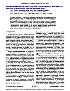
wind speeds. For example, European Wind Energy Association (EWEA) has reported that out of the 117.3 GW wind power installed in the EU by the end of 2013, around 110.7 GW (94%) wind farm installation is onshore and only 6.6 GW is offshore (EWEA, 2014). The advantages of onshore wind farms are that they tend to be cheaper to install and provide local, distributed generation of power. Although establishing a wind turbine over a hill or a mountainous area has its own advantages, it proposes specific difficulties such as a considerable surge in structural loads on the wind turbine blades due to the inherent flow variability and large-scale unsteadiness that is characteristic for the Atmospheric Boundary Layer (ABL). When considering flow over complex terrain these effects are reinforced and flow separation can occur. The ABL is the lowest part of the Earth’s atmosphere with a thickness ranging from a few tens of meters in stable wind conditions to approximately two kilometers depending on weather conditions. It is directly influenced by the local orography and surface roughness over which the wind flows. Figure 1.2 gives a general overview of a typical ABL flow over complex terrains. In such conditions, the evaluation of the wind resource becomes more and more challenging. The output power from a wind turbine is directly proportional to the cube of the wind speed such that a small wind speed-up corresponds to a very large power increase (Troen and Lundtang Petersen, 1989). Moreover, the height of the maximum wind speed-up is also important for engineers in order to estimate the wind loads on structures that are located on the hill top, such as antennas and power transmission towers (Paiva et al., 2009). The accurate evaluation of the wind speed is then of utmost importance for the estimation of the profitability of a wind farm. In addition to the wind speed, the turbulence level is equally important for the choice of a turbine. Therefore, the modeling of wind flows over complex terrains is of great interest in wind energy applications, as it can help in locating and optimizing the wind farms.

1.2 Literature review

17

Figure 1.2: Schematic picture of Atmospheric Boundary Layer (ABL). Courtesy of Marcelo Chamecki.

1.2

Literature review

A field measurement campaign is the only way to measure the wind resource as it accounts for all environmental parameters and weather fluctuations. However, it must be performed over years to get reliable statistics. In practice, such measurement campaigns are long and costly to be carried out for each new wind farm. In the literature, several field experiments have been performed in the past to study wind flows over the real topographies like the Black mountain (Bradley, 1980), the Ailsa Craig island, the Blashaval hill (Mason and King, 1985), the Askervein hill (Taylor and Teunissen, 1987), the Kettles hill (Salmon et al., 1988), and recently the Bolund hill (Berg et al., 2011). Among those, the Askervein hill project is the most well-known field campaign and has been the standard case to validate numerical codes and to evaluate turbulence models. Although, field campaigns are the only way to get real data, the measurements are often limited to point measurements at a limited number of locations that may not be sufficient to characterize the wind flow on a wind farm site or to optimize wind turbine positions. To complement field measurements, several numerical and experimental models have been developed over the years for predicting wind resources. These approaches can provide a valuable set of data where no field measurements are available. However the modeling of the atmosphere has to be validated with field measurements. Numerical modeling of wind flow using Computational Fluid Dynamics (CFD) has become a popular technique. So far in CFD, a wide range of diverse numerical methods have been introduced and utilized to simulate wind flow over complex terrains. The models are ranging from very simple linear models to non-linear models such as Reynolds-averaged Navier-stokes (RANS), and even more advanced models including Large-Eddy Simulation (LES) and Detached-Eddy Simulation (DES). The linearized flow models can predict the wind resource reasonably over sufficiently smooth terrain where the flow is always attached, but they cannot take into account flow separation. Thus, they are mainly used in large area applications to derive wind atlases. The RANS approach using two-equation turbulence models has been widely used for simulating atmospheric flows over the isolated hills or ridges (Apsley and Castro, 1997; Castro and Apsley, 1997; Kim et al., 1997; Griffiths and Middleton, 2010; Finardi et al., 1993; Kim et al., 2001; Loureiro et al., 2008; Snyder et al., 1991; Ying and Canuto, 1997; Agafonova et al., 2014). The approach has been successively extended towards wind prediction over complex terrains such as the Askervein hill located in Scotland by Castro et al. (2003),

1. Introduction

18

Kim et al. (2000), Paiva et al. (2009), Undheim et al. (2006) and Moreira et al. (2012), the Serra das Meadas mountainous located in North of Portugal by Maurizi et al. (1998), the Blashaval hill by El Kasmi and Masson (2010), and the Bolund hill located in the Denmark by Bechmann et al. (2011) and Prospathopoulos et al. (2012). Today, the RANS approach is considered as a good compromise between the accuracy of the results and the computational cost (Prospathopoulos et al., 2012). Although RANS models perform reasonably well for the mean wind prediction over such topographies, they may not perform well in the flows containing complex phenomena such as strong streamline curvature, acceleration, deceleration and separation, as they are calibrated in simple flows. Furthermore, the prediction of the turbulence properties will affect simulation results for the loads on wind turbines, the dispersion of pollutants, and weather prediction (Silva Lopes et al., 2007), and it is known that RANS-based models have limited accuracy for the turbulent quantities. To overcome these issues, advanced models such as LES, DES, or hybrid LES/RANS are encouraged to be applied to such atmospheric simulations. Since LES resolves the large turbulent motions of the flow and models only the smaller scales, it is therefore able to capture the important unsteadiness of the flow. Although the resources required by LES are much larger than those required by RANS simulation, the use of LES towards atmospheric flow simulation is becoming increasingly common nowadays due to the rapid evolution of the computer technology. Using LES, many researchers have studied wind flows over the two-dimensional hill (2D) shaped obstacles mostly at laboratory scale (Allen and Brown, 2002; Brown et al., 2001; Cao et al., 2012; Chaudhari et al., 2014b,c; Gong et al., 1996; Hattori et al., 2013; Henn and Sykes, 1999; Tamura et al., 2007; Wan et al., 2007; Wan and Porté-Agel, 2011). But the application of LES over a real topography is less common due to unique numerical challenges, such as a complex topography itself, the use of realistic upstream boundary conditions, inhomogeneous ground-roughness, resolving the near-wall turbulence structures, extremely high Reynolds number flow, etc. Nevertheless, some studies have been reported mostly for simulating the flow over the Askervein hill (Bechmann, 2006; Bechmann and Sørensen, 2010; Silva Lopes et al., 2007; Chow and Street, 2009; Golaz et al., 2009). Silva Lopes et al. (2007) studied the grid resolution and effect of flow separation by using a hybrid RANS/LES model. Reinert et al. (2007) proposed a new LES model for simulating air flow above highly complex terrain. Bechmann and Sørensen (2010) proposed a hybrid RANS/LES method to simulate atmospheric flows over complex terrains. However, they reported that RANS and new hybrid models give different results in the wake region. In a more recent work by Diebold et al. (2013), LES is employed over the Bolund hill by utilizing the Immersed Boundary Method (IBM), that is, a numerical technique to incorporate terrain topography into CFD simulation with rectangular grids. However, more research and investigations are necessary to have a better vision of LES modeling over complicated terrains.

1.3

Objectives and overview of the thesis

The central goal of the thesis is to simulate atmospheric flows and to predict wind resources over realistic terrains. Evaluation of potential in-land wind park locations will be the main application for the simulations. Due to inherent flow variability and large-scale unsteadiness typical in the ABL in general and especially over complex terrains, the accuracy of

1.3 Objectives and overview of the thesis

19

RANS predictions, which represent all these effect by a turbulence model, is compromised. Therefore, LES is expected to be more suitable for this kind of simulations although it is computationally more expensive than the RANS approach. The objective here is to develop a LES methodology to be employed for simulating ABL flows over realistic and complex terrains. The work also aims at validating the LES methodology with the wind-tunnel measurements at laboratory scale as well as with the real field experimental measurements at full scale. Thus, the validated LES methodology can be employed for predicting the wind resources over other real terrains to support field measurements. Although the present thesis deals with the flow over complex terrains, the modeling of forest canopy is beyond the scope of the present work as it requires special attention. In order to achieve the goal, the intermediate steps are: R • Implementation of LES solver into the OpenFOAM code, and its preliminary validation for fully-developed channel flows at the frictional Reynolds numbers Reτ = 180 and Reτ = 395.

• To employ the LES model for simulating boundary-layer flows in channels at high Reynolds numbers and with coarse grid resolutions, typical for the ABL, using the existing wall-function boundary condition. • Development and validation of the inflow (upstream) and rough-wall function boundary conditions to be employed for ABL flow simulations over complex terrains. • To investigate the turbulent boundary-layer flows over idealized hills. Parametric study of the two-dimensional hill shaped profiles with two different slopes. Simulation using two surface conditions: smooth and rough. LES model validation using the wind-tunnel measurements. • To extend the LES methodology to simulate the local atmospheric flow over a realworld complex hill terrain: the Bolund hill. Validation of the results with the field measurements at full scale. • To demonstrate the validated LES methodology to simulate the wind resource assessment for a practical case: a real wind farm located in South-East Finland. The thesis is organized as follows. The introduction is followed by Chapter 2 which deals with the development of the LES methodology. It describes the governing equations of the LES modeling. The validation of the LES model for the boundary-layer flows in channel with smooth surface at different frictional Reynolds numbers is presented. Moreover, the theoretical implementation of the rough-wall function boundary condition (Section 2.5.2) followed by the development of the upstream boundary condition (Section 2.6) is discussed. Both boundary-condition methods are validated for the channel flows at high Reynolds numbers. Chapter 3 focuses on the validation of the LES methodology for the boundary-layer flows over the idealized hills at the wind-tunnel scale. A LES methodology described in Chapter 2 is employed to simulate the neutral ABL flow over the two-dimensional hill profiles or ridges with two different slopes. Moreover, both hill shapes are studied for the smooth and

20

1. Introduction

rough surface conditions. The chapter discusses the comparison between the LES results from both surface conditions and the wind-tunnel measurement. Based on the discussions some conclusions are drawn. In Chapter 4, the LES model validated over the two-dimensional wind-tunnel hill profiles is further validated over a real-life complex terrain problem called the Bolund hill. Here, LES calculations are carried out to investigate neutrally stratified atmospheric flow over the complicated Bolund hill for two different wind directions: 270◦ and 239◦ . The LES results for both wind directions are compared with the field measurements. The validation of the results is discussed and conclusions are drawn. Chapter 5 demonstrates the validated LES methodology for simulating the wind flow over the Muukko wind farm located in South-Eastern Finland. In this chapter, first the demonstration case is presented in Section 5.1 and it is followed by a further discussion on the practical aspects of LES for the wind resource assessment over a realistic inland wind farm (Section 5.2). The chapter also discusses future prospects. Finally, the last chapter summarizes the thesis.

C HAPTER II

LES methodology

2.1

Governing equations

Larger turbulent eddies which are the most energetic ones and responsible for the majority of turbulent transport are resolved directly in a computational grid in LES, whereas eddies smaller than the grid size are assumed to be more isotropic and are modeled using a SubGrid-Scale (SGS) model. The governing equations for LES are obtained by filtering the original continuity and Navier-Stokes equations. Thus, the filtered governing equations for incompressible flow can be written as ∂ u˜i =0 ∂xi ∂ ∂ ∂ (u˜i ) + (u˜i u˜j ) = ν ∂t ∂xj ∂xj

(2.1)



∂ u˜i ∂xj

 −

1 ∂ p˜ ∂τij − ρ ∂xi ∂xj

(2.2)

where u˜i and p˜ are the grid-filtered values of the velocity and the pressure, respectively, ν is the kinematic viscosity, ρ is the fluid density, and τij is the sub-grid scale stress defined as follows τij = ug ˜i u˜j . i uj − u

(2.3)

R In this thesis, the finite-volume method based open-source C++ code OpenFOAM (OpenCFD, R 2013) is employed to solve the governing equations. The greatest benefits of OpenFOAM have been (1) the utilization of license free CFD simulations, (2) capability to parallel computing, and (3) the flexibility of the high-level code syntax which provides an opportunity R to implement new flow solvers using the already existing C++ OpenFOAM libraries.

All the simulations reported in the thesis are carried out using new LES solver, called R here rk4ProjectionFoam, recently implemented into OpenFOAM (Vuorinen et al., 2015). The solver is based on the fourth order Runge-Kutta (RK4) time integration, and the R projection method for pressure-velocity coupling. It was first incorporated into OpenFOAM 21

2. LES methodology

22

by Vuorinen et al. (2014) and further extended for the atmospheric flows during the thesis work (Vuorinen et al., 2015). The solver rk4ProjectionFoam is computationally efficient, and typically numerically less dissipative than the standard pisoFoam solver of R OpenFOAM (Vuorinen et al., 2014). In the following, the implementation of the solver is discussed.

2.2

Projection method

2.2.1 Helmholtz-Hodge decomposition The projection method links the pressure-velocity coupling to the well known HelmholtzHodge (HH) decomposition (Canuto et al., 2007; Hirsch, 2007). In fluid dynamics, the HH decomposition states that any velocity field u∗ can be decomposed into a solenoidal (divergence-free) and an irrotational part (curl-free), as follows u∗ = u + ∇p .

(2.4)

In Eq. (2.4), ∇ · u∗ 6= 0, ∇ · u = 0 and ∇ × ∇p = 0 since the gradient of any scalar field is curl-free. Now, by taking divergence of Eq. (2.4) follows

∆p = ∇ · u∗ ,

(2.5)

which is a Poisson equation for the scalar field p, which in this case is closely related to pressure. If the velocity field u∗ is known, the above equation can be solved for the pressure field p and the divergence-free part of u can be extracted using the relation u = u∗ − ∇p.

(2.6)

2.2.2 Implementation of the projection method The algorithm of the projection method implemented into the solver rk4ProjectionFoam is briefly explained in the following. Here, the algorithm is described for the forward Euler method for simplicity, but in the solver the RK4 sub-steps replace the Euler step. The solution procedure using a projection method consists of two steps. In the first step, an intermediate velocity u˜i ∗ is explicitly computed from the momentum equations (Eq. (2.2)) without the pressure-gradient term, as follows ∂ u˜i ∗ − u˜i n = ∆t ∂xj



n

n

−u˜i u˜j −

τijn

∂ u˜i n +ν ∂xj

 (2.7)

where superscript n shows the values at nth time step. By re-writing the above equation    ∂ ∂ u˜i n u˜i ∗ = u˜i n + ∆t −u˜i n u˜j n − τijn + ν . (2.8) ∂xj ∂xj Here, the field u˜i ∗ , in general, is not divergence-free.

2.3 Sub-grid scale model

23

In the second step, the resulting field u˜i ∗ is projected back to its divergence-free components (e.g. u in Eq. (2.6)) to get the next update of velocity at (n + 1)th time step, as shown in following equation u˜i (n+1) = u˜i ∗ − ∆t

1 ∂ p˜(n+1) . ρ ∂xi

(2.9)

Here u˜i ∗ is obtained from Eq. (2.8). But the right-hand side of the above equation depends on the pressure p˜ at (n + 1) level, which can be obtained according to Eq. (2.5). That is by taking the divergence and requiring that ∇ · u˜i (n+1) = 0 which is the divergence-free (continuity) condition. This leads to the following Poisson equation for p˜(n+1) ∂ 2 p˜(n+1) ρ ∂ u˜i ∗ = . ∂xi ∂xi ∆t ∂xi

(2.10)

The solver uses the classical fourth order Runge-Kutta scheme for time integration. In the classical RK4 algorithm, the above mentioned steps are just repeated four times and the velocity field (Eq. (2.9)) is corrected using the pressure gradient after each RK4 sub-steps. Thereby, also the Poisson equation (Eq. (2.10)) needs to be solved four times per time step. Earlier studies have demonstrated the basic principles and ideas of rk4ProjectionFoam for simple geometries together with comprehensive validation studies for the inviscid TaylorGreen vortex, the 2D lid-driven cavity flow at the Reynolds numbers Re = 2500 (Vuorinen et al., 2014) and Re = 10000 (Vuorinen et al., 2012), as well as turbulent channel flows at the frictional Reynolds numbers Reτ = 180 (Vuorinen et al., 2014) and Reτ = 590 (Vuorinen et al., 2012).

2.3

Sub-grid scale model

Since, LES does not resolve eddies smaller than the grid size, a SGS model should be applied. With the numerical solver rk4ProjectionFoam implemented in the OpenFOAM, the following variant of the one-equation eddy-viscosity SGS model proposed by Yoshizawa (1993) is employed to model the effects of the smaller eddies   3/2 ∂ ∂ ∂ksgs ksgs ∂ksgs + (u˜j ksgs ) = (ν + νsgs ) + Pksgs − C (2.11) ∂t ∂xj ∂xj ∂xj ∆ 1/2 where Pksgs = 2νsgs S˜ij S˜ij , S˜ij is the strain rate tensor, νsgs = Ck ksgs ∆, ∆ = V 1/3 , where V is the volume of the computational cell. Ck = 0.094 and C = 1.048 are the model constants. One can relate these model constants (Ck and C ) to the Smagorinsky constant Cs in the following way.

Consider Yoshizawa’s ksgs -equation and assume the complete equilibrium condition (i.e. no spatial and temporal changes into flows) Pksgs = sgs 2νsgs S˜ij S˜ij = C

(2.12)

3/2 ksgs

∆ 3/2 ksgs νsgs S˜2 = C ∆

(2.13) (S˜ = (2S˜ij S˜ij )1/2 ) .

(2.14)

2. LES methodology

24

Note that in the Smagorinsky SGS model (Smagorinsky, 1963), the SGS viscosity νsgs is defined as νsgs = (Cs ∆)2 S˜

(2.15)

and in the Yoshizawa’s model (Eq. (2.11)) as 1/2 νsgs = Ck ksgs ∆.

(2.16)

Now, find such condition for the constants: Cs , Ck and C that both νsgs -definitions become equal to each other in the equilibrium conditions. To obtain that, first eliminate ksgs from Eq. (2.14) using the Yoshizawa’s νsgs -definition, νsgs S˜2 = C

3 νsgs 4 ∆ Ck3

(2.17)

Then, eliminate S˜ using the Smagorinsky’s νsgs -definition 3 3 νsgs C νsgs 1 C = 3 4 =⇒ 4 = 3 ⇐⇒ (Cs )2 = Ck 4 (Cs ∆) Ck ∆ Cs Ck

r

Ck . C

(2.18)

By putting the values of Ck = 0.094 and C = 1.048 into the above equation, the constant Cs is found to be 0.1678, and this is close to a value 0.17 suggested by Pope (2000). The SGS model-equation (Eq. (2.11)) is added separately into the original solver by Vuorinen et al. (2014) and thus it is solved after the every 4th (last) RK4 sub-step. Moreover, it is time-integrated using the second order backward implicit method. Equations (2.1), (2.2) and (2.11) are discretized in space using the central difference scheme of second order accuracy. Moreover, the solver rk4ProjectionFoam uses an automatic time step ∆t method by fixing the maximum Courant number. The Courant number Co for one grid-cell is defined as Co =

u˜ · ∆t ∆x

(2.19)

Here u˜ is the velocity component through that grid-cell and ∆x is the cell size in the direction of the velocity component u˜. To achieve temporal accuracy and numerical stability of simulation especially using explicit schemes, a Courant number of less than one is required. This means that the flow cannot advance more than one grid spacing during one time step. By fixing the maximum Courant number, the time-step size ∆t is calculated dynamically, as follows   ∆x ∆y ∆z , , . (2.20) ∆t = Co · min u˜ v˜ w˜ where u˜, v˜ and w˜ are the local velocity components, and ∆x, ∆y and ∆z are the local cell-sizes of the grid-cell in streamwise (x), spanwise (y) and vertical (z) directions, respectively. In Eq. (2.20), Co is the maximum Courant number and it is fixed to any value less than one during simulations. For the simulations reported in this study, the maximum Courant number value was fixed to a specific value between 0.2 to 0.7.

2.4 LES for channel flows

2.4

25

LES for channel flows

Before employing the LES model for simulating flow with high Reynolds numbers, a number of LES runs are carried out by simulating fully developed turbulent flows in channels at two small frictional Reynolds numbers Reτ = 180 and Reτ = 395, as a preliminary validation of the LES approach. The frictional Reynolds number Reτ is defined as Reτ =

uτ · δ ν

(2.21)

where uτ is the frictionalp velocity and δ is the boundary-layer depth. The frictional velocity is then defined as uτ = (τw /ρ), where τw is the wall shear stress. Using this, the nondimensional velocity U + and height z + in wall-unit are defined as U+ =

U uτ

and z + =

uτ · z . ν

(2.22)

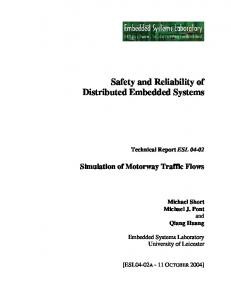
The simulations are carried out by resolving the whole boundary layer including the viscous sub-layer. The computational domain is of size 4 × 2 × 1 m3 in the streamwise (x), spanwise (y) and vertical (z) directions, respectively. In standard LES, without using any near-wall treatment, the required grid resolution is ∆x+ ' 100, ∆y + ' 30 and ∆z1+ ' 1 (wall-adjacent cell centers) (Davidson, 2009). However, LES of high Reynolds number flows using such fine grid-spacing is simply computationally too demanding even using modern supercomputing resources. Table 2.1 gives the information on the computational domain and grid system used in the LES of fully developed turbulent channel flows at smaller Reτ = 180 and Reτ = 395. It must be mentioned that the computational domain of channel flow studied here is different than, for example, it is used in the Direct Numerical Simulation (DNS) study of the turbulent channel flows by Moser et al. (1999). In this study, the domain consists only the lower-half part of the domain used in the DNS study. Therefore, only the lower-half part of the full-channel domain (Moser et al., 1999) is simulated here by imposing the slip boundary condition at top surface of the domain. In this situation, the computational domain-height d equals to one boundary-layer depth δ for the periodic channel flow. The flow studied here is also sometimes known as open channel flow and is an important model problem with relevance to many environmental and industrial applications (Taylor et al., 2005). In the LES calculations, flow is driven by a uniform pressure gradient aligned with the streamwise direction, and periodicity is applied in both horizontal directions while no-slip boundary condition is used at the bottom surface. Figures 2.1 and 2.2 compare the LESpredicted results with the DNS data (Moser et al., 1999) of the channel flows for Reτ = 180 and Reτ = 395, respectively. As seen from Figures 2.1(a) and 2.2(a), the LES prediction of the mean flow excellently reproduces the DNS data in both cases. The maximum difference (or relative error) between the LES and DNS solutions of the mean flow is 2.6%. The LES prediction of the Reynolds stress also agrees with the DNS data for most of the components. Only the prediction of the hu0 u0 i component overestimates the DNS data mostly away from the wall in both cases. The overestimation is stronger in the case of Reτ = 395, partially due to the coarser grid

2. LES methodology

26

Table 2.1: Information on the domain size and grid number used in LES of fully developed turbulent channel flows.

LES cases

Domain size in in x, y and z directions 4×2×1m

Reτ = 395

4 × 2 × 1 m3

1

LES:Reτ=180 U+=(1/κ)ln(z+)+5.45

0.8

U+=Z+ DNS

+



+



0.6

+



z/δ

U+

15

Non-dimensional grid spacing

∆x+ = 14.4 50 × 50 × 50 ∆y + = 7.2 + ∆z = 0.91 − 9.13 ∆x+ = 19.5 80 × 80 × 80 ∆y + = 9.87 + ∆z = 0.54 − 17.5

3

Reτ = 180

20

Number of grid cells

10

+

DNS

0.4

5

0 −1 10

0.2

0

10

1

10 z+

2

10

0 −1

3

10

0

(a) Mean velocity

1

2

3 4 /u2τ

5

6

7

8

(b) Reynolds stress

Figure 2.1: LES results compared with DNS data by Moser et al. (1999) for fully developed channel flow at Reτ = 180. The symbols represent the DNS data.

25 20

1

LES:Reτ=395 U+=(1/κ)ln(z+)+5.45

0.8

U+=Z+ DNS

+ 0.6

+

10

0.4

+ DNS

5

0.2

+

z/δ

U+

15

0 −1 10

0

10

1

10 z+

(a) Mean velocity

2

10

3

10

0 −1

0

1

2

3 4 /u2τ

5

6

(b) Reynolds stress

Figure 2.2: LES results compared with DNS data by Moser et al. (1999) for fully developed channel flow at Reτ = 395. The symbols represent the DNS data.

7

8

2.5 Wall-function model

27

spacing (∆z + ) used in the vertical direction near the top boundary compared to that of in the case of Reτ = 180. For both cases, the overestimation is strongly owing to the slip boundary condition applied at the top surface of the domain. The slip condition imposes the zero-gradient (Neumann type) boundary condition for a scalar quantity; but for a vector quantity, the normal component is zero, whereas the tangential components are zero-gradient. This means in the present channel-flow simulations the boundary condition for velocity leads to d˜ u/dz = d˜ v /dz = 0 and w˜ = 0. Thus, the slip-condition does not allow the fluid to flow normal to the top surface, which is not a case in the DNS calculations. Due to this, the flow behaves differently in LES than in DNS near the top boundary, and thus the comparison is meaningful only in the near-wall region.

2.5

Wall-function model

The boundary layer can generally be divided in two parts. The first part is the inner nearwall region, where the flow is viscous-dominated and thus Reynolds number dependent over aerodynamically smooth surfaces and controlled by the roughness over fully rough surfaces. The second part is an outer region away from the wall. In high Reynolds number flows such as the present atmospheric flows over complex terrain, resolving all the dynamically influential eddies in the inner-layer is simply impossible. On the other hand, the grid-resolution requirement of the outer region is relatively small and is essentially independent of the Reynolds number (Bechmann, 2006). Therefore, in order to perform LES at high Reynolds numbers, wall-function models have been introduced to supply boundary conditions to LES in an effort to eliminate the need of fully resolving the surface layer. Even more importantly, the wall surface in ABL flows is not smooth but consists of roughness elements. Different types of ground surfaces, such as soil, vegetation, sand and stones, sometimes even water surface, are impossible to be described and resolved directly even using fine computational mesh, then their effects to wind flow must be approximated using wall functions. Therefore, to make LES computationally affordable for simulating atmospheric flow over complex terrain a wall function approach is necessary, and has been adopted in the present work. 2.5.1 Smooth wall function Blocken et al. (2007) have addressed the applications and problems using a wall-function R approach in CFD simulation of ABL flows. For the LES modeling, however OpenFOAM offers only one wall-function model called nuSgsUSpaldingWallFunction which is based on the Spalding’s proposed formula (Eq. (2.23)) for the law of a smooth wall (Spalding, 1961; OpenCFD, 2013).   1 1 1 κU + + + 2 + 3 + + e − 1 − κU − (κU ) − (κU ) , (2.23) z =U + E 2 6 where κ = 0.41 is the von Kármán constant, E = 9.1 is a constant value, U is the mean velocity, z + is the non-dimensional vertical height. The Spalding’s formula fits to the laminar, buffer and logarithmic regions of an equilibrium boundary layer (De Villiers, 2006).

28

2. LES methodology

Ideally, any wall-function based on the logarithmic law of a smooth wall (Eq. (2.24)) should not be used in the simulations of flows over complex terrains, as the surface is highly rough due to roughness elements mentioned earlier. Instead of that, the logarithmic law of a rough wall (Eq. (2.25) or Eq. (2.31)) depending on the aerodynamic roughness-length z0 or the sand-grain roughness height ks should be used in such simulations. The mean logarithmic velocity profile over a smooth surface can be defined as z · u  uτ τ ln +C U= κ ν and over a rough surface as   uτ z U= ln κ z0

(2.24)

(2.25)

where uτ is the friction velocity, C = 5 − 5.5 is the constant for a smooth wall, and z0 is the ground roughness length. Under the fixed value of uτ , Eqs. (2.24) and (2.25) lead to different mean velocity profiles, although they have same slope. The difference in the mean velocity between the smooth and rough boundary-layer profiles is shown in Figure 2.4. In that context, although the wall function nuSgsUSpaldingWallFunction does not represent the reality for the rough boundary-layer flow typical in ABL, several test cases are made using the newly developed solver rk4ProjectionFoam in order to study and to validate the wall-function methodology with coarse grid resolutions for turbulent boundary-layer flows at different Reτ values. The test cases are carried out in a channel of size 4 × 2 × 1 m3 on a coarse Cartesian grid. In practice when using a wall-function approach in simulations, the center of the walladjacent cell with height zp is placed in the logarithmic layer, typically zp+ > 30. However, the requirement of zp+ certainly depends on the type of the wall function being used in the simulation. For the present cases, the information on the total number of computational grid cells together with non-dimensional grid spacing is given in Table 2.2. The nondimensional grid spacings (∆x+ , ∆y + and ∆z + ) chosen in the test cases are typical when using a wall-function approach and they are adopted from the literature (Cabot and Moin, 2000; Nikitin et al., 2000; Templeton, 2006; Piomelli and Balaras, 2002; Davidson, 2009, 2010). However, the aim of the test cases is to examine the LES solver using wall-function modeling by reproducing the mean flow solution under different Reynolds number (Reτ ) flows. In all test cases listed in Table 2.2, the flow is driven by a pressure gradient aligned with the streamwise direction and periodic boundary conditions are applied in both streamwise and spanwise directions. A slip boundary condition is imposed on the top boundary, whereas the smooth-wall function is used on the lower boundary of the domain. The LES predicted mean velocity profiles from the test cases are compared with the standard log-law of a smooth wall (Eq. (2.24)) in Figure 2.3. From Figure 2.3, it can be observed that the overall LES prediction follows the analytical solution, i.e. the log-law of a smooth wall (Eq. (2.24)), in all cases. The LES solution is correct at the first grid point, but after that however an artificial layer develops near the wall only over the next few grid points after the first one, where a matching with the log-law is

2.5 Wall-function model

29

Table 2.2: Information on the domain size and grid used in the test cases of nuSgsUSpaldingWallFunction for the smooth boundary-layer flows in channel.

LES cases

Domain size in in x, y and z directions 3

Reτ = 10000

4×2×1m

Reτ = 21000

4 × 2 × 1 m3

Reτ = 60000

4 × 2 × 1 m3

Number of grid cells

Non-dimensional grid spacing

∆x+ = 500 80 × 60 × 60 ∆y + = 333.3 ∆z + = 83.3 − 300 ∆x+ = 840 100 × 100 × 100 ∆y + = 420 ∆z + = 210 ∆x+ = 937.50 256 × 256 × 128 ∆y + = 468.75 ∆z + = 468.75

not perfect as LES under-predicts the mean velocity. After the so-called artificial viscouslike layer, again the LES profile agrees with the log-law. This deficiency of the prediction in near-wall region does not seem to improve by using fine grid spacings. Also, it seems to be independent of the Reynolds number as it appears in all the solutions shown in Figure 2.3. This is indeed a typical problem in LES using a wall-function approach. Not all but several previous LES studies have discussed the same issue (Templeton, 2006; Nicoud et al., 2001; Piomelli and Balaras, 2002; Temmerman et al., 2003; Piomelli, 2008; Davidson, 2010) and it is still on-going research topic for the LES community. For example, Davidson (2010) proposed a wall-function model coupled with backscatter (forcing) from a scale-similarity model. He showed improvement in the case of channel flow but no additional improvement was observed in a 3D hill case with a flow separation. 2.5.2 Implementation and validation of new wall-function for a rough surface condition As mentioned previously, in cases of real complex topographies, the surface is not smooth but highly rough with a combination of different roughness elements. It is impossible to use such a fine computational mesh that resolves all the individual local roughness elements located on the terrain surface. One way is to model their effect on the flow by describing their aerodynamic roughness length z0 or sand-grain roughness height ks using a wall function. In the present work, in order to perform LES over complex terrain, a new wall-function boundary condition, called here ABLRoughWallFunction, based R on the Eq. (2.25) is implemented into OpenFOAM and has been employed here together with solver rk4ProjectionFoam. For the implementation of the new wall-boundary condition, we follow the same approach as used for another existing wall function in R OpenFOAM . Using ABLRoughWallFunction, the instantaneous wall shear stress τw is implemented by prescribing the kinematic SGS viscosity νsgs at the wall boundary by using the logarith-

2. LES methodology

30

35

35 LES:Reτ=10000

30

LES:Reτ=21000

30

U+=(1/κ)ln(z+)+5.45 U+

25

U+

25

U+=(1/κ)ln(z+)+5.45

20

20

15

15

10 1 10

2

10

3

4

10 z+

10 1 10

5

10

10

(a) Mean velocity for Reτ = 10000

2

3

10

10 z+

4

10

(b) Mean velocity for Reτ = 21000

35 LES:Reτ=60000

30

U+=(1/κ)ln(z+)+5.45

U+

25 20 15 10 1 10

2

10

3

10 z+

4

10

5

10

(c) Mean velocity for Reτ = 60000 Figure 2.3: LES predicted mean velocity profiles obtained using the smooth wallfunction model for the channel flows at different Reτ values.

5

10

2.5 Wall-function model

31

mic law of a rough wall (Eq. (2.25)) but in a strictly instantaneous sense, that is   z uτ ln u˜ = κ z0

(2.26)

where u˜ is the instantaneous LES resolved velocity. The wall shear stress can be defined using an effective viscosity µef f = (µ + µsgs ) such that τw = (µ + µsgs )

u˜p d˜ u ≈ (µ + µsgs ) dz zp

(2.27)

where µ is the fluid viscosity, µsgs is SGS viscosity and subscript p indicates the values at thep first interior nodes from the wall. Using the definitions of the frictional velocity uτ = τw /ρ and the kinematic viscosity ν = (µ/ρ) into the Eq. (2.27), we get u2τ = (ν + νsgs )

u˜p . zp

(2.28)

Consequently, the kinematic SGS viscosity νsgs at the wall can be calculated as νsgs =

u2τ −ν (˜ up /zp )

(2.29)

in which uτ follows from the the Eq. (2.26), as shown below uτ =

u˜p κ . ln (zp /z0 )

(2.30)

Table 2.3: Information on the domain size and grid spacing used in the validation cases of ABLRoughWallFunction for the rough boundary-layer channel flows. LES cases Domain size Number of Non-dimensional Roughness length grid cells grid spacing z0 (m) Reτ = 7500

4×2×1

m3

50 × 50 × 25

Reτ = 10000

4 × 2 × 1 m3

66 × 66 × 33

∆x+ = 600 ∆y + = 300 ∆z + = 300 ∆x+ = 606 ∆y + = 303 ∆z + = 303

0.000444

0.000444

R The wall function ABLRoughWallFunction implemented into OpenFOAM is validated together with rk4ProjectionFoam by simulating the fully developed rough boundary-layer flows at two different Reτ = 7500 and Reτ = 10000 values. Table 2.3 gives the information on domain, grid and roughness length used in the validation cases. Figures 2.4(a) and 2.4(b) compare the simulated mean streamwise velocity profile with the logarithmic laws of the smooth and rough walls given in Eq. (2.24) and Eq. (2.25), respectively. The mean velocity profile over fully rough surface can also be defined as (Blocken et al., 2007)  +   U 1 1 z z = ln + 8.5 ⇒ ln + 8.5 (2.31) + uτ κ ks κ ks

2. LES methodology

32

where ks is the sand-grain roughness height. It is pointed out that Eq. (2.31) is another form of the logarithmic law of fully rough surfaces which does not depend on aerodynamic roughness length (z0 ) but sand-grain roughness height (ks ). However, both logarithmic laws, Eq. (2.25) and Eq. (2.31) are equal using the relation ks = e8.5κ z0 .

(2.32)

Then, using κ = 0.41 in above equation, one would find ks = 32.62z0 . Based on the non-dimensional roughness height ks+ (= ks · uτ /ν) value, three regimes of the flow are distinguished: aerodynamically smooth (ks+ ≤ 2.25), transitional (2.25 ≤ ks+ < 90) and fully rough (ks+ ≥ 90) (Blocken et al., 2007). In the present validation cases, the non-dimensional roughness height (ks+ ) equals to 108.62 and 144.83 in the case of Reτ = 7500 and Reτ = 10000, respectively. This means the flow simulated here is fully rough in both cases. According to Figure 2.4, LES using the newly implemented wall-function boundary condition reproduces the logarithmic velocity profile (Eq. (2.25)) of a rough surface for both Reynolds numbers. Note that the problem of the artificial viscous-like layer, as seen previously in Figure 2.3, still exists using the roughwall function. Moreover, a clear difference between the smooth and rough boundary-layer profiles can be seen in the figures. Further, the difference would likely to be much higher in the simulations at real scale depending on the roughness parameter and thus it is very important to use a rough-wall boundary condition. 30

30

LES: Reτ=7500

LES: Reτ=10000

+

U =(1/κ)ln(z/z0)

25

U+=(1/κ)ln(z/z0)

25

U+=(1/κ)ln(z+)+5.45

U+

20

U+

20

U+=(1/κ)ln(z+)+5.45

15

15

10

10

5 2 10

3

10 z+

(a) Mean velocity for Reτ = 7500

4

10

5 2 10

3

10 z+

(b) Mean velocity for Reτ = 10000

Figure 2.4: LES predicted mean velocity profiles obtained using the rough wallfunction for the channel flows at two Reτ values.

2.6

Inflow boundary condition

Apart from the wall boundary condition, the realistic inflow (upstream) boundary condition is also one of the major difficulties in LES. The upstream velocity boundary condition must contain turbulent fluctuations as a function of space and time with a realistic energy distribution over the spatial directions and the simulated wave-number range. The turbulence structure in the upstream boundary condition plays an important role in predicting

4

10

2.6 Inflow boundary condition

33

local flow details accurately around a complex topography. It is therefore necessary to find upstream boundary conditions more appropriate and realistic than those utilized in the previous studies. There are a number of methods to generate the inflow turbulence such as a synthetic turbulence or the use of a periodic boundary condition in the streamwise direction. LES for atmospheric flows over flat terrains with homogeneous roughness are often performed by using a periodic boundary condition in the streamwise direction. However, periodic boundary conditions can not be used in the simulations of flow over terrains with inhomogeneous surface conditions, which is always the case in a complex topography. The most accurate way of generating the genuine inflow turbulence is to run a so-called precursor simulation, either before the main simulation or simultaneously with it. In the former case, a separate precursor LES with periodic boundary conditions in streamwise direction is carried out over the flat terrain and the instantaneous field data is stored separately on the hard disk at each time step to create a library of turbulence or inflow velocity data. The stored data is then used as the fully developed upstream boundary condition for the terrain simulation (successor). This method is previously used in several LES studies (Bechmann, 2006; Bechmann et al., 2007; Silva Lopes et al., 2007; Krajnovi´c, 2008; Chow and Street, 2009; Bechmann and Sørensen, 2010; Diebold et al., 2013). In the present study, a variant of the latter method, which is so-called recycling (or mapping) method, is employed for simulating ABL flows over complex terrains. In this method, the precursor simulation is combined with the main (terrain) simulation as shown in Figure 2.5. During the simulation, the flow variables are sampled on a cross-stream plane (Recycling plane in Figure 2.5), which is sufficiently far downstream from the inflow plane, and the sampled data are then recycled back to the inflow plane at each time step. The recycling technique develops the upstream boundary-layer flow together with the inflow turbulence simultaneously with the main simulation and within a single computational domain. In addition to recycling, the volume flux is fixed on the inflow boundary so that it will maintain the same amount of a volumetric flow throughout the simulation. By recycling the flow data from further downstream a recycling section is created in which the flow becomes fully developed and at the same time the flow within this section is automatically fed into the main domain. The method is simple to implement into LES code and easier to manipulate for each different inflow boundary-condition requirements. The method is explained in detail by Baba-Ahmadi and Tabor (2009), and they also presented validation of the method for turbulent channel and pipe flow simulations. Note that in the literature, a number of different variants of the recycling method have been reported previously. For example, Lund et al. (1998) and later Nozawa and Tamura (2002) have proposed similar methods for generating the inflow turbulence. Tamura et al. (2007) and Cao et al. (2012) have used this method to generate upstream boundary conditions for their two-dimensional hill flow simulations, which is somewhat different from the present recycling method. Their method rescales the velocity field at a downstream station and reintroduces it as a boundary condition at the inflow plane. Also, their method uses two separate computational domains, one for generating the upstream boundary condition and the other for the hill flow simulation. However, there is no reason why the recycling has to be done on two separate flows (or domains) rather than on the main domain itself, which will reduce the cost of calculation both in terms of computational time and storage require-

34

2. LES methodology

ment (Baba-Ahmadi and Tabor, 2009). Mayor et al. (2002) proposed "perturbation recycling method" which is also slightly different than the one used here. In that method, the mean flow conditions are imposed at the inflow plane and only the turbulent perturbations are sampled from the downstream plane and are recycled at the inflow plane. Golaz et al. (2009) used another alternative that employs total of two grids, a parent grid and a one-way nested grid. They utilized this approach to simulate wind flow over the Askervein hill. The parent grid has a flat terrain and uses periodic boundary condition in the streamwise direction. The nested grid contains the terrain to be simulated and is forced at its boundaries by the parent grid. The parent grid then continuously provides a turbulent inflow to the nested grid. It is worth to remind that a number of different variants of the recycling method exist, such as those described by Lund et al. (1998), Nozawa and Tamura (2002), Mayor et al. (2002) and Golaz et al. (2009), but the technique discussed here is somewhat different than the other previously reported variants. The main advantage of the present technique is that precursor simulations on separate meshes can be avoided, and thus simulations can be carried out on a single computational domain or grid without any modification to the recycled R flow. The method is already implemented into the standard release of OpenFOAM with a term called mapped (OpenCFD, 2013).

Figure 2.5: Schematic picture of computational model showing the generation of upstream boundary condition.

Using the proposed recycling method, some tests were performed for simple flows to estimate the minimum acceptable recycling length or distance Lrcy between the inflow plane and the recycling plane. This was important in order to avoid unnecessary recycling length, which will help to reduce the total length of the computational domain. It should be mentioned that none of the previous studies have provided this kind of estimation of the minimum acceptable length required for recycling method. The test cases were carried out by simulating the channel flows with varying recycling lengths. During all the test cases, the computational domain-height Lz was fixed to some value d and the domain-width Ly to 2d, but the domain-length Lx was varying according to the recycling-lengths. Here, d being the vertical height of the domain. Moreover, the depth of the boundary-layer δ was

2.6 Inflow boundary condition

35

assumed to be the domain-height, i.e. δ = d, in all the test cases. For example, Figure 2.5 illustrates the computational domain of the test case carried out with Lrcy = 3δ = 3d. This test was carried out in a domain of size 5d × 2d × d using a grid 120 × 48 × 32 in x, y and z directions, respectively. Moreover, the static pressure was fixed to a constant value on the outlet plane, while the Neumann boundary condition was used for the rest of the flow variables. The slip boundary condition was used for all the flow variables at the top boundary, whereas periodic boundary conditions were employed in the spanwise (y) direction. The smooth-wall function boundary condition was used at the lower surface. From a number of test cases performed by varying the recycling-lengths, it was found that Lrcy should be at least 3δ, to ensure that this distance is larger than the streamwise length of the largest turbulent structures. Figure 2.6 shows the instantaneous flow structures at wall-parallel planes with three recycling lengths: 4δ, 3δ and 1δ. As seen in Figure 2.6(c), the flow contains some kind of artificial structures such as periodicity, because of the short recycling-length (Lrcy = 1δ). The insufficient or short recycling-length does not allow the flow structures to be changed significantly within a distance from inflow plane to recycling plane. In the cases with Lrcy = 3δ (Figure 2.6(b)) and Lrcy = 4δ (Figure 2.6(a)), the turbulence structures are more developed and look realistic compared to the shortest recyclinglength (Lrcy = 1δ). Especially using the longest recycling-length (Lrcy = 4δ), the flow structure is expected to be the best among all the recycling-lengths. Thus, according to Figure 2.6, recycling length of 1δ seems to be insufficient but a recycling-length Lrcy ≥ 3δ would be expected to be sufficient when using the recycling technique for developing the upstream boundary-layer flow with inflow turbulence. The results from a test case carried out with Lrcy = 3δ were further post-processed and are reported here as a validation of the upstream boundary-condition method. Figures 2.7 and 2.8 show the vertical profiles of the mean velocity U and the resolved Reynolds shear stress −hu0 w0 i at different locations in the streamwise (x) direction. Here, all the results are space averaged along the spanwise direction and are normalized using the frictional velocity. As seen in the figures, the mean flow is fully developed and the LES profiles agree well with the logarithmic law of the wall at all the locations, before and after the recycling plane. Moreover, the shear stress profile also remains steady throughout the whole domain. Thus, within a short distance an equilibrium boundary-layer flow is obtained. This obviously is a direct consequence of using the recycling method. Hence, this method is employed in all the LES calculations reported in this study.

36

2. LES methodology

Figure 2.6: Instantaneous streamwise velocity contours showing the turbulence structures at wall-parallel (x − y) planes with different recycling lengths: (a) Lrcy = 4δ, (b) Lrcy = 3δ and (c) Lrcy = 1δ. The planes are taken at the height z/δ = 0.5.

2.6 Inflow boundary condition

0

x/δ=0.5

37

x/δ=2.5

x/δ=1.5

x/δ=3.5

x/δ=4.5

z/δ

10

−1

10

U=(uτ/κ) ln(z+)+5.45 LES

−2

10

16

20

24

28

U/uτ

Figure 2.7: Vertical profiles of the non-dimensional mean velocity U/uτ compared with the logarithmic law (Eq. (2.24)) at different locations in the streamwise direction.

x/δ=0.5

x/δ=1.5

x/δ=2.5

x/δ=3.5

x/δ=4.5

1 0.8

z/δ

0.6 +

0.4 0.2 0 −1

2 0 /uτ

Figure 2.8: Vertical profiles of the resolved Reynolds shear stress −hu0 w0 i at different locations in the streamwise direction.

38

2. LES methodology

C HAPTER III

Flow over two-dimensional wind-tunnel hills

3.1

Background

This thesis is oriented towards LES for ABL flows over complex terrains. However, a systematic study of the boundary-layer flow over idealized hilly terrains by means of LES is a necessary step towards better understanding the flow and how to simulate it over realistic complex terrains. It is therefore desirable to first validate LES results against the wind-tunnel measurements to get confidence in our LES model and that is the objective of this chapter. Here, LES are carried out for the turbulent neutral ABL flow over the twodimensional wind-tunnel hill profiles or ridges with two different slopes. Indeed, there are many situations in nature such as a hill, a ridge or a group of hills with a practically constant cross section and a straight crest line, with wind flowing perpendicularly to this line, where a two-dimensional approach can be accepted with a reasonable degree of accuracy (Ferreira et al., 1995). A turbulent flow over a steep hill contains moderately complex mean-flow characteristics such as separation and reattachment. As the flow passes over the hill, a recirculation region can be formed behind the hill and turbulence is enhanced in the wake region. Thus, it is important to detect the influence of the different hill shapes on overall flow behavior over hilly terrains. Furthermore, the condition of the hill surface, smooth or rough is an important factor while studying the effects of topography. After reviewing many field observations and wind-tunnel experiments, Finnigan (1988) pointed out that the occurrence of a flow separation in the wake region depends on the hill shape (2D or 3D), steepness and roughness conditions. For simulating flow over the hills, correct predictions of the flow separation point, the length of the recirculation region and the turbulence production are the typical difficulties involved with the numerical simulations. Thus, the experimental validation of numerical predictions of wind flow over a steep hill is of utmost importance. Many researchers have performed wind-tunnel experiments to investigate the wind flow structures over twodimensional hills or ridges using various techniques (Britter et al., 1981; Khurshudyan et al., 1981; Ferreira et al., 1995; Kim et al., 1997; Ross et al., 2004; Cao and Tamura, 2006; Loureiro et al., 2007; Houra and Nagano, 2009; Conan, 2012). For example, Khurshudyan et al. (1981) carried out the wind-tunnel experiment (the RUSHIL experiment) by 39

40

3. Flow over two-dimensional wind-tunnel hills

employing the hot-wire anemometry and studied the ABL flows over three different isolated two-dimensional hills under the neutral atmospheric condition. The experimental data can be found in ERCOFTAC data base (Ercoftac, 2013). After the RUSHIL experiment, there have been several attempts to simulate this particular wind-tunnel experiment by using RANS (Castro and Apsley, 1997; El Kasmi and Masson, 2010; Finardi et al., 1993; Ying and Canuto, 1997; Agafonova et al., 2014) and LES (Allen and Brown, 2002; Chaudhari et al., 2014b,c) approaches. The numerical results from all these studies are compared with the RUSHIL wind-tunnel measurements (Khurshudyan et al., 1981). Because several comparisons already exist in the literature, the same wind-tunnel measurements are used here to compare the LES results regardless of the age of the wind-tunnel experiment. This will give us the opportunity to compare the LES results with the other numerical results performed in the past for the same hills in addition to the RUSHIL measurements. In addition, there are several other RANS studies dealing with numerical simulations of flows over isolated two-dimensional hills with varying slopes, and combinations of a hill and a building (Apsley and Castro, 1997; Griffiths and Middleton, 2010; Kim et al., 1997, 2001; Loureiro et al., 2008). Numerical simulations using RANS-based models have been the traditional technique for mean flow prediction in the most of engineering applications. The RANS-based numerical studies have been reported to predict the mean flow reasonably well, but most of the studies report a poor prediction of turbulence quantities, and they also underestimate the flow separation on the lee side of the hill. An alternative way to capture turbulence in the separation region is to use LES as it resolves the most important turbulent eddies and models only the small scale motions which are more universal. Thus, the use of LES to simulate complex flow configurations is becoming increasingly common nowadays. Gong et al. (1996) were the first to attempt LES of a neutral flow over aerodynamically fully rough hills, and showed that LES results agreed with the wind-tunnel measurements. Subsequently, Henn and Sykes (1999) did a similar study but for a smooth surface condition. Brown et al. (2001) performed LES for a turbulent flow over a rough sinusoidal ridge, but their work was limited to ridges not steep enough to cause flow separation. Allen and Brown (2002) simulated the turbulent flow over two-dimensional isolated and periodic hills. For the isolated two-dimensional hill, they compared LES results with the RUSHIL measurements (Khurshudyan et al., 1981), and reported that their LES model did not perform well on the lee side. Wan et al. (2007) studied the performance of SGS models for a neutral turbulent flow over a two-dimensional hill. Furthermore, Tamura et al. (2007) and Cao et al. (2012) carried out LES studies on the turbulent boundary layer flow over two-dimensional sinusoidal hills of different sizes for smooth and rough surfaces. Although both these studies are close to each other, there are a few noticeable differences between them, e.g., the use of different grids and different Reynolds numbers. Both LES studies show a fair agreement with the experimental results of Cao and Tamura (2006). For flow over the two-dimensional hill, the roughness factor is carefully studied by Tamura et al. (2007) and Cao et al. (2012), and they reported that the separation region formed in the wake of the rough hill is larger than that formed in the wake of the smooth hill. In both studies, the roughness effect was studied by explicitly simulating small roughness blocks with their geometrical shapes. The roughness blocks were placed on the surface throughout the entire computational domain. This technique is perhaps most suitable for developing the fully rough boundary-layer flows with the roughness-block enhanced turbulence in

3.1 Background

41

LES. However, explicit modeling of the roughness blocks is restricted to smaller Reynolds number flows where the viscous sub layer can be resolved, and this could possibly lead to Reynolds number dependent results. Thus, it may not be representative of the real wind flow over real hill. In the present study, roughness elements are modeled implicitly, that is, the actual elements are not included in the domain, but the corresponding value of roughness length z0 is implemented using a wall function. In this way, the roughness effect is modeled in the flow and at the same time the flow with higher Reynolds number (or independent of Reynolds number) is also possible to simulate. Concerning the upstream boundary condition, Tamura et al. (2007) demonstrated that the behavior of the separated shear layer and the vortex motions are affected by the oncoming turbulence, such that the shear layer comes close to the ground surface, or the size of a separation region becomes small because of the earlier instability of the separated shear layer (Tamura et al., 2007). Also, Krajnovi´c (2008) suggested that the flow around the curved shaped obstacles such as a hill is very sensitive to the upstream boundary-layer development. This implies that the inflow turbulence plays an important role in order to accurately predict the flow separation and turbulence properties behind the hill. Because of the difficulty of imposing realistic upstream boundary condition in LES, a periodic boundary condition in the streamwise direction is often used (Allen and Brown, 2002; Wan et al., 2007). In the case of the isolated hill, however a periodic boundary condition is not suitable as the flow involves large separation, unless a long computational domain is used to remove the wake structures generated by the hill, as pointed out by Tamura et al. (2007). However, Allen and Brown (2002) used periodic boundary condition for simulating a flow over the isolated hill of the RUSHIL experiment. Their LES results underestimate the size of the recirculation region compared to the measurements. In our opinion, use of a periodic boundary condition would not be realistic since the wake of a hill certainly extends much further downstream which will influence the inlet condition when using a periodic boundary condition. Recently, Chaudhari et al. (2014b) carried out LES for turbulent boundary-layer flows over the same RUSHIL experimental hills but for smooth surface conditions. The study was performed for a low Reynolds number flow by resolving the viscous sub-layer. The inflow boundary condition was developed by imposing the fully developed mean velocity profile with artificially generated perturbations because the recycling technique was not available in the commercial software ANSYS Fluent (Ansys, 2010). The artificial perturbations were generated using the so-called random 2D vortex method (Ansys, 2010) leading to constant turbulence intensity of 12%. However, this type of inflow boundary condition does not represent the reality and thus it is also not convincing to be used especially for the flow over a real terrain. To overcome this issue here, the flow recycling technique, described in the previous chapter, is employed to develop the upstream boundary layer for the same hill geometries, i.e. the RUSHIL wind-tunnel hills. By this way, one can also see the influences of the two inflow boundary conditions in the same flow problem. In this chapter, LES are performed to investigate the turbulent boundary-layer flows over mainly aerodynamically rough two-dimensional hill profiles or ridges of two different slopes. The hill shapes used here are the same as those used in the RUSHIL experiment (Khurshudyan et al., 1981) and the LES results are compared with their measurements. The upstream boundary condition used in this study is different and more realistic than the one used in the previous LES studies of these types of hill flows. Moreover, the Reynolds

3. Flow over two-dimensional wind-tunnel hills

42

number ReH based on the hill height and the free stream velocity is 31200 which equals to the wind-tunnel Reynolds number and is higher than in some previous LES calculations (Henn and Sykes, 1999; Tamura et al., 2007; Cao et al., 2012; Hattori et al., 2013; Chaudhari et al., 2014b). Although the focus of work is the wind flow over aerodynamically rough hills, a number of other LES calculations for the flow over smooth hills are also carried out in order to elaborate the sensitivity of the flow with wall-function model.

3.2

Computational set-up

3.2.1 Computational domain and grid Khurshudyan et al. (1981) carried out the RUSHIL experiment that simulates the neutral atmospheric boundary layer flows over the three different isolated two-dimensional hills of varying slopes. During the laboratory experiment, the inflow profile was characterized by the well-known logarithmic velocity profile (also Eq. (2.25))   z u∗ ln (3.1) u= κ z0 where u∗ = 0.178 m/s is the friction velocity, and z0 = 0.000157 m is the roughness length. From here on, the friction velocity is referred as u∗ instead of uτ . At the windtunnel scaling ratio 1/500, the roughness length equals to 0.0785 m which corresponds to tall grassland or crops in full scale. This means the roughness is sufficient to maintain the fully rough turbulent boundary layer. The data from the RUSHIL experiment is available for the three different hills of varying slopes. Among the three hill slopes of the RUSHIL experiment, the shallowest hill is not studied here as it is not expected to cause any flow separation, according to Khurshudyan et al. (1981). Hence in this thesis, the first two steepest hills are studied. The hill height H is fixed to 0.117 m in both cases but the hill half-length a varies from 3H to 5H, as shown in Figure 3.1. The shapes of the hills can be reproduced by the parametric formulae given in Eqs. (3.2), (3.3) and (3.4).

x=

  a2 1 ξ 1+ 2 , 2 ξ + m2 (a2 − ξ 2 )

z=

  1 p 2 a2 m a − ξ2 1 − 2 , 2 ξ + m2 (a2 − ξ 2 )

(3.2)

for |ξ| < a

(3.3)

and z = 0, for |ξ| ≥ a, (3.4) √ where m = n + n2 + 1, and n = H/a is the average slope. Khurshudyan et al. (1981) is referred for the further details on the experiment. The two hill shapes used here are named as Hill3 and Hill5 according to the ratios a/H, and the corresponding maximum hill slopes are 26◦ and 16◦ , respectively. Hill3 is the steepest one, the flow over it is characterized by x = ξ,

3.2 Computational set-up

43

a massive flow separation on the lee side. According to Tamura et al. (2007), the critical slope for the existence of a flow separation is reported to be 16◦ which is the maximum slope of Hill5. For this reason in Hill5, the flow is just on the verge of a separation. This means that the flow separation is likely to be very sensitive to small inaccuracies, such as the upstream boundary conditions, roughness, the Reynolds number and other numerical details. Therefore, it is probably very challenging for a numerical simulation to predict the flow accurately especially on the lee side.

z/H

2 Hill3 Hill5

1 H

0 −5

−4

−3

−2

−1

0

1

2

3

4

5

x/H

Figure 3.1: Shapes of the hill models (Hill3 and Hill5).

In the wind-tunnel experiment, the hill models were covered with river-washed gravel to match the roughness. Therefore, the interest here is to simulate the boundary-layer flows over the rough hills with the roughness length given in Eq. (3.1). But, both hill-shapes are also studied here with the smooth surface conditions in addition to the rough surface conditions. The height Lz of the computational domain is set to 1 m and the depth of the boundary layer δ is also 1 m (i.e. Lz = δ = 8.547H). In the spanwise (y) direction, the computational domain is spanned twice the boundary-layer depth, i.e. Ly = 2δ = 17.09H in order to perform fully three-dimensional (3D) LES. Figure 3.2 shows the full 3D computational domain used in the simulation of flow over Hill3. Note that Lx , Ly and Lz are the lengths of the computational domain in the streamwise, spanwise and vertical directions, respectively. In all the LES calculations reported in this chapter, the computational domain is discretized using a block-structured hexahedron mesh with finer grid resolution on the hill. The grid resolution is selected so that the center of the wall-adjacent cell zp is located in the logarithmic region, i.e. zp+ > 30. This implies that the first mesh-node z1+ from the surface should be larger than 60, i.e. z1+ & 60 as z1 = 2zp . This grid resolution requirement is recommended to use when employing a wall-function approach especially based on the logarithmic laws (i.e. on Eqs. (2.24), (2.26) and (2.31)). Another grid requirement for a rough wall function (Eq. (2.31)), which is based on the roughness height ks , is that a distance zp should be larger than the physical roughness height of terrain, i.e. zp > ks (Blocken et al., 2007). Thus, in line with a wall-function modeling in the present case, the number of cells in the vertical direction is chosen to 70 and they are stretched such that the height of the + smallest (also the wall-adjacent) grid cell is 0.008 m (i.e. ∆zmin = ∆z1+ ≈ 95 and + ∆zmin = 0.0684H) and the largest cell height is 0.0296 m (∆zmax ≈ 351 and ∆zmax = 0.253H). The streamwise grid spacing ∆x is non-uniform with the minimum grid spacing + of ∆x+ min ≈ 173 on the hill surface and the maximum grid spacing of ∆xmax ≈ 276 near the inlet and outlet boundaries. The spanwise grid spacing is fixed to that of the minimum

3. Flow over two-dimensional wind-tunnel hills

44

Figure 3.2: Picture of the computational domain used in LES of flow over wind-tunnel hill (Hill3).

streamwise grid-spacing, i.e. ∆y + = ∆x+ min ≈ 173. More information on the computational domain and grid system with grid spacing in each direction is given in Table 3.1. Table 3.1: Information on the numerical domains and grid resolutions used in LES of flow over the two-dimensional hills. LES Domain Grid spacing and ReH Roughness Lx Ly Lz number of cells length (m) Case-A Rough

Case-B Smooth

Case-C Rough

8.34 (m) 71.28H

2 (m) 17.09H

1 (m) 8.547H

8.34 (m) 71.28H

2 (m) 17.09H

1 (m) 8.547H

8.34 (m) 71.28H

2 (m) 17.09H

1 (m) 8.547H

∆x = 0.125H − 0.199H ∆y = 0.125H ∆z = 0.0684H − 0.253H 495 × 136 × 70 ∆x = 0.125H − 0.199H ∆y = 0.125H ∆z = 0.0684H − 0.253H 495 × 136 × 70 ∆x = 0.0096H − 0.187H ∆y = 0.107H ∆z = 0.0684H − 0.17H 608 × 160 × 90

Roughness height ks+

31200

0.000157

60.77

31200

Smooth

Smooth

31200

0.000157

60.77

For both hill-shapes (Hill3 and Hill5), the simulations carried out over the rough hills are referred as Case-A and over the smooth hills as Case-B. As seen in Table 3.1, both cases (Case-A and Case-B) use the same size of computational domain and grid, hence the only difference between the two cases is the surface roughness. In addition to above, grid independent study was performed for the steeper hill case (Hill3) using a slightly finer grid consisting of 608 × 160 × 90 (≈ 8.75 × 106 ) cells, which is higher than the basic grid

3.3 Results and discussion

45

resolution 495 × 136 × 70 (≈ 4.71 × 106 ) used in Case-A or Case-B. The LES calculation performed using the finer grid is listed in Table 3.1 as Case-C, which is the same as CaseA (i.e. with rough surface) but uses a finer grid system compared to Case-A. However, Case-C was not performed for Hill5. 3.2.2 Boundary conditions For all the simulations, a fully developed upstream (inflow) boundary condition with realistic turbulence is generated using the recycling method. The static pressure is fixed to a constant value on the outflow plane, while the Neumann boundary condition is used for the rest of the flow variables. The slip boundary condition is used for all the flow variables at the top boundary. Moreover all the simulations use periodic boundary conditions in the spanwise direction. Only the wall boundary condition is different between the two cases: CaseA and Case-B. In Case-A, the logarithmic wall function ABLRoughWallFunction (Section 2.5.2) with the roughness length z0 = 0.000157 m, is utilized to determine the ground-surface fluxes on the ground-surface boundary. While, the smooth-wall function R nuSgsUSpaldingWallFunction, already existing in OpenFOAM , is utilized at the ground-surface boundary in Case-B. Case-C uses the same boundary conditions as those used in Case-A. For all the cases, the Reynolds number ReH based on H and U∞ is about 31200, where the value of U∞ is 4 m/s. The Reynolds number is the same as that in the RUSHIL experiment (Khurshudyan et al., 1981). All the simulations were run until the physical time of t = 100 s and all the quantities were time averaged over the last 50 s, which is approximately 20 advection times along the entire domain. It was checked in the Hill3 case that the flow statistics were converged after 50 s of time averaging. In addition to the time averaging, the results are space averaged over the spanwise direction.

3.3

Results and discussion

3.3.1 Upstream boundary-layer flow The recycling method allows to create a fully developed upstream flow without a precursor domain. However, it is necessary to ensure that the boundary layer flow on the upstream side of the hill is in reasonable agreement with the measurement data. Figure 3.3 shows the 2 simulated profiles of the mean velocity U/U∞ and the Reynolds shear stress −hu0 w0 i/U∞ at some longitudinal locations on the upstream side of Hill3. Here, the LES results of Hill3 from Case-A are normalized by U∞ and are compared with the RUSHIL flat terrain measurements (Khurshudyan et al., 1981). From Figure 3.3(a), it can be seen that the mean velocity is well reproduced by the recycling method in the simulation. The difference between the prediction and the measured data is rather small, less than 4%. According to Figure 3.3(b), the peaks of the resolved Reynolds stress profiles underestimate the measured peak by approximately 20%, but when accounting the modeled (sub-grid) part with the resolved one, the total (i.e. the resolved plus the modeled) Reynolds stress profiles reproduce the correct peak of the measured profile at z/H ≈ 0.3. Apart from the peak location, the total Reynolds stress profiles have

3. Flow over two-dimensional wind-tunnel hills

46

in general similar shapes to the measured profile, but underestimate the magnitude of the measured profile for 0.3 < z/H < 5. Despite of this underestimation, the upstream flow in the simulation is indeed fully developed as the profiles in different locations collapse on single curves. This obviously is a direct consequence of using the recycling method. Concerning the discrepancies, it is worth to report that the measured data used in Figure 3.3 are taken from the flat terrain measurements and thus they correspond to another experimental set-up, while in this study, a separate LES was not performed for the flat-terrain simulation but the numerical results from the existing hill-flow simulation (Hill3) are utilized to compare with flat-terrain measurements. 10

z/H

6

8 6 z/H

8

10

Measurement x/δ=−5 x/δ=−4 x/δ=−3 x/δ=−2

4

4

2

2

0 0

0.2

0.4

0.6 U/U∞

0.8

(a) Mean velocity U/U∞

1

1.2

0 0

0.0005

0.001 0.0015 −/U 2∞

0.002

0.0025

2 (b) Reynolds shear stress −hu0 w0 i/U∞

Figure 3.3: LES predicted profiles compared with measurements at some longitudinal locations upstream from Hill3 for Case-A. In the frame (b), the dashed lines represent the resolved part and the solid lines show the total (i.e. the resolved plus the modeled) Reynolds shear stress profiles.

3.3.2 Flow over the hills We start this section by visualizing the flow fields over the hills. Among the three cases: Case-A, Case-B and Case-C reported in this chapter, Case-A is meant to reproduce the wind-tunnel flows by LES and thus it is closer to the reality than Case-B which does not use any aerodynamic roughness at all. Note that Case-C also represents the wind-tunnel flows but it is aimed to check the sensitivity of the LES results to grid resolution. We therefore visualize the flow fields only for the rough hills (Case-A). Later in this section, the results from all cases are compared with the measurements. Figures 3.4 and 3.5 show the instantaneous and mean streamwise velocity distributions on longitudinal (x − z) planes of the rough hills (Case-A), respectively. The streamlines in Figure 3.5 show the major recirculation, and the mean flow separation and the reattachment locations. As seen from the mean flow distributions (Figure 3.5), when the flow reaches the hill summit it accelerates and continues downstream with the flow separation on the lee side of the hill. Because the shape of Hill3 is much steeper than that of Hill5, a relatively large region of a separated flow begins from x = 1.04H. Whereas in Hill5, comparatively

3.3 Results and discussion

47

small region starting from x = 2.40H occurs close to the surface. In the wind tunnel measurements, the separation point for Hill3 is slightly downstream to x = 0.75H which is slightly upstream from the predicted value.

u (instantaneous) -1 0 1 2 3 4 -1.9

4.9

(a) Hill3 u (instantaneous) -1 0 1 2 3 4 -1.9

4.9

(b) Hill5 Figure 3.4: Instantaneous streamwise velocity contours. Results are from Case-A.

Tamura et al. (2007) reported the flow separation point at x = 0.03H and x = 0.15H for their steep hill (a sinusoidal hill with a = 2.5H, steeper than Hill3) with smooth and rough surface conditions, respectively. Thus, the steeper hill expectedly makes the flow separate earlier than the less steep hill. Moreover, Cao et al. (2012) pointed out that explicit inclusion of the roughness moves the separation point downstream. In the present case, however the separation point for the steeper hill (Hill3) does not move downstream when representing the roughness. The separation point for Hill3 in the case of the smooth surface (Case-B) is at x = 2.06H, and it is unexpectedly more downstream compared to that of the rough surface (Case-A), unlike in the case of Tamura et al. (2007). However it must be remembered that both Tamura et al. (2007) and Cao et al. (2012) have explicitly modeled the roughness effect by placing the roughness block on the surface with a certain density. After the flow recirculation, the flow reattaches and redevelops gradually downstream in both cases. The prediction of the reattachment point is discussed later in this section. Figure 3.6 shows the Root Mean Square (RMS) streamwise velocity contours on x − z planes of Hill3 and Hill5 in Case-A. It can be seen that the RMS velocity is high in the

48

3. Flow over two-dimensional wind-tunnel hills

U (Mean) 0

1

2

3

-0.75

4 4.1

(a) Hill3 U (Mean) 0 -0.75

1

2

3

4 4.1

(b) Hill5 Figure 3.5: Mean streamwise velocity contours together with mean streamlines. Results are from Case-A.

3.3 Results and discussion

49

separated regions of both hills due to the shear-layer instability. In Hill3, the shear layer between the slow recirculating flow and the fast flow outside the recirculation is further away from the surface and therefore, larger and more energetic eddies are produced in this shear layer. Because the separation point and the size of the recirculation region largely depend on the hill slope, the turbulent energy in the shear layer is also a function of the hill slope. Therefore, the shear layer in Hill5 is less turbulent than in Hill3. Figure 3.7 depicts the instantaneous iso-surfaces of the second invariant of the velocity gradient tensor Q=−

1 ∂ u¯i ∂ u¯j 2 ∂xj ∂xi

(3.5)

colored with instantaneous velocity magnitude for Hill3 and Hill5 cases in order to show the resolved small-scale turbulent motion.

(a) Hill3

(b) Hill5 Figure 3.6: Root Mean Square (RMS) streamwise velocity contours. Results are from Case-A.

Next the LES-predicted vertical profiles of the mean velocity, the streamwise RMS fluctuations and the Reynolds shear stress are compared with the hot-wire measurements of the RUSHIL experiment carried out by Khurshudyan et al. (1981). This data has been re-analyzed and smoothed by Trombetti et al. (1991), and it is publicly available in the

50

3. Flow over two-dimensional wind-tunnel hills

(a) Hill3

(b) Hill5 Figure 3.7: Iso-surfaces of the second invariant Q of the velocity gradient tensor colored with the velocity magnitude. Results are from Case-A.

3.3 Results and discussion

51

database of European Research Community On Flow, Turbulence And Combustion (ERCOFTAC) (Ercoftac, 2013). From the database, the measurements from Case-69 are used in this study for the comparison with the LES results. Figure 3.8 shows the vertical profiles of the mean streamwise velocity component U at different longitudinal locations. The LES results from both the surface conditions (Case-A and Case-B) and from the finer grid (Case-C) are plotted together and compared with the measurements. Here, again all the results are normalized by the free stream velocity U∞ . In order to have quantitative discussion of the results, the Mean Absolute Error (MAE) between the measurements and the LES results is calculated at each measurement position and for all locations shown in Figure 3.8. The MAE is defined as i=n

MAE =

1X |Pi − Oi | n i=1

(3.6)

where Pi is the predicted value and Oi is the observed or measured value. Since MAE shows the absolute difference between the measurement and LES, it is meaningful to use it for inter comparisons of the LES results between Case-A and Case-B, as well as between Case-A and Case-C. According to Figure 3.8(a), the LES mean flow profiles of Case-A agree well with the measured profiles except at the location x = 2a with the height below x/H = 0.25. As we saw earlier, the flow is highly turbulent and reversing on the lee side of Hill3 making it challenging for most of the numerical simulations to predict the flow behavior accurately. As it is seen, the LES prediction of the mean velocity in Case-A is convincing as the simulated profiles follow the experimental data except at the location x = 2a with height below z/H = 0.25. The MAE over all locations excluding x = 2a is 0.0302. Figure 3.9 compares the mean absolute error of the mean velocity between all simulation cases. At the location x = 2a, the error (MAE) of the mean velocity from Case-A is 0.1, while the local maximum absolute error is 0.36 at the height z/H = 0.09, and this is over 10 times larger than the error 0.0302, which is the mean value over all locations excluding x = 2a. Below the height z/H = 0.25 of this location (x = 2a), LES does not predict the flow separation at all, while the experiment shows the strong separated flow, even though the location (x = 2a) is near the edge of the separation (x = 2.17a). On the other hand, the mean flow prediction in Case-B after x = 0 is not satisfactory compared to the measurements. However, this was expected as the roughness effects were not included in the simulation of Case-B. Over all locations, the MAE for the mean velocity from Case-B is 0.136, which is about 3.49 times higher than the MAE of 0.039 from Case-A. However, it must be mentioned that the flow simulated in Case-B is somewhat different than in the measurements because of the lack of the roughness. Therefore, a direct comparison between the LES results using the smooth-wall function (Case-B) and the measurements is not the main interest here, but the aim is to study the flow behavior with two different wall functions. The numerical results obtained with the two different approaches tell us about the sensitivity of the flow to the wall-function modeling and also confirm the necessity of the correct wall function for simulating the atmospheric boundary-layer flows. Figure 3.8(a) also compares the LES predicted mean profiles from the two different grids, i.e. between Case-A and Case-C. As seen clearly in Figures 3.8(a) and 3.9(a), the two

3. Flow over two-dimensional wind-tunnel hills

52

x=−a −0.5a

0

0.5a

a

1.25a

2a

3a

3 Case−A Case−B Case−C

2.5

z/H

2 1.5 1 0.5 0

−0.25

U/U∞

1

(a) Hill3, a = 3H

x=−a −0.5a

0

0.5a

a

1.25a

2a

3a

3 Case−A Case−B

2.5

z/H

2 1.5 1 0.5 0

−0.25

1

U/U∞ (b) Hill5, a = 5H

Figure 3.8: Vertical profiles of mean streamwise velocity (U/U∞ ) compared with measurements for flow over (a) Hill3 and (b) Hill5 at different longitudinal locations.

3.3 Results and discussion

MAE

(a)

53

Hill3 0.4

0.2

0

Case−A Case−B Case−C

−1

−0.5

0

0.5

1

1.25

2

3

1

1.25

2

3

x/a

MAE

(b)

Hill5 0.4

0.2

0

Case−A Case−B

−1

−0.5

0

0.5

x/a Figure 3.9: MAE error between the measurements and the simulations for mean velocity (U/U∞ ).

predictions are close to each other with a small deference between them. The MAE for the mean flow prediction is calculated to be 0.039 and 0.038 from Case-A and Case-C, respectively. The difference between the two MAE values is 0.001, which is around 2.5%. Thus, the mean flow prediction is slightly improved by 2.5% when using 85.8% of more computational cells in Case-C compared to Case-A. In other words, the improvement in the solution is however smaller compared to the increment in the total number of grid cells. In fact, the LES solution is more sensitive to the surface roughness than to the grid resolution. Hence the basic grid resolution 495 × 136 × 70 of Case-A was assumed to be sufficiently fine. The basic grid resolution was then adopted for Hill5. The difference in the turbulence profiles due to the grid resolution is discussed later in this section. Concerning flow separation over a smooth hill, both Tamura et al. (2007) and Cao et al. (2012) have captured the flow separation for their steeper hill case. Even for the same hill-shape (Hill3), our previous LES study (Chaudhari et al., 2014b) reported the flow separation with smooth surface condition. However, all these studies (Tamura et al., 2007; Cao et al., 2012; Chaudhari et al., 2014b) use small Reynolds number ReH , which makes them possible to resolve the viscous-sub layer with fine grid. Thus, none of the studies have utilized a wall-function approach. For the steeper hill (Hill3), the predicted reattachment point in Case-A is at x = 5.41H and in Case-B at x = 3.28H. The reattachment point in Case-C is the same as that in Case-A, and this means the basic grid resolution is again sufficient. The measured reattachment point xrM for Hill3 is located at x = 6.5H. This means, both simulations,

54

3. Flow over two-dimensional wind-tunnel hills

Case-A and Case-B underestimate the measured reattachment point by 16.8% and 49.5%, respectively. In other words, the rough wall function (Case-A) performs better by 32.7% in predicting the reattachment-length than the smooth wall function. Castro and Apsley (1997) reported the reattachment point at x = 4.1H and 5H for a flow over the same hill geometry (Hill3) using the standard and the modified k − turbulence models, respectively. Allen and Brown (2002) performed LES for Hill3 and predicted the reattachment point at x = 3.6H. As mentioned earlier, our previous LES made for a flow over Hill3 but for a smooth surface condition and low ReH (= 3120) predicted the reattachment point at x = 5.75H (Chaudhari et al., 2014b). It is noted that our previous LES (Chaudhari et al., 2014b) reports slightly longer reattachmentlength (by 0.34H) for Hill3 and thus closer to the RUSHIL measurements than the present LES prediction of the rough hill (Case-A), even though previous LES did not represent the same flow as it is in the wind-tunnel experiment because of the small ReH as well as smooth surface. Despite of the slightly shorter reattachment-point predicted in Case-A compared to that of our previous LES, the agreement with the measurements in the separation region is improved by the present LES, i.e. Case-A. Thus for the rough surface condition, the reattachment-length prediction for Hill3 reported by the present study is closer to the measurements by 27.8% compared to another LES prediction (Allen and Brown, 2002), and by 20.1% and 6.3% compared to the RANS predictions (Castro and Apsley, 1997) reported previously for Hill3. Further, it is worth to report that the use of the recycling method at the upstream boundary is the major difference between the present LES and the one by Allen and Brown (2002), and a clear improvement is obtained by the present LES using the realistic upstream boundary condition. It is therefore believed that the recycling method is mainly responsible for our improved results as the inflow turbulence is an important part of the upstream boundary condition in LES. The overall MAE for the mean flow prediction of Case-A over Hill5 is 0.0537, which is about 1.38 times higher than that of Case-A over Hill3. However, the local maximum absolute error of Case-A among the two hill shapes is found in the case of Hill3. As seen in Figure 3.8(b), the wind-tunnel profiles do not show any mean flow separation on the lee of Hill5. But according to Khurshudyan et al. (1981), during the wind-tunnel experiment, the instantaneous flow reversals were frequently observed through the smoke visualization at the downwind base of Hill5. However in the time-average sense, the measured flow remained attached and did not produce any flow separation. But the measured profiles in Figure 3.8(b) indicate that the measured flow is just on the verge of the separation. Note that, LES prediction of the rough surface (Case-A) shows a small separation behind the hill. The separation predicted by LES (Case-A) is much smaller compared to that of Hill3 because of the shallower shape of Hill5. On the other hand, LES of the smooth surface (Case-B) does not report any flow separation likewise in the measurements. But the simulated mean profiles indicate somewhat more tightly attached flow than in the measurements, e.g. see the LES predictions of Case-B for the locations 0.5a ≤ x ≤ 1.25a in Figure 3.8(b). For Hill5, the simulated mean flow in Case-A is found to be reattached at x = 6.28H, whereas it is fully attached in Case-B. Ying and Canuto (1997) computed the flow over the same hill geometry (Hill5) using a second-order closure RANS model and did not report the flow separation, although their

3.3 Results and discussion

55

computed streamwise mean velocity profile in near wall region of the location x = a is close to zero and it looks like being affected by the separation. Loureiro et al. (2008) carried out a numerical study of a turbulent flow over the two-dimensional hill with the maximum slope of 18.6◦ using six different RANS turbulence models. The average slope of their hill was n = (H/a) = 0.2, which is the same as that of Hill5. But the upstream boundary condition is different than the one used in this study. They used their experimental data (Loureiro et al., 2007) for the upstream boundary condition which has clearly smaller boundary-layer depth δ = 1.667H than the value δ = 8.547H used in the present work. Three models out of six predicted the mean flow separation on the lee side of the hill and the reattachment points are at x = 5.6H, 5.53H and 5.33H using the standard k − ω, the SST k − ω and the BSL k − ω turbulence models, respectively, while the experimental value was x = 6.67H (Loureiro et al., 2007). By comparing their results with the present LES results of Case-A, it can be observed that the slope of Hill5 is capable to cause mean flow separation as the hill shape is not too gentle. Also, the predicted reattachment length x = 6.28H by the LES model over Hill5 is quite close to their experimental value x = 6.67H. Furthermore, our previous LES study (Chaudhari et al., 2014b) too reported the flow separation for Hill5 with the smooth surface condition when not using any wall-function approaches, that is, by resolving the viscous-sub layer. In fact, Tamura et al. (2007) and Cao et al. (2012) reported the instantaneous flow separation after the hill summit even for a relatively shallower hill (a = 7.5H) compared to Hill5, and the separation was stronger in the case of rough surface. But the average flow remained attached due to the gently-shaped hill. In general, Hill5 is more sensitive than Hill3 because of the lower slope and hence the flow is just being on the verge of separation. Thus, small changes in the upstream boundary layer or in the near-wall treatment may trigger the separation and lead to a different flow over the lee side of the hill and downstream of it. Figures 3.10 and 3.11 show the vertical profiles of the streamwise turbulence intensity 2 compared with the measureu0 /U∞ and the resolved Reynolds shear stress −hu0 w0 i/U∞ ments, respectively. In the same way, Figures 3.12 and 3.13 compare the mean absolute errors between the simulated cases for the turbulence intensity and Reynolds shear stress, respectively. It can be observed that within the separated-flow region (0 < x ≤ 2a) LES overestimates the turbulence quantities especially the Reynolds shear stress with in the shear layer between the slow recirculating flow and the faster flow above the separation regions of Hill3 for both surface conditions but stronger in the case of smooth surface (Case-B). The maximum difference (or relative error) for the turbulence intensity between the LES results of Case-A and the measurements is about 52.6%, which occurs at the height of z/H = 0.81 in two locations: x = a and x = 1.25a (see Figure 3.10(a)). Whereas for the Reynolds stress, the maximum difference between the LES results (Case-A) and the measurements is about 387% and is located at the height of z/H = 0.73 of the location x = 1.25a (Figure 3.11(a)). Over the three locations: x = 0.5a, x = a and x = 1.25a, the MAE for the turbulence intensity from Case-A is 0.038 and that from Case-B is 0.075. This implies that the error (MAE) due to the overestimation in Case-B is 97% higher compared to that in Case-A (see Figure 3.12(a)). In a similar quantitative way, the error (MAE) for the Reynolds stress

3. Flow over two-dimensional wind-tunnel hills

56

x=−a −0.5a

0

0.5a

a

1.25a

2a

3a

3 Case−A Case−B Case−C

2.5

z/H

2 1.5 1 0.5 0 0

u’/U∞

0.3

(a) Hill3, a = 3H

x=−a −0.5a

0

0.5a

a

1.25a

2a

3a

3 Case−A Case−B

2.5

z/H

2 1.5 1 0.5 0 0

0.3

u’/U∞ (b) Hill5, a = 5H

Figure 3.10: Vertical profiles of streamwise turbulence intensity (u0 /U∞ ) compared with measurements for flow over (a) Hill3 and (b) Hill5 at different longitudinal locations.

3.3 Results and discussion

x=−a −0.5a

57

0

0.5a

a

1.25a

2a

3a

3 Case−A Case−B Case−C

2.5

z/H

2 1.5 1 0.5 0 2

−0.005

−/U∞

0.025

(a) Hill3, a = 3H

x=−a −0.5a

0

0.5a

a

1.25a

2a

3a

3 Case−A Case−B

2.5

z/H

2 1.5 1 0.5 0

−0.005

0.025

−/U2∞ (b) Hill5, a = 5H

2 compared with Figure 3.11: Vertical profiles of Reynolds shear stress −hu0 w0 i/U∞ measurements for flow over (a) Hill3 and (b) Hill5 at different longitudinal locations.

3. Flow over two-dimensional wind-tunnel hills

58

MAE

(a)

Hill3 0.1

0.05

0

Case−A Case−B Case−C

−1

−0.5

0

0.5

1

1.25

2

3

1

1.25

2

3

x/a

MAE

(b)

Hill5 0.1

0.05

0

Case−A Case−B

−1

−0.5

0

0.5

x/a Figure 3.12: Mean Absolute Error (MAE) between the measurements and the simulations for streamwise turbulence intensity (u0 /U∞ ).

profiles in Case-B is 120% higher compared to that of Case-A (Figure 3.13(a)) over the same locations. In contrast, at the locations x = 2a the overestimation for the Reynolds stress in Case-B is weaker by around 57%, and thus the prediction of Case-B is better compared to that of Case-A, regardless of the poorly predicted mean velocity in Case-B at the same location. Similar observations for the turbulence intensity also can be seen in the case of Hill5 for both smooth and rough surfaces (Figure 3.10(b)), although the overall MAE is reduced in Hill5 by 22.1% in Case-A and by 48.0% in Case-B with respect to that in Hill3 (Figure 3.12). Also the maximum difference between the LES results (Case-A) and the measurements is found to be 38.7%, which is around 26% smaller compared to Hill3. The Reynolds shear stress is predicted accurately in Case-A over all the locations except x = a and x = 1.25a, see Figure 3.11(b). Over these locations, the MAE is reduced in Hill5 by 51.4% compared to Hill3. Moreover, the maximum difference between the LES prediction of Case-A and the measurements is also reduced from 387% in Hill3 to 229% in Hill5. The improved prediction in Hill5 is due to the shallower shape of the hill. It is also noted that in the case of Hill5 the overall prediction of the Reynolds stress is better in Case-B than in Case-A. As seen from Figure 3.12, the overall MAE for the turbulence intensity is calculated to be 0.0276 and 0.0287 from Case-A and Case-C, respectively. The difference between the two MAE values of the turbulence intensity is 0.0011, and this lead to a difference of 3.96% with respect to the MAE of Case-A. In the same way, the difference in the prediction of

3.3 Results and discussion

59

Hill3

MAE

(a) 0.01 0.005

0

Case−A Case−B Case−C

−1

−0.5

0

0.5

1

1.25

2

3

1

1.25

2

3

x/a Hill5

MAE

(b) 0.01 0.005

0

Case−A Case−B

−1

−0.5

0

0.5

x/a Figure 3.13: Mean Absolute Error (MAE) between the measurements and the simula2 . tions for Reynolds shear stress −hu0 w0 i/U∞

Reynolds stress is 6.70% (Figure 3.13). In fact, this time, the prediction of the turbulence quantities is better in the case of Case-A, i.e. by using the basic (coarser) grid resolution. However, the error is still considerably small especially considering the second order turbulence statistics. However, it is not clear that why LES overestimates the turbulence quantities in the shear layer. Some of the discrepancies might be due to the wall-function models being used at the surface boundary. The wall-function approach assumes that the near-wall flow can be described by a simple logarithmic law of the wall that it applied at the first near wall computational cells (Bechmann and Sørensen, 2010). Ideally, this assumption may not be true always especially in the complex flows containing a flow separation. However, this approach is sometimes unavoidable in LES since the surface roughness is often implemented via a wall function. It also helps to avoid the massive near wall grid resolution requirements in LES of the higher Reynolds number flows typically in ABL. On the other hand, the measured shear stress profiles look almost similar in Hill3 and Hill5, although the former flow had a large flow separation and the latter one had no separation. This implies that the measured shear stress profiles are questionable as well. This observation has been brought up earlier by Finardi et al. (1993), Snyder et al. (1991), and Ying and Canuto (1997) who numerically simulated the RUSHIL experiment. They suggested that the hot-wire anemometry is perhaps not adequate in the recirculation region with the high turbulence intensity and the reversing flow. Furthermore, the peak of the measured turbulence intensity over the flat terrain was reported to be around 12% (Khurshudyan

3. Flow over two-dimensional wind-tunnel hills

60

et al., 1981), and however it does not increase much on the lee side of Hill3. The maximum increment is reported only 5%, although in reality the turbulence intensity should be higher than that in the upstream flow as the flow is highly turbulent and reversing on the lee-side. In addition to this, Allen and Brown (2002) also have shown that LES gives higher Reynolds shear stress −hu0 w0 i than the measurements in the separation region of Hill3. In fact, present LES gives much lower level of shear stress, about 61.5% smaller at the location x/H = 0.5a, than that of Allen and Brown (2002). Also, the peak values in the simulated turbulence intensity profiles of Hill3 are comparable with other LES results of Tamura et al. (2007) and Cao et al. (2012). For Hill5, similar results of the turbulence quantities have been reported for almost similar hill geometry by Loureiro et al. (2008).

3.4

Conclusions

A systematic study of the boundary-layer flow over an idealized hilly terrains by means of LES is a necessary step towards better understanding of the flow and how to simulate it over realistic complex terrains. A LES methodology described in Chapter 2 is employed here to simulate the neutral ABL flow over the two-dimensional hill profiles or ridges. The hill shapes used in this study are from the RUSHIL wind-tunnel experiment performed by Khurshudyan et al. (1981). In the past, there have been several attempts to simulate wind flows over the two-dimensional hills or ridges including the RUSHIL experiment. Most of the reported studies have been using the RANS-based methods since the use of LES has not been so common in the past. Nonetheless, there have been numerous LES studies reported for the similar flow structures, but most of them are restricted to the low Reynolds number and with the smooth surface condition. Even more importantly, the estimation of the upstream boundary conditions for LES has been probably the largest source of uncertainty. The present work is the first LES study of the RUSHIL flows employing the recycling technique to develop the upstream boundary-layer with naturally generated inflow turbulence. Here, LES are performed to investigate the turbulent boundary-layer flows over aerodynamically rough two-dimensional hill profiles or ridges with two different width-to-height ratios or slopes at higher Reynolds number (ReH = 31200). Unlike the previous LES studies by Tamura et al. (2007) and Cao et al. (2012), the roughness is modeled implicitly by introducing the roughness-length into the wall function ABLRoughWallFunction. This approach allows to simulate the flows with the higher Reynolds number. In addition, each hill shape is also studied for a smooth surface condition using another wall-function suitable for the smooth boundary-layer flows, although the wind-tunnel hills are aerodynamically rough. The results obtained using the two different wall-functions give the opportunity to study the sensitivity of the flow to the near-wall treatment over moderately complex terrain. The grid-sensitivity analysis is also performed in the case of steeper hill using slightly finer grid. All the results are compared with the RUSHIL wind-tunnel measurements (Khurshudyan et al., 1981). This chapter discusses the boundary-layer development on the upstream side of the hill, the flow separation and the reattachment due to a change in the hill width . A solution of the upstream-boundary layer obtained using the recycling method agrees reasonably well with

3.4 Conclusions

61

the flat terrain measurements. This means the method is able to reproduce the real inflow boundary condition at the laboratory scale. With respect to the measurements, the MAE for the mean velocity prediction of Case-A over Hill3 is 0.039 and this is about 3.49 times smaller than that in Case-B. However, this was expected because of the lack of the roughness effects in the simulation of Case-B. The smooth-wall function utilized in Case-B does not produce the correct flow behavior in the near-wall region, whereas the rough-wall function does. By comparing the LES results of Case-A with other similar numerical predictions, e.g., those by Castro and Apsley (1997), Allen and Brown (2002), Tamura et al. (2007), Loureiro et al. (2008), El Kasmi and Masson (2010), and Cao et al. (2012), it seems that LES carried out using the rough-wall function produces realistic results for flow over the two-dimensional hills, as the results agree with other simulation results. However, LES underestimates the length of the recirculation region by 16.8% for Hill3, when it is compared to the RUSHIL measurements. On the other hand, when accounting the roughness on the surface the present LES predicts the reattachment length more accurately than the previous studies (Allen and Brown, 2002; Castro and Apsley, 1997) reported for this particular hill geometry, that is, the flow over Hill3. Thus, it is believed that the recycling method is responsible for the improved LES results including the reattachment-length as the inflow turbulence plays an important role as a part of upstream boundary condition in LES. Moreover, there seems to be a reduction of 2.5% in the MAE of the mean flows by increasing the total number of grid from 4.71 × 106 to 8.75 × 106 . Thus the improvement in the solution is smaller compared to the increment of the total number of grid cells. Indeed, the LES solution is more sensitive to the surface roughness than to the grid resolution. Due to the relatively shallower shape of Hill5, the mean flow did not separate but seems to be on the verge of the separation in the experiment, in contrast to Hill3. However, LES with the rough-wall function (Case-A) predicts a small separation, but outside the predicted small separated-flow region, the agreement with the measured mean velocity in Hill5 is improved by 18.6% compared to Hill3. Using the smooth-wall function (Case-B), LES does not predict any flow separation on the lee-side of Hill5, like in the experiment. But the mean flow is found to be even more tightly attached than that of in the experiment. Actually, the critical slope for the existence of a flow separation is reported to be about 16◦ (Tamura et al., 2007) which equals to the maximum slope of Hill5. This means that the flow is likely to be very sensitive to small inaccuracies, such as the upstream boundary conditions, roughness, and other numerical details. Loureiro et al. (2007) observed the mean flow separation for a hill almost similar to Hill5 in their experimental study. Subsequently, Loureiro et al. (2008) also predicted the flow separation for the same hill shape using RANS models. This implies that the slope of Hill5 is steep enough to cause the flow separation, and therefore the separation predicted on the lee side of Hill5 by LES in Case-A should be acceptable. Concerning the turbulence properties, LES with the rough-wall function (Case-A) apparently overestimates the turbulence intensity and especially the Reynolds shear stress in the shear layer between the slow recirculating flow and the fast outer flow in both hills although the overestimation is larger in Hill3. Using the finer grid system in Case-C, LES does not improve the predictions of the turbulence properties, rather the MAE is increased slightly for both the turbulence intensity and the Reynolds shear stress using finer grid, i.e. in Case-

62

3. Flow over two-dimensional wind-tunnel hills

C. On the other hand, the results obtained using the smooth-wall function (Case-B) are not consistent between the two hill shapes: Hill3 and Hill5. For the turbulence quantities, the results show larger discrepancies on the lee-side of Hill3 but smaller on the lee of Hill5 compared to the results of Case-A. Although, the smooth-wall function was not expected to perform better in the studied wind-tunnel flows, it was worth to test in comparison with R the new rough-wall function implemented into OpenFOAM . It remains unclear that how much of the observed overestimation is due to the discrepancies of our LES, such as the downside of the wall model being used at the ground-surface boundary, and how much it is due to inaccuracies of the measurements. It is evident that the measured shear stress profiles are not very accurate, because they are almost similar for both Hill3 and Hill5 although the former has large flow separation and the latter has attached flow in the experiment. Furthermore, the peaks of measured turbulence intensity profiles do not increase much on the lee side of Hill3 compared to their flat terrain measurements, although in reality the turbulence intensity should be higher than the one in the upstream flow as the flow is highly turbulent and reversing on the lee side. Moreover, the LES results of the turbulence properties obtained with the rough-wall function agree qualitatively with other numerical and experimental studies reported for the same as well as other similar kind of flows in the past (Allen and Brown, 2002; Cao and Tamura, 2006; Cao et al., 2012; El Kasmi and Masson, 2010; Loureiro et al., 2007, 2008; Tamura et al., 2007; Ying and Canuto, 1997). The study also shows that LES with wall model is superior to the RANS turbulence models and has potential to be used for flow predictions in complex terrains with a flow separation. In the next chapter, the work is continued by further validating the LES methodology using the field measurements for a much more realistic three dimensional Bolund hill flow (Bechmann et al., 2011; Berg et al., 2011).

C HAPTER IV

LES for a realistic terrain: the Bolund hill

4.1

The Bolund experiment

Until now, the Askervein hill project (Taylor and Teunissen, 1987) has been the most wellknown field campaign on wind over hills and has been extensively used to validate numerical codes and turbulence models. But, the steepness of the Askervein hill is below 20◦ , and thus it can be characterized by a smooth terrain which presents almost two-dimensional flow features (Prospathopoulos et al., 2012). Recently, the Bolund field campaign (Bechmann et al., 2009; Berg et al., 2011) performed over the Bolund hill during the period of three months from 2007-2008 provides a new experimental dataset for validating atmospheric flow models over complex terrain. Bolund is a relatively small, 12 m high, roughly 130 m long and 75 m wide hill located north of Risø DTU (Technical University of Denmark) in the Roskilde Fjord, Denmark. The hill is surrounded by the sea except for the east side which is connected to the land by a narrow isthmus. Figure 4.1 shows the Bolund hill site from different views. Although the hill is relatively small, it has a more challenging topography, including a steep slope and a cliff, than that of the Askervein hill, and it produces complex three-dimensional flow features (Bechmann et al., 2011). Furthermore, there are a number of diverse features of the Bolund site that make it a welldefined validation case for the study, as pointed out by Bechmann et al. (2011). Firstly, the hill experiences the equilibrium inflow from the westerly winds because of the long (7-km) water-fetch, and this makes easier for adjusting the upstream boundary condition. Secondly, Berg et al. (2011) discussed that because the height of the Bolund hill HB (≈ 12 m) is much lower compared to the boundary-layer depth δ, i.e. HB 0 means systematic underestimation (Maya Milliez, 2014). Finally, a third

4. LES for a realistic terrain: the Bolund hill

74

metric known as the Normalized Mean Square Error (NMSE) defined as NMSE =

h(O − P )2 i . hOihP i

(4.3)

NMSE is sensitive to large disagreements and in particular those occurring on the highest values (Maya Milliez, 2014). The validation-metrics values form the present results for both wind directions are listed in Table 4.1. Using the acceptance criteria for the model evaluation discussed by Hanna and Chang (2012), it can be seen that the LES model has passed all the validation criteria presented in Table 4.1. Especially, the FAC2 value obtained by the present results is notably high for an environmental CFD result. Note that the acceptance criteria used here are for the rural dispersion model evaluation suggested by Hanna and Chang (2012). Table 4.1: Calculated values of the validation metrics from the LES results. The acceptance criteria for the model evaluation are adopted from Hanna and Chang (2012).

Validation Present model metric value FAC2 FB NMSE

0.9194 0.1130 0.2180

Acceptance criteria

Satisfy ?

FAC2 ≥ 0.50 |FB| ≤ 0.3 NMSE ≤ 3

X X X

The ratio of LES results to the field data for the mean velocity and the TKE is shown in Figures 4.9 and 4.10, respectively. Here, the results are sorted with respect to mast measurement heights above the ground level zagl (Figures 4.9(a) and 4.10(a)) and their locations (Figures 4.9(b) and 4.10(b)) in order to analyze the results at each individual anemometer position. According to the velocity ratio (Figure 4.9), LES reproduces the field measured mean velocity at the reference masts (M0 and M9), just before the hill (M1 and M7), and at the center of the Bolund (M3) for both wind directions. At these locations (M1, M3, M7 and M9), the average difference between the predicted and the measured mean velocity is only 3.8%. But, the results are much scattered near the surface. For zagl ≤ 2 m, the LES results are highly overestimated with the maximum difference of 129% at mast M2 and underestimated at M8 with the maximum difference up to 84% . Masts M2 and M6 were located approximately 10 m from the steep cliff, and are strongly affected by the small flow separation, as seen in Figure 4.6(c). Mast M8 was located in the lee-side of the hill in which large flow separation occurs. Such complex behavior of the flow is perhaps difficult to be reproduced by most of the modeling approaches. In those regions, the measurement uncertainty is also high (see Figures 4.11- 4.16). Although LES captures the flow separation well, the mean velocity is mostly overestimated at M2 (zagl ≤ 2 m) and M6 (zagl = 2 m) while underestimated at M8 (zagl ≤ 5 m) in both cases. The discrepancies are however smaller in the case of 239◦ . Outside those regions, the prediction seems to be improved and the results are accurate above zagl = 5 m with the maximum difference of 11% between the predicted and measured values (see Figure 4.9(a)).

4.3 Results and discussion

75

35 30

y=2x

S/u*0, LES

25 20 15 10 y=x

y=0.5x

LES−270o

5

LES−239o 0 0

5

10 15 20 25 S/u*0, Field Experiment

30

35

(a) Mean velocity 125

y=2x

75

*0

k/u2 , LES

100

50

25

y=x

y=0.5x

LES−270o LES−239o

0 0

25

50 75 2 k/u*0, Field Experiment

100

125

(b) TKE Figure 4.8: Scatter plots for the LES results against the field data. Results from the two wind directions are plotted using blue (270◦ ) and red (239◦ ) colored symbols.

4. LES for a realistic terrain: the Bolund hill

76

(a)

2.5

LES−270o LES/Field data

2

LES−239o Ratio=1

1.5

1

0.5

0 0

(b)

2

4

6

8 zagl (m)

10

12

14

16

2.5 LES−270o

LES/Field data

2

LES−239o Ratio=1

1.5

1

0.5

0

M0

M1

M2

M3 M4 M5 M6 Measurement location

M7

M8

M9

Figure 4.9: Ratio of LES to Field data for the normalized velocity magnitude S/u∗0 . The results from both wind directions (270◦ and 239◦ ) are sorted with respect to the (a) height above the ground level zagl (b) and the mast measurement locations.

4.3 Results and discussion

(a)

77

2.5 LES−270o

LES/Field data

2

LES−239o Ratio=1

1.5

1

0.5

0 0

(b)

2

4

6

8 zagl (m)

10

12

14

16

2.5 LES−270o

LES/Field data

2

LES−239o Ratio=1

1.5

1

0.5

0

M0

M1

M2

M3 M4 M5 M6 Measurement location

M7

M8

M9

Figure 4.10: Ratio of LES to Field data for the normalized TKE k/u2∗0 . The results from both wind directions (270◦ and 239◦ ) are sorted with respect to (a) the height above the ground level zagl (b) and the mast measurement locations.

4. LES for a realistic terrain: the Bolund hill

78

There can be many possible reasons for these discrepancies at lower heights. In such complex situations, it might be difficult to predict the near wall velocity gradient by the wall-function model. Moreover, the SGS scales are more important near the surface, leading to a higher ratio of the parameterized to the resolved terms in those areas (Diebold et al., 2013), thus a better choice of the SGS model with dynamically computed Cs (the Smagorinsky constant) or the Lagrangian SGS model may bring some improvement. The prediction of the TKE is also somewhat scattered (Figure 4.10) in both cases, although the extreme values, i.e. the over and under-estimated ratios, are smaller than those of the velocity ratios. Unlike the velocity prediction, however the TKE prediction does not seem to be improved with the height from 2 m to 5 m. Due to the local details of the Bolund shape, LES shows the poorest prediction at M2 for both wind directions, that is, at zagl = 3.6 m for 270◦ and at zagl = 2 m for 239◦ wind directions. At the mast M2, the difference is 69% for 270◦ (zagl = 3.6 m) and 65% for 239◦ (zagl = 2 m) wind directions. In contrast, the most accurate TKE prediction among all the masts is found on the lee of the hill, i.e. at mast M8, with an average difference of 3.4%, although the mean velocity is mostly underestimated at the same places. Moreover, it is found that the mean velocity prediction is better in the case of 239◦ by 2.3% compared to the other case, whereas the TKE prediction is better in the case of 270◦ by 8.9% than that of 239◦ . The difference between the two predictions of the two wind directions is calculated with respect to the measurements. In order to analyze the changes occurring in the wind speed and in the TKE due to the hill after the reference mast M0, the speed-up ∆S and the TKE increase ∆k are calculated as ∆S =

(S)zagl − (S0 )zagl (S0 )zagl

(4.4)

and  ∆k =

k S02



 − zagl

k0 S02

 (4.5) zagl

where S is the simulated or measured mean wind speed at any mast location and S0 is the mean wind speed at the reference mast M0, zagl is the height above the ground or sea level. In the same way, k and k0 are the TKE at some particular mast and at the mast M0, respectively. Note that most of the measuring masts over the hill were installed along the two lines: LineA and Line-B (see Figure 4.2), which are in the directions of 239◦ and 270◦ , respectively. Therefore the LES results for the 270◦ wind direction are analyzed along the Line-B and for the 239◦ wind direction along the Line-A, in Figures 4.11- 4.14. The horizontal profiles of the speed-up ∆S over the Line-B and Line-A at two different heights (zagl = 2 m and zagl = 5 m) are shown in Figures 4.11 and 4.12, respectively. In the same way, Figures 4.13 and 4.14 show the horizontal profiles of the TKE increase ∆k over the Line-B and Line-A, respectively. In addition to the field data, the LES results of the 270◦ case are compared with the wind-tunnel measurements carried out over the Bolund hill by Conan (2012). According to Figures 4.11 and 4.12, for both wind directions the speed-up is well captured by LES almost everywhere except at M6 (zagl = 2 m) and M8 (zagl = 5 m) for the 270◦ ,

4.3 Results and discussion

Speed−up, ∆S

1

M7

M6

LES at 2 m Field data at 2 m

M3

0 M8

−0.5 −1 1

Speed−up, ∆S

(a)

0.5

79

(b)

0.5

M7

M6

LES at 5 m Wind tunnel at 5 m Field data at 5 m

M3

0

M8

−0.5 −1 −100

−50

0

50

100

150

Position along the Line B (m)

Figure 4.11: Speed-up ∆S profile at (a) 2 m and (b) 5 m heights above the ground level along the Line-B. The measurements are at the masts M7, M6, M3 and M8 (from left to right). Results are for the 270◦ wind direction.

Speed−up, ∆S

1

M1

M2

M3

M4

LES at 2 m Field data at 2 m

M3

M4

LES at 5 m Field data at 5 m

0 −0.5 −1 1

Speed−up, ∆S

(a)

0.5

(b)

0.5

M1

M2

0 −0.5 −1 −100

−50

0

50

100

150

Position along the Line A (m)

Figure 4.12: Speed-up ∆S profile at (a) 2 m and (b) 5 m heights above the ground level along the Line-A. The measurements are at the masts M1, M2, M3 and M4 (from left to right). Results are for the 239◦ wind direction.

4. LES for a realistic terrain: the Bolund hill

80

TKE increase, ∆k

0.2

M7

M6

LES at 2 m Field data at 2 m

M3

0.1 0 M8 −0.1 0.2

TKE increase, ∆k

(a)

(b)

LES at 5 m Wind tunnel at 5 m Field data at 5 m

0.1 M7

M6

M3

0 M8 −0.1 −100

−50

0

50

100

150

Position along the Line B (m)

Figure 4.13: TKE increase ∆k profile at (a) 2 m and (b) 5 m heights above the ground level along the Line-B. The measurements are at the masts M7, M6, M3 and M8 (from left to right). Results are for the 270◦ wind direction.

TKE increase, ∆k

0.2

M1

M2

M3

M4

LES at 2 m Field data at 2 m

M1

M2

M3

M4

LES at 5 m Field data at 5 m

0.1 0 −0.1 0.2

TKE increase, ∆k

(a)

(b)

0.1 0 −0.1 −100

−50

0

50

100

150

Position along the Line A (m)

Figure 4.14: TKE increase ∆k profile at (a) 2 m and (b) 5 m heights above the ground level along the Line-A. The measurements are at the masts M1, M2, M3 and M4 (from left to right). Results are for the 239◦ wind direction.

4.3 Results and discussion

81

and at M2 (zagl = 2 m) for the 239◦ wind directions. At zagl = 2 m, the simulated speed-up is suddenly increased at the second mast in both cases (M6 for 270◦ and M2 for 239◦ winds), whereas the field measured speed-up is completely opposite and shows negative value. But at the same masts (M2 and M6), the measured speed-up is increased from height 2 m to 5 m, whereas the simulated speed-up is slightly decreased and agrees well with the field data at 5 m in both cases. At M8 (for 270◦ wind), LES unexpectedly underestimates the negative speed-up at 5 m height, even though the prediction at 2 m is correct. The wind-tunnel measurements (Conan, 2012) however over-predict slightly the field data at M3, which is over a flat area. On the other hand, the same wind tunnel gives accurate speed-up on the lee of the hill (M8), where the terrain shape is more challenging. As already seen from the mean velocity results, the LES prediction of the overall speed-up is better in the case of 239◦ than in the 270◦ wind direction. Figures 4.13 and 4.14 show that the TKE increase is also reproduced reasonably accurate especially in the case of 270◦ wind direction. Most importantly, the extreme increase of TKE at M6 (zagl = 2 m) is very well captured by LES (Figure 4.13), even though the velocity speed-up is highly overestimated. Despite of being accurate in predicting the speed-up at 5 m height of the mast M8, the wind tunnel shows difficulty in reproducing the TKE increase at the same place, that is at M8 (zagl = 5 m). For the 239◦ wind direction, the predicted TKE increase agrees with the measurements on the lee side (M4) for both heights (2 m and 5 m), likewise the speed-up. However, a large discrepancy of 65% can be seen at M2 for only zagl = 2 m. It is pointed out that for both wind directions LES is able to reproduce the local details of the flow on the lee side (masts M4 and M8). But in the region neighboring the cliff (masts M2 and M6), LES shows some difficulties, except the predicted TKE increase at M6 (Line-B) in the case of 270◦ wind direction. The reason is quite clear, the slope of the hill, which is relatively shallower in the lee side but almost vertical on the upstream side. Due to this the measurement error is also higher in these locations, with uncertainties up to 24%. Next, we look at the LES prediction at each individual mast for both directions. The vertical profiles of the speed-up and the TKE increase at each mast for the 270◦ direction are shown in Figure 4.15 and for the 239◦ direction in Figure 4.16. For the 270◦ wind direction, it can be seen that the prediction of the speed-up is acceptable as the simulated values are within the measurement-uncertainty bars at most of the positions except at lower height (2 m) of few masts: M2, M6 and M5. At M2 and M6, LES over predicts the speed-up at zagl = 2 m, observed previously in Figure 4.11 as well. In contrast, LES under predicts the speed-up at M5, again only at zagl = 2 m. The prediction at lower height is better in the case of 239◦ direction (Figure 4.16(a)) compared to that of 270◦ direction. Because the turbulence level is enhanced in a recirculation region, clear peaks in the TKE-increase measurements near the surface can be seen at masts M2, M6 and M8. Importantly, these peaks are reproduced by the simulation especially in the case of 270◦ including the lower height (Figure 4.15(b)). Wind tunnel is also able to reproduce the speed-up but shows some discrepancies for predicting the TKE increase only at M8. Similar observations have been seen earlier in the blind comparisons of the micro-scale flow models over the Bolund case reported by Bechmann et al. (2011). They reported that most of the models were capable to predict the speed-up and the TKE increase before

4. LES for a realistic terrain: the Bolund hill

82

M1

M2

M3

M4

M5

M6

20

M8

LES−270o Wind Tunnel Field data

15 zagl (m)

M7

10

5

0

∆S −1

0.5 (a) Speed-up ∆S

M1

M2

M3

M4

M5

20

M7

M8

LES−270o Wind Tunnel Field data

15 zagl (m)

M6

10

5

0

∆k −0.1

0.2 (b) TKE increase ∆k

Figure 4.15: Vertical profiles of (a) the velocity speed-up and (b) the TKE increase at each masts M1-M8. Results are for the 270◦ wind direction.

4.3 Results and discussion

M1

83

M2

M3

M4

M5

M6

M7

M8

20 LES−239o Field data

zagl (m)

15

10

5

0

∆S −1

0.5 (a) Speed-up ∆S

M1

M2

M3

M4

M5

M6

M7

M8

20 o

LES−239 Field data

zagl (m)

15

10

5

0

∆k −0.1

0.2 (b) TKE increase ∆k

Figure 4.16: Vertical profiles of (a) the velocity speed-up and (b) the TKE increase at each masts M1-M8. Results are for the 239◦ wind direction.

4. LES for a realistic terrain: the Bolund hill

84

the hill (M1), and also at higher heights (5 m and 9 m) of M2 and M3. But, the results showed large discrepancies at M2 only below zagl = 5 m. Only one LES and couple of RANS models satisfactorily captured the wind speed-up at zagl = 2 m of M2. At M3 and M4, RANS models appeared to have most accurate speed-up predictions. Using the experimental (wind tunnel and water channel) methods, the prediction of the speed-up was reasonable. However, except for M4, the wind-tunnel and water-channel experimental results unexpectedly underestimate the TKE increase at all masts. LES models were capable to predict the extreme gradient of TKE at M2 (zagl = 2 m), otherwise they performed poorer than the present results. In the blind comparison, however the RANS models overall performed well and reported less error in predicting the speed-up and the TKE increase even compared to LES and experimental (wind tunnel and water channel) model results at most of the locations (Bechmann et al., 2011). After the blind test, Prospathopoulos et al. (2012) carried out RANS simulations of the Bolund flows. Their predictions of the velocity and the TKE increase also show some discrepancies especially at zagl = 2 m and 5 m of M2, M6 and M8 masts. Elsewhere, the result accuracy is improved compared to the blind comparison. Recently, Diebold et al. (2013) performed the first LES over the Bolund hill after the blind comparison. Their prediction of the speed-up is almost comparable to the present results, see errors in Table 4.2. However, their LES results of the turbulence quantities are worse than the present LES results. For example, their prediction of the variances of the streamwise and the spanwise components of the velocity is strongly over predicted at M8 and under predicted at M6 locations. Also, the results are more scattered at zagl = 2 m and 5 m heights. This is perhaps because of the insufficient time averaging applied over the results to calculate the flow statistics. Their averaging time of 200 s might be sufficient to calculate the mean flow statistics, however the second order statistics such as the TKE often require much longer time. In addition to the predicted profiles, the prediction (or simulation) error of the LES results with respect to the field measurements at each sonic anemometer position is calculated here in order to make results comparison between the present LES and the other numerical studies reported previously for the Bolund case. The errors of the simulated speed-up and TKE are calculated using Eqs. (4.6) and (4.7), respectively, which were originally defined by Bechmann et al. (2011). The error of the simulated speed-up RS is defined RS = 100 (∆Ss − ∆Sm ) and the error of the simulated TKE Rk is   (Is − I0s ) − (Im − I0m ) Rk = 100 I0m

(4.6)

(4.7)

√ where ∆S is the speed-up, I = k/S0 , subscript zero denotes that TKE is taken at the reference locations, and subscripts m and s denote the measured and simulated values, respectively. The mean absolute speed-up (RS ) and TKE (Rk ) errors from the present and previous studies for both wind directions: 270◦ and 239◦ are shown in Table 4.2. The error of the best performing model within each model type is given in parentheses.

4.3 Results and discussion

85

Table 4.2: Mean absolute speed-up (RS ) and TKE (Rk ) errors for all the measurement locations reported in the past and from the present LES. The errors reported by Prospathopoulos et al. (2012), Conan (2012) and Yeow et al. (2013) are only for the 270◦ wind direction, while for all the other studies, an average error of two wind directions 270◦ and 239◦ is given. The numbers in the parentheses denote error for the best performing model of the particular model type. Values are in percent (%).

Model RANS 2 eq. RANS 1 eq. Experiment LES Linearized RANS 2 eq. Experiment (Wind-tunnel) Experiment (Wind-tunnel) LES-EPFL Present LES

Mean error of Mean error of ∆S (best) TKE k (best) 15.1 (14.4) 17.2 (13.8) 14.7 (13.3) 17.3 (14.1) 23.7 (20.6) 10.3 12.4 13.9 9.6 (7.1) 10.3 (9.7)

47.0 (29.9) 44.7 (42.7) 61.4 (59.4) 48.0 (41.6) 76.7 (71.4) 42.2 47.9 24.1 (19.3)

Reference Bechmann et al. (2011) Bechmann et al. (2011) Bechmann et al. (2011) Bechmann et al. (2011) Bechmann et al. (2011) Prospathopoulos et al. (2012) Conan (2012) Yeow et al. (2013) Diebold et al. (2013) -

Table 4.2 illustrates that the mean simulation errors of the present LES are 10.3% and 24.1% for predicting the speed-up and the TKE, respectively. The present results, especially of the TKE, show clearly the smallest error compared to all the previous results reported in the literatures so far. For example, the second best mean error for TKE obtained by the wind tunnel model of Conan (2012) is about 75% higher than the present LES-model error (see Table 4.2). It is interesting to note that in the non-blind studies, i.e. reported after the year 2011, the speed-up error is comparable with each other, though the wind-tunnel experiments show slightly higher values. Within the numerical simulations, the studies by Diebold et al. (2013) and Prospathopoulos et al. (2012) did not report the error for the TKE increase at all. In the qualitative comparison, the present LES results are likely to have much less error in predicting the TKE compared to other numerical model results (Diebold et al., 2013; Prospathopoulos et al., 2012). Furthermore, the smallest error of the TKE from the present work is 19.3% which is calculated in the case of 270◦ wind direction. This prediction is the best results of TKE among all the model results reported in the past. As mentioned, the mean speed-up error RS between the numerical studies, i.e. the present LES, the RANS study by Prospathopoulos et al. (2012) and the LES study by Diebold et al. (2013), is quite small. A difference of 0.7% between them with respect to the field measurements is found, even though there is a huge difference in the grid resolutions exists between the RANS and the previous LES studies or between the present LES and the previous LES. On the escarpment, the volume of the smallest grid cell in the present LES is 0.0186 (= 0.31 × 0.40 × 0.15) m3 and it is about 98% smaller than the smallest cellvolume used in the previous LES. The same difference also exists between the RANS and the previous LES. Also, the averaging time taken in both LES calculations is different, the

4. LES for a realistic terrain: the Bolund hill

86

present LES uses three times longer averaging time than that of the previous one. The RANS simulation was carried out in steady state condition. Despite of the differences, all three numerical models perform almost equally in terms of the mean flow prediction. Thus, in other words, it can be said that the grid resolution used in the present work is sufficient to bring the grid-independent results of the mean flows. However, the same may not be true for the TKE. Some improvement may be expected in the TKE prediction using a finer grid resolution by the fact that LES directly resolves the important unsteadiness of the turbulent flow motions at the scales larger or equal to the grid size. Due to the almost vertical slope (cliff) on the upstream side of the hill, most of the models including wind tunnel show difficulty to accurately predict the flow at masts M2 and M6 and thus the individual simulation error is extremely high at both locations for the TKE prediction. For example, when excluding both the masts the mean speed-up error changes from 10.3% to 10.2%, which is not significant. But a high reduction is observed in the mean TKE error from 24.1% to 13.5%. In addition, the field measurement uncertainty is also highest at M2 and M6 masts up to 24% among all the masts, as seen previously, which is of course not taken into account to calculate the simulation error. Moreover, the mean simulation error is higher near the surface (2 m) and it reduces with the vertical height. The flow within the surface layer, for example zagl ≤ 2 m in the Bolund case, may be hardly of interest for the wind-farm developer as one is looking at the wind condition within the rotor diameter. From both wind directions, the mean speed-up error at zagl = 5 m is 9.3% which is reduced to 3.9% at zagl = 9 m heights. The error is not completely negligible but the prediction could be considered accurate (less than 10% error) according to Bechmann et al. (2011) and Diebold et al. (2013). It must be emphasized that it is very challenging to capture the real-world topology of the Bolund hill as well as the detailed unsteady wind conditions in simulation. Also, the wind direction and the magnitude are always time dependent in reality. Thus, some uncertainty will always remain between the simulation and the experiment.

4.4

Conclusions

The LES model validated over the two-dimensional wind-tunnel hill profiles is further validated for a real-life complex terrain problem, the Bolund hill. The LES calculations are carried out to investigate the atmospheric flow over the complicated Bolund hill for two different wind directions: 270◦ and 239◦ . The simulated results for both wind directions are compared with the real-scale measurements obtained from the Bolund field experiment by Berg et al. (2011) and Bechmann et al. (2011). The upstream velocity profile developed using the recycling method agrees well with the real field measured wind profile at the most upstream measurement location. This indicates that the recycling technique develops the inflow turbulence genuinely and hence the upstream boundary layer is realistic. The whole simulated area is a combination of sea and the hill itself and thus contains two different roughness-length values, one for the sea and another for the terrain. This inhomogeneous distribution of the roughness length is impleR during the course of mented via the wall-function model incorporated into OpenFOAM this thesis work.

4.4 Conclusions

87

The LES results at different heights above the ground are compared against the field measurements recorded at different positions across the hill. The predictions of the velocity speed-up and the TKE increase agree well with the measurements at most of the positions. Only at few lower positions, LES shows some discrepancies for predicting the mean flow as well as the TKE. But if one takes the measurement uncertainty into the account, the predictions at those locations can be then reasonable. Above the height of 5 m, agreement between the LES results and the field data is convincingly accurate with only 11% of the maximum difference for the mean velocity. Further, the performance of the LES model is evaluated by three different validation metrics and it is shown that the LES model has passed all the acceptance criteria of the atmospheric-flow model evaluation discussed by Hanna and Chang (2012). Based on the prediction-error criteria by Bechmann et al. (2011), the present results show smaller errors for predicting the speed-up and the TKE increase compared to the results reported in the blind comparison especially those of LES and experimental model results. The error seems to decrease with the height above the ground level for both the speed-up and the TKE increase for each mast. In the present results, the speed-up error is found to be slightly higher than the value reported in the more recent work by Diebold et al. (2013). On the other hand, the present LES results show the best prediction of the TKE due to the smallest average error of 24.1%. The error is 43% smaller than any other model results including the wind tunnels reported in the past for the Bolund case. From the overall prediction obtained in the present work, it can be concluded that the present LES model is able to reproduce the complex turbulent structures of the local wind flow over a complicated terrain such as the Bolund hill. It is therefore possible to employ the same LES methodology to analyze the wind structures over other real terrains.

88

4. LES for a realistic terrain: the Bolund hill

C HAPTER V

Towards practical applications

The LES methodology presented and validated with the wind-tunnel and the field measurements is demonstrated here to simulate wind flow over the real-life Muukko wind farm located in South-Eastern Finland. A typical complex terrain in Finland is covered by forest. The wind-farm terrain simulated in this case, too, contains coniferous forest. As already mentioned, the modeling of the flow through a forest canopy is beyond the scope of this thesis, but instead, the canopy is taken into account by using the roughness-length approach via the wall function. The objective here is to demonstrate the validated LES model for a realistic case, and to learn about the further practical challenges when simulating the wind over a real-life inland wind farm. In this chapter, first the demonstration case is presented in Section 5.1 and it is followed by further discussion on the practical aspects of LES for the wind resource assessment over a realistic inland wind farm, in Section 5.2.

5.1 5.1.1

Muukko wind-park demonstration case Wind-farm geometry and simulation details

We start the section by visualizing the Muukko wind-farm topography. Figure 5.1 illustrates the topography colored with the height above the local water level. The actual locations of 7 wind turbines (A1-A2 and B1-B5) are shown in the Figure 5.1. The wind farm is located near the lake Saimaa in South-Eastern Finland. The terrain elevation data with 2 m resolution in the horizontal directions has been obtained from the National Land Survey of Finland (NLS) database (NLS, 2014). The terrain-elevation data were further post-processed to build an STL (STereoLithography) surface using the commercial software MATLAB (MATLAB, 2011). Because the wind farm is located near the lake, we take the advantage of placing the inflow boundary condition on the lake for this particular simulation. Thus, the inflow direction for this test case is from the north-west direction. The long distance between the inflow plane and the wind park will also help in developing an appropriate rough-surface boundary-layer flow. The LES calculation is performed over a topography containing a region of 5830 × 3625 m2 . Figure 5.2 shows the simulated surface of the terrain in which the area of interest (the 89

5. Towards practical applications

90

Figure 5.1: The wind-farm topography colored with the height above the lake-water level. The black dots are the positions of the wind turbines.

wind park) contains all 7 wind turbines and is marked with a box. Except at the inflow boundary, all the boundaries of the simulated surface are simplified in order to enforce periodicity and to place the boundary planes normal to the surface. The simplification is done by introducing smoothing for a 100 m distance between the real terrain and the boundaries. This is necessary especially when using a periodic boundary condition in the spanwise direction which requires exactly the same conditions on the spanwise boundaries. The vertical height of the computational domain is restricted to 350 m from the water level. The height is roughly twice the total height of 2-3 MW wind turbine. Thus, the actual computational domain is of the size 5830 × 3625 × 350 m3 in streamwise (x), spanwise(y) and vertical (z) directions, respectively. 5.1.2 Grid resolution and boundary conditions It is possible to input an STL surface to most of the CFD pre-processors or CAD programs for preparing a 3D computational volume for CFD simulations. In this case, first a quadrilateral 2D surface grid is directly projected onto the STL surface, and then the 3D volume grid is created using only the hexahedron type of cells. The whole computation domain is discretized into 1065 × 817 × 120 (≈ 103 × 106 ) finite-volume computational cells. The finest surface grid-spacing is 4 m and it is maintained thoroughly in the area of interest for

5.1 Muukko wind-park demonstration case

91

Figure 5.2: Picture of the simulated surface of the terrain. The box indicates the area of interest containing all the wind turbines.

both horizontal directions, i.e. ∆x = ∆y = 4 m. Outside the area of interest, the spanwise grid-spacing ∆y increases and is extended to 7.5 m at both ends of the boundaries. In a similar manner, the streamwise grid spacing ∆x also increases and is relaxed to 11.9 m at the inflow boundary and to 6.3 m at the outflow boundary. As it was done in previous chapters, simulation uses the recycling method at the inflow boundary. The recycling plane is chosen to be 1200 m downstream from the inflow plane which gives sufficient ratio Lrcy /δ = 3.43. In addition, the flow is driven by fixing the mean velocity to be 18.76 m/s at the inflow boundary so that the constant amount of a volumetric flow is maintained throughout the simulation. The free-slip boundary condition is used on the top boundary. The static pressure is fixed on the outlet boundary, and periodic boundary condition is used along the spanwise direction. Because the forest canopy is not included in the simulation, the appropriate value of the aerodynamic roughness length (z0 ) is included via the wall-function on the lake and ground-surface boundary. In reality, the simulated wind-farm terrain is actually not covered by forest only but the lake and a combination of different elements such as grassland, shrubs, trees, etc. In practice, they are naturally distributed and difficult to know their distributions except the lake. Thus, for the simplicity, the roughness is classified in three types of surface categories: 1) lake, 2) savannah type grassland, and 3) coniferous forest, in order to assign the specific roughness value for each surface category. Moreover, the area of each surface category is distributed according the terrain-height such that the lake is ranging from 0 to 0.5 m, savannah is from 0.5 m to 10 m, and forest is from 10 m to 40 m. Table 5.1 shows the roughness-length value for each surface type. The values have been suggested by Jacobson (2005). Thus, three different values of the roughness lengths for the three surface types listed in Table 5.1 are being used in the LES of the demonstration case here. The distribution of the roughness is not real but it is assumed for the simplicity of the simulation. In future, more detailed information on local roughness variations should be

5. Towards practical applications

92

included in simulations. The initial condition is directly imposed from the another LES result of the fully developed flow over flat terrain of the same size so that the faster flow development in the simulation of the wind-farm terrain can be achieved. The wall-clock time for this particular test case is about 28 days using 1024 processors for simulating the physical time t = 4000 s using the supercomputer facility (Cray XC30). Table 5.1: Values of the Roughness length (z0 ) used at the surface boundary with respect to the terrain height.

Terrain height above the lake level(m) Roughness-length (m) 0-0.5 (Lake surface) 0.5-10 (Savannah type grassland) 10-45 (Coniferous forest)

0.00001 0.4 3.9

5.1.3 Results As mentioned earlier, this simulation aims at demonstrating the LES model for the actual inland wind-farm terrain without field measurement, and therefore the results are only briefly shown here without analyzing them deeply. The results are time averaged over the last 2000 s to calculate the flow statistics. Figures 5.3 and 5.4 depict the instantaneous and time-averaged velocity magnitude distributions on the surface-parallel planes at two different heights (60 m and 90 m) above the lake surface, respectively. The instantaneous velocity illustrates the resolved turbulent wind structures at two heights. According to the predicted results, the simplified terrain near the spanwise boundaries and the outlet boundary does not disturb the flow field in the area of interest. But, it is noticed that the flow on the lake is affected by the terrain shape downstream. Indeed, this is because of the recycling plane, which is placed in a close proximity of the terrain shape. Due to the recycling technique, the disturbed flow is recycled back onto the inflow plane and then the flow continues toward downstream again from the inflow boundary. Although the recycling distance is reasonably far from the inflow plane, the upstream influence of the elevated terrain on the shore is simply underestimated while placing the recycling plane. The disturbed flow on the upstream side, due to the wrong recycling location, is clearly seen from the time-averaged velocity distributions at both heights in Figure 5.4. The timeaveraged results depict the velocity stripes along the wind direction. The stripes are formed according to the most upstream terrain-shape. However, this effect is possible to avoid by simply extending the surface over the lake-fetch toward the upstream side and thus moving the recycling plane further away from the shore line. Apart from this, the effect is still possible to avoid by imposing a mean flow profile at the inflow plane and only recycling the turbulence, that is, the fluctuating velocity. Indeed, the latter solution is useful when such water (sea or lake) surface is not available in the topography to be simulated and the modeler wants to develop the upstream boundary-layer flow using the recycling method. Although, the disturbed flow is recycled onto the inflow plane, the upstream flow further redevelops and reaches an equilibrium stage. The formations of the stripes are quite uniform

5.1 Muukko wind-park demonstration case

(a) z = 60 m

(b) z = 90 m Figure 5.3: Instantaneous velocity magnitude at surface-parallel planes at two heights above the lake level.

93

5. Towards practical applications

94

(a) z = 60 m

(b) z = 90 m Figure 5.4: Time-averaged velocity magnitude at surface-parallel planes at two heights above the lake level.

5.2 Further practical aspects

95

along the wind direction within the lake region (see Figure 5.4). Considering the wind flow over the ground terrain, the speed-ups seen in the time-averaged velocity are mostly owing to locally elevated terrain topography. According to the current prediction, the turbines A1, A2, B5 and B4 are located within a higher wind speed region than that of B1, B2 and B3, and this is also expected according to the difference in the terrain elevation (Figure 5.2). Especially, turbine A1 is having the highest velocity speed-up whereas B3 has the lowest one. But this observation may be partially biased because of the above explained anomaly in the recycling set-up and should be assessed further in the future work. In reality, the distribution of the mean wind is not of the greatest interest for wind-farm developers, but the instantaneous wind speed, as the wind power is directly proportional to the cube of the wind speed. Obtaining direct information on the instantaneous wind speed is possible using only LES or DNS but not using the RANS-based models. This is an important motivation behind the LES method. RANS models predict only the mean flow and the mean level of turbulence. Nonetheless, they can provide other valuable information to support the wind-farm optimization, because of less computational resources are required. √Next, the Probability Density Function (PDF) of the horizontal wind velocity magnitude u˜2 + v˜2 from the present LES is plotted in Figure 5.5. The PDF plots for all turbine locations are shown at 90 m height above the lake level and they are plotted using the physical time of 1800 s. However, it must be remembered that these PDF plots are only according to the simulated flow situation, that is, wind from one given wind direction and thermally neutral atmosphere. One must account for other wind directions and wind-speed climatology as well as variation of the atmospheric stability conditions to obtain realistic probability distributions for the wind speed.

5.2

Further practical aspects

The numerical simulations of wind flows over realistic terrains with intention to design a wind farm are typically challenging. Such reality based simulation campaign would require intensive modeling effort. Here, some practical aspects are discussed which are believed to be important in simulating the wind over a real terrain by using LES approach and are not considered in the present demonstration study. The wind profile over complex forested terrain is characterized by the strong wind shear and increased turbulence levels in the presence of forest. Due to this, the wind turbines installed within forested area are expected to have strong aerodynamic loads which will also affect their life as well as maintenance requirements. For this reason the modeling of the flow through forest canopy is necessary when optimizing the wind-turbine locations. Instead of accounting for the forest-effect into the flow using the roughness-length approach via a wall function, the explicit modeling of the forest canopy is more realistic and thus recommended. The remote measurements of forest by laser scanning provide the necessary properties such as canopy height, trunk-layer height, average leaf-area index etc., of any real forest, which can then be input into the CFD simulations. The forest-resistance effect on the flow can be represented by adding the estimated drag force terms into the momentum equations. This approach was introduced in LES first by Shaw and Schumann (1992), and has been widely used since in other LES studies (Dwyer et al., 1997; Shaw and Patton, 2003; Dupont and Brunet, 2008). Apart from this, forest can be also modeled

5. Towards practical applications

96

A2

0.4

0.4

0.4

0.2

20 √15 u2 + v 2 (m/s)

0.2

0 10

25

Probability

0.6

0 10

B2

20 √15 u2 + v 2 (m/s)

0.2

0 10

25

B3

0.4

0.4

0.4

0 10

20 √15 u2 + v 2 (m/s)

0.2

0 10

25

Probability

0.6

Probability

0.6

0.2

20 √15 u2 + v 2 (m/s)

20 √15 u2 + v 2 (m/s)

25

0.2

0 10

20 √15 u2 + v 2 (m/s)

B5 0.6

0.4

0.2

0 10

20 √15 u2 + v 2 (m/s)

25

B4

0.6

Probability

Probability

B1

0.6

Probability

Probability

A1 0.6

25

Figure 5.5:√Probability density function of the simulated horizontal wind velocity magnitude u ˜2 + v˜2 at 90 m height above the lake-water level for all the turbines.

25

5.2 Further practical aspects

97

through the porous media approach (Zeleti et al., 2014). Climatology is another important issue to take into the account. This includes long-time statistical information about different wind speeds and directions, and the atmospheric stability conditions. The simulations must be run for many, say about 20 different wind directions and under different stability conditions. Moreover, the Coriolis acceleration associated with planetary rotation leads to a change of wind direction with height. This creates an additional lateral shear, which is considerable for large-sized wind turbines. Thus, the Coriolis force should also be included with the momentum equations when simulating the flows over large terrains. The buoyancy effect due to atmospheric stratification is a major factor and can strongly affect the behavior of the wind flow. It is therefore recommended to adopt the Boussinesq approach for buoyancy by including the energy (or potential-temperature) equation and the buoyancy term in the vertical momentum equation. So far the LES has been utilized to study wind farms without wind turbines. Thus, interactions of the turbines due to their wakes should be taken into account in wind farm optimizations. For example, extraction in the wind power occurs when the first row turbines extract large amount of the wind momentum leaving less for the next rows. This extraction depends on the ABL turbulence (i.e. mainly on stability conditions), surface roughness and the distance between turbines, as pointed out by Emeis (2010). Therefore, in order to optimize energy production potential, a study of the interactions between meteorology, turbulence, terrain local orography, and the wind-farm layout and characteristics should be considered when designing a wind park. LES simulates the micro-scale flow-dynamics and thermodynamics of the ABL. In order to take into account the meso-scale weather phenomena, the LES model can be coupled to the Numerical Weather Prediction (NWP) model to receive initial conditions and timedependent inflow boundary conditions as well as the free-flow stability conditions above. By this way, LES can simulate the winds over actual terrains and under real meteorological conditions. However, such coupling is not a straightforward task.

98

5. Towards practical applications

C HAPTER VI

Summary

Substantial increase of wind energy production has made the modeling of small-scale atmospheric flow over complex terrain an important research topic. The central goal of the thesis was to simulate ABL flows and to predict local wind conditions over realistic terrains. Evaluation of potential in-land wind park locations will be the main application for these simulations. With the fast development of computers and open-source CFD software during recent years, LES of complex flow configurations is becoming increasingly common. Especially for simulations of flows over complex terrains, LES is expected to be more suitable than the RANS approach, although LES is computationally more expensive. In the thesis, model development and implementation for LES and its application and validation over realistic complex terrain are discussed and reported. In the present work, LES calculations were started by simulating a very basic test case: a fully developed channel flow at low frictional Reynolds numbers Reτ = 180 and Reτ = 395, as a preliminary validation of the LES method. The simulations were carried out by resolving the viscous sub-layer. This kind of approach in high Reynolds-number flows, such as the present ABL flows, is simply computationally too demanding even using modern supercomputing resources. Thus a wall-function approach has been introduced to supply the ground-surface boundary conditions for LES. The use of the LES model was then extended for high Reynolds number flows with Reτ ranging from 7500 to 60000 by utilizing R the smooth-wall function, which is already existed in OpenFOAM . Because the smoothwall function does not account for any terrain roughness, it is not suitable for predicting a flow over rough terrains. In this study, the surface roughness of a terrain is modeled R by implementing a new wall-function boundary condition into OpenFOAM . The newly implemented wall function is based on the logarithmic law for flow over rough walls. Even more importantly, the estimation of the upstream boundary conditions for LES has been probably the largest source of uncertainty in general. In the present study, the recycling method is employed for simulating ABL flows over complex terrains. It is worth mentioning that a number of different variants of the recycling method have been reported in literature, but the technique presented here is somewhat different than the other previously reported variants. The main advantage of the present technique is that precursor simulations on separate meshes can be avoided, and thus simulations can be carried out on a single computational domain or grid without any modification to the recycled flow. 99

100

6. Summary

In this work, the recycling technique was first studied and tested over the flat terrain situations in order to estimate the minimum acceptable recycling-distance parameter. By testing the recycling method with varying recycling lengths, it was concluded that the recyclinglength should be at least three times the boundary-layer depth in order to avoid artificial turbulence structures between the inflow and recycling planes. Next, the wind flow over two-dimensional hills with two different hill-slopes was studied using the rough-wall function and the numerical results were compared against windtunnel measurements. The prediction of flow separation is one of the open issues of LES with wall-function models. The issue is carefully studied in this work by utilizing two different logarithmic wall functions, the rough-wall function and the smooth-wall function, over the wind-tunnel hills and with two different hill slopes. The two different numerical predictions showed that the flow is very sensitive to the wall boundary condition. A gridresolution check was made for flow over the steeper hill and difference of 2.5% for the mean flow and 6.7% for the Reynolds stress was observed between the slightly finer and basic grids. However, the difference is significantly small compared to the increment of 85.8% of grid cells. Also, no improvement was observed in the prediction of the flow separation. The LES results showed that the overall performance of the smooth wall function is poorer, especially in the flow-separated region of the steeper hill case, compared that of the rough wall function. For example, the mean absolute error for the mean flow prediction in the stepper hill case using the smooth-wall function is 0.136, which is about 3.49 times higher than the mean absolute error from the rough-wall function. This was expected because the simulation performed using the smooth-wall function does not represent the experimental flow conditions with a rough surface. However, the purpose was to study the sensitivity of the flow with respect to the wall roughness and the wall-function modeling. Importantly, it is noted that the present LES model using the rough wall function has predicted the reattachment length longer and thus closer to the RUSHIL measurements by 27.8% compared to another LES prediction (Allen and Brown, 2002), and by 20.1% and 6.3% compared to the RANS predictions (Castro and Apsley, 1997) reported previously for the same hill flows. Moreover, the study also showed that LES with the rough wall function is superior to the RANS turbulence models and has potential to be used for flow predictions in complex terrains with flow separation. The LES methodology validated with the wind-tunnel hills is further validated for a real complex terrain problem, the Bolund hill, against field-measurement data. From the results, it was observed that the recycling method is able to reproduce the realistic upstream boundary condition at full scale in terms of both the mean flow and the turbulence statistics. The results showed that the present LES accurately predicts the speed-up at all the anemometer positions, with an average error of less than 10%, except at the lowest heights near the sharp cliff on the wind-side of the hill. Because of the almost vertical slope of the cliff, the flow is highly turbulent with an intermittent negative wind velocity in the surrounding region. The present LES model using the wall function predicted a small flow separation just after the cliff. The separation has not been predicted earlier by other numerical or wind-tunnel models but was observed in the field experiment. Moreover, the turbulent kinetic energy is predicted much accurately with an average error of 3.4% on the lee side (mast M8) of the hill. The simulation error compared the performance of the present LES model with other numerical as well as experimental (wind tunnel and water channel) models employed previously over the Bolund case. The present results showed

101 the second best prediction, with an average error of 10.3%, for the speed-up and the best prediction, with an average error of 24.1%, for the turbulent kinetic energy compared to the results by any other numerical or experimental studies reported previously on the same flows. Thus, it can be concluded that the present LES model based on 4th order timeaccurate fractional step method and more realistic upstream boundary condition due to the recycling technique is able to reproduce the complex turbulent structures of the wind flows over a complicated terrain. It is therefore possible to employ the same LES methodology to analyze the wind structures over other real terrains to support field measurements. Finally in Chapter 5, the LES methodology was demonstrated over the Muukko wind farm located in South-Eastern Finland. The purpose of the simulation was to further investigate the practical challenges when simulating wind flows over an actual inland wind-farm terrain. The chapter briefly discussed the path from any terrain-elevation data to CFD preprocessor for simulating a realistic terrain. The test case was carried out for only one wind direction without field measurements and the simulated results on the instantaneous and time-averaged wind speeds are briefly reported. From the simulated results, it was found that the location of the recycling plane must be studied and the surrounding terrain topography must be analyzed before starting a simulation, in addition to the recycling distance. The relatively short distance, between the recycling plane and the terrain, used in the demonstration case seems to be highly sensitive to the upstream boundary condition. Hence, it is recommended to study systematically the estimation of the minimum-acceptable distance between the recycling plane and the terrain in the future. The prediction of the instantaneous wind speed is of the greatest interest for wind-farm developers. For this reason the LES approach would be considered essential when designing a wind farm, although it is computationally expensive. However, the numerical simulations of wind flows over realistic terrains with intention to design a wind farm are typically challenging. Such reality-based simulation campaign would require an intensive modeling effort. In Chapter 5, some further practical aspects are discussed which are believed to be important in simulating the wind over a real terrain by using the LES approach, e.g., climatology, the Coriolis forces, atmospheric stability, forest canopy. The work will be further continued to simulate the wind resources over the Muukko wind farm. A detailed study with different wind directions and speeds, and with explicit modeling of forest canopy is a subject of the future work. This thesis showed that LES is a comprehensive tool for predicting the wind conditions over realistic terrains. Similarly, LES would be beneficial to be used in other environmental and engineering applications where transient flows are present and turbulent fluctuations are of importance. Although LES is computationally challenging today, increase of computing capacity will make LES a standard tool for studying turbulent flows in near future.

102

6. Summary

B IBLIOGRAPHY

Agafonova, O., Koivuniemi, A., Chaudhari, A., Hämäläinen, J., 2014. Limits of WAsP Modelling in Comparison with CFD for Wind Flow over Two-Dimensional Hills. In: Proceedings of European Wind Energy Association conference (EWEA-2014), Barcelona, Spain. Allen, T., Brown, A., 2002. Large-Eddy Simulation Of Turbulent Separated Flow Over Rough Hills. Boundary-Layer Meteorol. 102, 177–198. Ansys, 2010. ANSYS Fluent 13.0 Theory Guide. Ansys, Inc., Canonsburg, PA. Apsley, D. D., Castro, I. P., 1997. Flow and dispersion over hills: Comparison between numerical predictions and experimental data. J. Wind Eng. Ind. Aerodyn. 67-68, 375– 386. Baba-Ahmadi, M., Tabor, G., 2009. Inlet conditions for LES using mapping and feedback control. Comput. Fluids 38, 1299–1311. Bechmann, A., 2006. Large-eddy simulation of atmospheric flow over complex terrain. Risø-PhD. Risø-PhD-28(EN). Bechmann, A., Berg, J., Courtney, M., Ejsing Jørgensen, H., Mann, J., Sørensen, N. N., 2009. The Bolund experiment: overview and background. Danmarks Tekniske Universitet, Risø National Laboratory for Sustainable Energy. Bechmann, A., Sørensen, N., Berg, J., Mann, J., Réthoré, P.-E., 2011. The Bolund Experiment, Part II: Blind Comparison of Microscale Flow Models. Boundary-Layer Meteorol. 141 (2), 245–271. Bechmann, A., Sørensen, N. N., 2010. Hybrid RANS/LES method for wind flow over complex terrain. Wind Energy 13, 36–50. Bechmann, A., Sørensen, N. N., Johansen, J., Vinther, S., Nielsen, B., Botha, P., 2007. Hybrid RANS/LES method for high reynolds numbers, applied to atmospheric flow over complex terrain. In: Journal of Physics: Conference Series. Vol. 75. IOP Publishing. Berg, J., Mann, J., Bechmann, A., Courtney, M., Jørgensen, H., 2011. The Bolund Experiment, Part I: Flow Over a Steep, Three-Dimensional Hill. Boundary-Layer Meteorol. 141 (2), 219–243. Blocken, B., Stathopoulos, T., Carmeliet, J., 2007. CFD simulation of the atmospheric boundary layer: wall function problems. Atmos. Environ. 41 (2), 238 – 252. 103

104

Bibliography

Bradley, E. F., 1980. An experimental study of the profiles of wind speed, shearing stress and turbulence at the crest of a large hill. Quart. J. Roy. Meteor. Soc. 106 (447), 101–123. Britter, R., Hunt, J., Richards, K., 1981. Air flow over a two-dimensional hill: Studies of velocity speed-up, roughness effects and turbulence. Quart. J. R. Met. Soc. 107 (451), 91–110. Brown, A., Hobson, J., Wood, N., 2001. Large-Eddy Simulation Of Neutral Turbulent Flow Over Rough Sinusoidal Ridges. Boundary-Layer Meteorol. 98, 411–441. Cabot, W., Moin, P., 2000. Approximate Wall Boundary Conditions in the Large-Eddy Simulation of High Reynolds Number Flow. Flow, Turbulence and Combustion 63 (14), 269–291. Canuto, C., Hussaini, M., Quarteroni, A., Zang, T., 2007. Spectral Methods. Springer Berlin Heidelberg, Reading, Massachusetts. Cao, S., Tamura, T., 2006. Experimental study on roughness effects on turbulent boundary layer flow over a two-dimensional steep hill. J. Wind Eng. Ind. Aerodyn. 94, 1–19. Cao, S., Wang, T., Ge, Y., Tamura, Y., 2012. Numerical study on turbulent boundary layers over two-dimensional hills - Effects of surface roughness and slope. J. Wind Eng. Ind. Aerodyn. 104-106, 342–349. Castro, F., Palma, J., Silva Lopes, A., 2003. Simulation of the Askervein Flow. Part 1: Reynolds Averaged Navier-Stokes Equations (k− Turbulence Model). Boundary-Layer Meteorol 107 (3), 501–530. Castro, I. P., Apsley, D. D., 1997. Flow and dispersion over topography: A comparison between numerical and laboratory data for two-dimensional flows. Atmos. Environ. 31, 839–850. Chaudhari, A., Ghaderi Masouleh, M., Janiga, G., Hämäläinen, J., Hellsten, A., 2014a. Large-eddy simulation of atmospheric flows over the Bolund hill. In: 6th International Symposium on Computational Wind Engineering (CWE2014), Hamburg, Germany. Chaudhari, A., Hellsten, A., Agafonova, O., Hämäläinen, J., 2014b. Large Eddy Simulation of Boundary-Layer Flows over Two-Dimensional Hills. In: Fontes, M., Günther, M., Marheineke, N. (Eds.), Progress in Industrial Mathematics at ECMI 2012. Mathematics in Industry. Springer International Publishing, pp. 211–218. URL http://dx.doi.org/10.1007/978-3-319-05365-3_29 Chaudhari, A., Vuorinen, V., Agafonova, O., Hellsten, A., Hämäläinen, J., 2014c. LargeEddy Simulation for Atmospheric Boundary Layer Flows over Complex Terrains with Applications in Wind Energy. In: Proceedings of the 11th World Congress on Computational Mechanics (WCCM XI), Barcelona, Spain. pp. 5205–5216. Chow, F. K., Street, R. L., 2009. Evaluation of Turbulence Closure Models for Large-Eddy Simulation over Complex Terrain: Flow over Askervein Hill. J. Appl. Meteor. Climatol. 48 (5), 1050–1065.

105 Conan, B., 2012. Wind resource accessment in complex terrain by wind tunnel modelling. Ph.D. thesis, Université d’Orléans. Davidson, L., 2009. Large Eddy Simulations: How to evaluate resolution. International Journal of Heat and Fluid Flow 30 (5), 1016 – 1025. URL http://www.sciencedirect.com/science/article/pii/ S0142727X09001039 Davidson, L., 2010. Large Eddy Simulations: Wall Functions with Forcing Given by Backscatter from a Scale-Similarity Model. In: Progress in Hybrid RANS-LES Modelling. Springer, pp. 271–281. De Villiers, E., 2006. The Potential of Large Eddy Simulation for the Modeling of Wall Bounded Flows. Ph.D. thesis, Imperial College of Science, Technology and Medicine. Diebold, M., Higgins, C., Fang, J., Bechmann, A., Parlange, M., 2013. Flow over Hills: A Large-Eddy Simulation of the Bolund Case. Boundary-Layer Meteorol. 148 (1), 177– 194. Dupont, S., Brunet, Y., 2008. Influence of foliar density profile on canopy flow: a largeeddy simulation study. Agricultural and Forest Meteorology 148 (6), 976–990. Dwyer, M. J., Patton, E. G., Shaw, R. H., 1997. Turbulent kinetic energy budgets from a large-eddy simulation of airflow above and within a forest canopy. Boundary-layer meteorol. 84 (1), 23–43. El Kasmi, A., Masson, C., 2010. Turbulence modeling of atmospheric boundary layer flow over complex terrain: a comparison of models at wind tunnel and full scale. Wind Energy 13 (8), 689–704. Emeis, S., 2010. A simple analytical wind park model considering atmospheric stability. Wind energy 13 (5), 459–469. Ercoftac, 2013. European Research Community On Flow, Turbulence And Combustion (ERCOFTAC) database. Last accessed date 08.03.2013. URL http://cfd.mace.manchester.ac.uk/ercoftac/ EWEA, 2014. Wind in power 2013 European statistics. European Wind Energy Association (EWEA). URL http://www.ewea.org/statistics/european/ Ferreira, A., Lopes, A., Viegas, D., Sousa, A., 1995. Experimental and numerical simulation of flow around two-dimensional hills. J. Wind Eng. Ind. Aerodyn. 54, 173–181. Finardi, S., Brusasca, G., Morselli, M., Trombetti, F., Tampieri, F., 1993. Boundary-layer flow over analytical two-dimensional hills: A systematic comparison of different models with wind tunnel data. Boundary-Layer Meteorol. 63, 259–291. Finnigan, J., 1988. Air Flow Over Complex Terrain. In: Steffen, W., Denmead, O. (Eds.), Flow and Transport in the Natural Environment: Advances and Applications. Springer Berlin Heidelberg, pp. 183–229.

106

Bibliography

Golaz, J.-C., Doyle, J. D., Wang, S., 2009. One-Way Nested Large-Eddy Simulation over the Askervein Hill. J. Adv. Model. Earth Syst. 1 (3), 6 pp. Gong, W., Taylor, P. A., Dörnbrack, A., 1996. Turbulent boundary-layer flow over fixed aerodynamically rough two-dimensional sinusoidal waves. J. Fluid Mech. 312, 1–37. Griffiths, A., Middleton, J., 2010. Simulations of separated flow over two-dimensional hills. J. Wind Eng. Ind. Aerodyn. 98, 155–160. GWEC, 2014. Global Wind Report Annual Market update 2013. Global Wind Energy Council (GWEC). URL http://www.gwec.net/publications/global-wind-report-2/ Hanna, S., Chang, J., 2012. Acceptance criteria for urban dispersion model evaluation. Meteorology and Atmospheric Physics 116 (3-4), 133–146. URL http://dx.doi.org/10.1007/s00703-011-0177-1 Hattori, H., Umehara, T., Nagano, Y., 2013. Comparative Study of DNS, LES and Hybrid LES/RANS of Turbulent Boundary Layer with Heat Transfer Over 2d Hill. Flow Turbul. Combust. 90 (3), 491–510. Henn, D. S., Sykes, R. I., 1999. Large-eddy simulation of flow over wavy surfaces. J. Fluid Mech. 383, 75–112. Hirsch, C., 2007. Numerical Computation of Internal and External Flows: The Fundamentals of Computational Fluid Dynamics: The Fundamentals of Computational Fluid Dynamics, second edition Edition. Butterworth-Heinemann. Houra, T., Nagano, Y., 2009. Turbulent Heat and Fluid Flow over a Two-Dimensional Hill. Flow Turbul. Combust. 83 (3), 389–406. URL http://dx.doi.org/10.1007/s10494-009-9227-x Jacobson, M. Z., 2005. Fundamentals of atmospheric modeling. Cambridge University Press. Khurshudyan, L. H., Snyder, W. H., Nekrasov, I. V., 1981. Flow and dispersion of pollutants over two-dimensional hills. United States Environmental Protection Agency Report No. EPA-600/4-81-067. Kim, H. G., Lee, C. M., Lim, H., Kyong, N., 1997. An experimental and numerical study on the flow over two-dimensional hills. J. Wind Eng. Ind. Aerodyn. 66, 17–33. Kim, H. G., Patel, V., Lee, C. M., 2000. Numerical simulation of wind flow over hilly terrain. J. Wind Eng. Ind. Aerodyn. 87 (1), 45–60. Kim, J.-J., Baik, J.-J., Chun, H.-Y., 2001. Two-dimensional numerical modeling of flow and dispersion in the presence of hill and buildings. J. Wind Eng. Ind. Aerodyn. 89, 947–966. Krajnovi´c, S., 2008. Large Eddy Simulation of the Flow Over a Three-Dimensional Hill. Flow Turbul. Combust. 81 (1-2), 189–204. URL http://dx.doi.org/10.1007/s10494-007-9120-4

107 Loureiro, J., Pinho, F., Silva Freire, A., 2007. Near wall characterization of the flow over a two-dimensional steep smooth hill. Exp. Fluids 42 (3), 441–457. Loureiro, J. B., Alho, A. T., Freire, A. P. S., 2008. The numerical computation of near-wall turbulent flow over a steep hill. J. Wind Eng. Ind. Aerodyn. 96, 540–561. Lund, T. S., Wu, X., Squires, K. D., 1998. Generation of Turbulent Inflow Data for Spatially-Developing Boundary Layer Simulations. J. Comp. Phys. 140 (2), 233 – 258. Mann, J., Angelou, N., Sjöholm, M., Mikkelsen, T., 2012. Laser scanning of a recirculation zone on the Bolund escarpment. In: 16th International Symposium for the Advancement of Boundary-Layer Remote Sensing. pp. 19–22. Mason, P., King, J., 1985. Measurements and predictions of flow and turbulence over an isolated hill of moderate slope. Quart. J. Roy. Meteor. Soc. 111 (468), 617–640. MATLAB, 2011. MATLAB Getting Started Guide (R2011b). The MathWorks Inc., Natick, Massachusetts. URL http://www.mathworks.se/products/matlab/ Maurizi, A., Palma, J., Castro, F., 1998. Numerical simulation of the atmospheric flow in a mountainous region of the North of Portugal. J. Wind Eng. Ind. Aerodyn. 74, 219–228. Maya Milliez, A. H., 2014. Evaluation of dispersion models for improvement and guidance for the use of local-scale emergency response tools; the "Michelstadt" modelling exercise - COST action ES1006. In: 6th International Symposium on Computational Wind Engineering (CWE2014), Hamburg, Germany. Mayor, S. D., Spalart, P. R., Tripoli, G. J., 2002. Application of a Perturbation Recycling Method in the Large-Eddy Simulation of a Mesoscale Convective Internal Boundary Layer. J. Atmos. Sci. 59, 2385–2395. Moreira, G. A., Dos Santos, A. A., Do Nascimento, C. A., Valle, R. M., 2012. Numerical study of the neutral atmospheric boundary layer over complex terrain. Boundary-Layer Meteorol. 143 (2), 393–407. Moser, R. D., Kim, J., Mansour, N. N., 1999. Direct numerical simulation of turbulent channel flow up to Reτ = 590. Phys. Fluids 11, 943–945. Nicoud, F., Baggett, J., Moin, P., Cabot, W., 2001. Large eddy simulation wall-modeling based on suboptimal control theory and linear stochastic estimation. Phys. Fluids 13 (10), 2968–2984. Nikitin, N. V., Nicoud, F., Wasistho, B., Squires, K. D., Spalart, P. R., 2000. An approach to wall modeling in large-eddy simulations. Physics of Fluids (1994-present) 12 (7), 1629–1632. NLS, 2014. The National Land Survey of Finland (NLS) database. Last accessed date 11.08.2014. URL http://www.maanmittauslaitos.fi/en

108

Bibliography

Nozawa, K., Tamura, T., 2002. Large eddy simulation of the flow around a low-rise building immersed in a rough-wall turbulent boundary layer. J. Wind Eng. Ind. Aerodyn. 90 (10), 1151 – 1162. OpenCFD, 2013. OpenFOAM User and Programmer’s Guide. OpenFOAM Foundation, OpenCFD Ltd. URL http://www.openfoam.com/ Paiva, L., Bodstein, G. C., Menezes, W. F., 2009. Numerical simulation of atmospheric boundary layer flow over isolated and vegetated hills using RAMS. J. Wind Eng. Ind. Aerodyn. 97 (9), 439–454. Piomelli, U., 2008. Wall-layer models for large-eddy simulations. Prog. Aerosp. Sci. 44 (6), 437–446. Piomelli, U., Balaras, E., 2002. Wall-layer models for large-eddy simulations. Annu. Rev. Fluid Mech. 34 (1), 349–374. Pope, S. B., 2000. Turbulent Flows, 2nd Edition. Cambridge University Press. Prospathopoulos, J., Politis, E., Chaviaropoulos, P., 2012. Application of a 3D RANS solver on the complex hill of Bolund and assessment of the wind flow predictions. J. Wind Eng. Ind. Aerodyn. 107-108 (0), 149–159. Reinert, D., Wirth, V., Eichhorn, J., Panhans, W.-G., 2007. A new large-eddy simulation model for simulating air flow and warm clouds above highly complex terrain. Part I: The dry model. Boundary-Layer Meteorol. 125 (1), 109–132. Ross, A., Arnold, S., Vosper, S., Mobbs, S., Dixon, N., Robins, A., 2004. A comparison of wind-tunnel experiments and numerical simulations of neutral and stratified flow over a hill. Boundary-layer meteorol. 113 (3), 427–459. Salmon, J., Teunissen, H., Mickle, R., Taylor, P., 1988. The kettles hill project: field observations, wind-tunnel simulations and numerical model predictions for flow over a low hill. Boundary-Layer Meteorol. 43 (4), 309–343. Schatzmann, M., Olesen, H. R., Franke, J., 2010. COST 732 model evaluation case studies: approach and results. University of Hamburg. Shaw, R. H., Patton, E. G., 2003. Canopy element influences on resolved-and subgrid-scale energy within a large-eddy simulation. Agricultural and Forest Meteorology 115 (1), 5– 17. Shaw, R. H., Schumann, U., 1992. Large-eddy simulation of turbulent flow above and within a forest. Boundary-layer meteorol. 61 (1-2), 47–64. Silva Lopes, A., Palma, J., Castro, F., 2007. Simulation of the Askervein flow. Part 2: Large-eddy simulations. Boundary-Layer Meteorol. 125 (1), 85–108. Smagorinsky, J., 1963. General Circulation Experiments with the Primitive Equations. I. The basic experiment. Monthly Weather Review 91, 99–164.

109 Snyder, W. H., Khurshudyan, L. H., Nekrasov, I. V., Lawson, R. E., Thompson, R. S., 1991. Flow and dispersion of pollutants within two-dimensional valleys. Atmos. Environ. 25A, 1347–1375. Spalding, D. B., 1961. A Single Formula for the Law of the Wall. J. Appl. Mech. 28 (10), 455–458. Tamura, T., Cao, S., Okuno, A., 2007. LES Study of Turbulent Boundary Layer Over a Smooth and a Rough 2D Hill Model. Flow Turbul. Combust. 79, 405–432. Taylor, J. R., Sarkar, S., Armenio, V., 2005. Large eddy simulation of stably stratified open channel flow. Physics of Fluids 17 (11). URL http://scitation.aip.org/content/aip/journal/pof2/17/ 11/10.1063/1.2130747 Taylor, P., Teunissen, H., 1987. The Askervein Hill project: Overview and background data. Boundary-Layer Meteorol. 39 (1-2), 15–39. Temmerman, L., Leschziner, M. A., Mellen, C. P., Fröhlich, J., 2003. Investigation of wallfunction approximations and subgrid-scale models in large eddy simulation of separated flow in a channel with streamwise periodic constrictions. Int. J. Heat Fluid Flow 24 (2), 157–180. Templeton, J. A., 2006. Wall models for large-eddy simulation based on optimal control theory. Ph.D. thesis, Stanford University. Troen, I., Lundtang Petersen, E., 1989. European wind atlas. Risø National Laboratory, Roskilde, DK. Trombetti, F., Martano, P., Tampieri, F., 1991. Data sets for studies of flow and dispersion in complex terrain: I) The RUSHIL wind tunnel experiment (flow data). CNR Technical Report No. 1, FISBAT-RT-91/1. Undheim, O., Andersson, H., Berge, E., 2006. Non-linear, microscale modelling of the flow over Askervein hill. Boundary-Layer Meteorol. 120 (3), 477–495. Vuorinen, V., Chaudhari, A., Keskinen, J.-P., 2015. Large-eddy simulation in a complex hill terrain enabled by a compact fractional step OpenFOAM solver. Advances in Engineering Software 79 (0), 70 – 80. URL http://www.sciencedirect.com/science/article/pii/ S0965997814001513 Vuorinen, V., Keskinen, J.-P., Duwig, C., Boersma, B., 2014. On the implementation of low-dissipative Runge-Kutta projection methods for time dependent flows using OpenFOAM. Comput. Fluids 93 (0), 153–163. Vuorinen, V., Larmi, M., Schlatter, P., Fuchs, L., Boersma, B., 2012. A low-dissipative, scale-selective discretization scheme for the Navier - Stokes equations. Comput. Fluids 70 (0), 195 – 205.

110

Bibliography

Wan, F., Porté-Agel, F., 2011. Large-Eddy Simulation of Stably-Stratified Flow Over a Steep Hill. Boundary-Layer Meteorol. 138 (3), 367–384. Wan, F., Porté-Agel, F., Stoll, R., 2007. Evaluation of dynamic subgrid-scale models in large-eddy simulations of neutral turbulent flow over a two-dimensional sinusoidal hill. Atmos. Environ. 41 (13), 2719–2728. Yeow, T., Cuerva-Tejero, A., Perez-Alvarez, J., 2013. Reproducing the Bolund experiment in wind tunnel. Wind Energy. URL http://onlinelibrary.wiley.com/doi/10.1002/we.1688/ abstract Ying, R., Canuto, V., 1997. Numerical Simulation of Flow over Two-Dimensional Hills Using a Second-Order Turbulence Closure Model. Boundary-Layer Meteorol. 85, 447– 474. Yoshizawa, A., 1993. Bridging between eddy-viscosity-type and second-order models using a two-scale DIA. In: 9th International Symposium on Turbulent Shear Flow, Kyoto, Japan. Vol. 3. pp. 23.1.1–23.1.6. Zeleti, Z. A., Haario, H., Hämäläinen, J., 2014. Experimental validation of a porous medium modeling for air flow through forest canopy. In: Proceedings of European Wind Energy Association conference (EWEA-2014), Barcelona, Spain.

ACTA UNIVERSITATIS LAPPEENRANTAENSIS

556.

HELLSTÉN, SANNA. Recovery of biomass-derived valuable compounds using chromatographic and membrane separations. 2013. Diss.

557.

PINOMAA, ANTTI. Power-line-communication-based data transmission concept for an LVDC electricity distribution network – analysis and implementation. 2013. Diss.

558.

TAMMINEN, JUSSI. Variable speed drive in fan system monitoring. 2013. Diss.

559.

GRÖNMAN, KAISA. Importance of considering food waste in the development of sustainable food packaging systems. 2013. Diss.

560.

HOLOPAINEN, SANNA. Ion mobility spectrometry in liquid analysis. 2013. Diss.

561.

NISULA, ANNA-MAIJA. Building organizational creativity – a multitheory and multilevel approach for understanding and stimulating organizational creativity. 2013. Diss.

562.

HAMAGUCHI, MARCELO. Additional revenue opportunities in pulp mills and their impacts on the kraft process. 2013. Diss.

563.

MARTIKKA, OSSI. Impact of mineral fillers on the properties of extruded wood-polypropylene composites. 2013. Diss.

564.

AUVINEN, SAMI. Computational modeling of the properties of TiO2 nanoparticles. 2013. Diss.

565.

RAHIALA, SIRPA. Particle model for simulating limestone reactions in novel fluidised bed energy applications. 2013. Diss.

566.

VIHOLAINEN, JUHA. Energy-efficient control strategies for variable speed controlled parallel pumping systems based on pump operation point monitoring with frequency converters. 2014. Diss.

567.

VÄISÄNEN, SANNI. Greenhouse gas emissions from peat and biomass-derived fuels, electricity and heat – Estimation of various production chains by using LCA methodology. 2014. Diss.

568.

SEMYONOV, DENIS. Computational studies for the design of process equipment with complex geometries. 2014. Diss.

569.

KARPPINEN, HENRI. Reframing the relationship between service design and operations: a service engineering approach. 2014. Diss.

570.

KALLIO, SAMULI. Modeling and parameter estimation of double-star permanent magnet synchronous machines. 2014. Diss.

571.

SALMELA, ERNO. Kysyntä-toimitusketjun synkronointi epävarman kysynnän ja tarjonnan toimintaympäristössä. 2014. Diss.

572.

RIUNGU-KALLIOSAARI, LEAH. Empirical study on the adoption, use and effects of cloud-based testing. 2014. Diss.

573.

KINNARINEN, TEEMU. Pressure filtration characteristics of enzymatically hydralyzed biomass suspensions. 2014. Diss.

574.

LAMMASSAARI, TIMO. Muutos kuntaorganisaatiossa – tapaustutkimus erään kunnan teknisestä toimialasta. 2014. Diss.

575.

KALWAR, SANTOSH KUMAR. Conceptualizing and measuring human anxiety on the Internet. 2014. Diss.

576.

LANKINEN, JUKKA. Local features in image and video processing – object class matching and video shot detection. 2014. Diss.

577.

AL-SAEDI, MAZIN. Flexible multibody dynamics and intelligent control of a hydraulically driven hybrid redundant robot machine. 2014. Diss.

578.

TYSTER, JUHO. Power semiconductor nonlinearities in active du/dt output filtering. 2014. Diss.

579.

KERÄNEN, JOONA. Customer value assessment in business markets. 2014. Diss.

580.

ALEXANDROVA, YULIA. Wind turbine direct-drive permanent-magnet generator with direct liquid cooling for mass reduction. 2014. Diss.

581.

HUHTALA, MERJA. PDM system functions and utilizations analysis to improve the efficiency of sheet metal product design and manufacturing. 2014. Diss.

582.

SAUNILA, MINNA. Performance management through innovation capability in SMEs. 2014. Diss.

583.

LANA, ANDREY. LVDC power distribution system: computational modelling. 2014. Diss.

584.

PEKKARINEN, JOONAS. Laser cladding with scanning optics. 2014. Diss.

585.

PELTOMAA, JYRKI. The early activities of front end of innovation in OEM companies using a new FEI platform as a framework for renewal. 2014. Diss.

586.

ROZHANSKY, IGOR. Resonant tunneling effects in semiconductor heterostructures. 2014. Diss.

587.

PHAM, THUY DUONG. Ultrasonic and electrokinetic remediation of low permeability soil contaminated with persistent organic pollutants. 2014. Diss.

588.

HOKKANEN, SANNA. Modified nano- and microcellulose based adsorption materials in water treatment. 2014. Diss.

589.

HINKKANEN, JUHA. Cooperative strategy in emerging markets – analysis of interfirm R&D cooperation and performance in Russian manufacturing companies. 2014. Diss.

590.

RUSKOVAARA, ELENA. Entrepreneurship education in basic and upper secondary education – measurement and empirical evidence. 2014. Diss.

591.

IKÄHEIMONEN, TUULI. The board of directors as a part of family business governance – multilevel participation and board development. 2014. Diss.

592.

HAJIALI, ZUNED. Computational modeling of stented coronary arteries. 2014. Diss.

593.

UUSITALO, VILLE. Potential for greenhouse gas emission reductions by using biomethane as road transportation fuel. 2014. Diss.

594.

HAVUKAINEN, JOUNI. Biogas production in regional biodegradable waste treatment – possibilities for improving energy performance and reducing GHG emissions. 2014. Diss.

595.

HEIKKINEN, JANNE. Vibrations in rotating machinery arising from minor imperfections in component geometries. 2014. Diss.

596.

GHALAMCHI, BEHNAM. Dynamic analysis model of spherical roller bearings with defects. 2014. Diss.

597.

POLIKARPOVA, MARIIA.Liquid cooling solutions for rotating permanent magnet synchronous machines. 2014. Diss.