Microsoft internal large vocabulary telephony speech recognition task (with 2000 hours of training ..... MSCT 70K. 4356. General call center application. STK 40K.
LARGE-MARGIN MINIMUM CLASSIFICATION ERROR TRAINING FOR LARGE-SCALE SPEECH RECOGNITION TASKS Dong Yu, Li Deng, Xiaodong He, Alex Acero Microsoft Research One Microsoft Way, Redmond, WA 98052 {dongyu, deng, xiaohe, alexac}@microsoft.com
ABSTRACT Recently, we have developed a novel discriminative training method named large-margin minimum classification error (LMMCE) training that incorporates the idea of discriminative margin into the conventional minimum classification error (MCE) training method. In our previous work, this novel approach was formulated specifically for the MCE training using the sigmoid loss function and its effectiveness was demonstrated on the TIDIGITS task alone. In this paper two additional contributions are made. First, we formulate LM-MCE as a Bayes risk minimization problem whose loss function not only includes empirical error rates but also a margin-bound risk. This new formulation allows us to extend the same technique to a wide variety of MCE based training. Second, we have successfully applied LM-MCE training approach to the Microsoft internal large vocabulary telephony speech recognition task (with 2000 hours of training data and 120K of vocabulary) and achieved significant recognition accuracy improvement acrossthe-board. To our best knowledge, this is the first time that the large-margin approach is demonstrated to be successful in largescale speech recognition tasks. Index Terms—minimum classification discriminative training, large-margin learning
1.
error
training,
INTRODUCTION
Discriminative training for hidden Markov models (HMMs) has been a central theme in speech recognition research for many years [2][3][10][11][13][15]. The essence of these discriminative training algorithms is the adoption of optimization criteria that are directly or indirectly related to the empirical error rate in the training set. A key issue in discriminative training is its generalization ability, i.e., the ability to translate gains in the training set to the test set. In the past, the generalization ability of discriminative training is usually achieved by optimizing the smoothed empirical training set error rate. Recently, many studies have been conducted to incorporate margins (distance between the well classified samples and the decision boundary) into the discriminative training process [6][7][8][9][14][16] to further improve the generalization ability. For example, Li and Jiang [7][8], and Liu, Jiang and Rigazio [9] proposed maximizing the margins directly using the gradient descent algorithm [7][9] and
the semi-definite programming [8] when the training set error rate is very low. Li, Yuan and Lee [6], Yu et al. [16], and Sha and Saul [14] proposed optimizing some form of combined scores of the margin and empirical error rate. Positive results have been reported on small tasks using these techniques but not yet on large-scale automatic speech recognition (ASR) tasks in the past. Our current work is an extension to our recently proposed novel discriminative training method named large-margin minimum classification error (LM-MCE) training [16] that incorporates the idea of discriminative margin into the conventional MCE training method. The basic idea of LM-MCE is to include the margin in the optimization criteria along with the smoothed empirical error rate and make the correct samples classified well away from the decision boundary. To successfully incorporate the margin, we proposed increasing the discriminative margin gradually over iterations. This allows for mitigating the side effect of introducing additional outlier tokens (tokens that are far away from the center of the loss function and have no effect in adjusting the model parameters) when a fixed large margin is used. LM-MCE can be directly applied to the HMM trained using the maximum likelihood (ML) criteria and has achieved 17% relative word error rate reduction (WERR) and 19% relative string error rate reduction (SERR) in the TIDIGITS corpus [5] compared with the conventional MCE training. In our previous work [16], LM-MCE was formulated specifically for the MCE training using sigmoid loss function and its effectiveness was demonstrated only on small vocabulary speech recognition tasks. In this paper we made two additional contributions. First, we formulate LM-MCE as a Bayes risk minimization decision problem whose loss function not only includes empirical error rates but also a margin bound risk. This new formulation allows us to extend the same technology to a wide variety of MCE training methods. Second, we successfully apply our LM-MCE training approach to the Microsoft internal large vocabulary telephony speech recognition task (with 2000 hours of training data and 120K of vocabulary) and achieved significant recognition accuracy improvement across-the-board. The rest of the paper is organized as follows. In section 2, we formulate the LM-MCE training method as a Bayes risk minimization problem. In section 3, we apply LM-MCE to the Microsoft internal large vocabulary telephony speech recognition database to train an acoustic model (AM), evaluate it with multiple commercial telephony ASR test sets, and demonstrate that our LM-MCE is effective for large-scale modeling and recognition tasks. We conclude the paper in section 4.
2.
WD ( D ) = 1 exp(− D2 ) + exp( D2 ) (3) becomes R ∞ C D − Dr , j 1 j 1 ℜ = ∑ P (C j ) ∫ ∑ WD dD R H j =1 j r =1 r Hr 0 ∞ C P (C ) R j j =∑ ∑ WD (U ) dU R j r =1 − D∫ j =1 2
LM-MCE TRAINING CRITERIA
2.1. MCE Training MCE training was traditionally formulated as a problem of optimizing the smoothed empirical training set error rate and the sigmoid function is usually used as the cost function. Recently, McDermott and Katagiri [12] have shown that the sigmoid function based MCE training can be made equivalent to optimizing the estimated empirical test set error rate using the Parzen window based non-parametric distribution estimation. Consider a C-class classification problem, where each observation sample x is to be classified into one of the C classes. The objective of the classifier is to design a mapping or decision function F(x) from the observation space x ∈ℵ to the discrete set Ci = F ( x) ∈ ℕ, i = 1, 2,..., C. In MCE, we use the zero-one risk
r,j
Hr
F ( x) = Ci iff Di ( x; Λ ) ≜ Gi ( x; Λ ) - gi ( x; Λ ) < 0 ,
(1)
where g i ( x; Λ ) is the discriminant function for class-i with classifier parameters denoted by Λ , and we define the antidiscriminant function as Gi ( x; Λ ) = max g k ( x; Λ ) . Give this, the k ≠i
expected overall risk is ℜ = ∫ [ r ( F ( x ) | x ) ] p ( x ) dx x
C = ∫ ∑ δ [ D j ( x; Λ ) ≥ 0]P (C j | x ) p ( x ) dx j = 1 x C
= ∑ P (C j ) ∫ δ [ D j ( x; Λ ) ≥ 0] p x ( x | C j )dx j =1
(2)
x
C
=
∑ P (C ) ∫
px ( x | C j )dx,
j
j =1
D j ( x; Λ ) ≥ 0
C
P (C j )
j =1
Rj
C
P (C j )
j =1
Rj
=∑
Rj
∞
∑ ∫
r =1 − Dr , j
1 exp(
− U2
) + exp( U2 )
2
dU
(6)
Hr
=∑ =
function rji = δ (Ci ≠ C j ) for the cost or risk of classifying a class-
j observation into class-i, and use the decision rule
(5)
C
Rj
1
∑ 1 + exp ( − D r =1
r, j
/ Hr )
Rj
1 1 ∑∑ R j =1 r =1 1 + exp ( − Dr , j ( xr ; Λ ) / H r )
and we obtain the conventional MCE training criteria with sigmoid loss function. We want to mention two observations here. First, the Bayes risk minimization based explanation is more generic. Sigmoid function is just one of the loss functions can be used in the MCE training. Many different loss functions can be derived by choosing different kernel function WD . Second, the conventional MCE is optimizing an estimated empirical error rate on the true distribution of the data if the training set is representative. In other words, the conventional MCE has some built in generalization ability. This property can also be noticed by examining the sigmoid loss function. If a token is correctly classified but is close to the decision boundary, the cost associated with this token is greater than 0. This means that a similar (but not exact) token in the test set might be misclassified. On other hand, a token that is mis-classified in the training set and is close to the decision boundary would have a cost less than 1, indicating that a similar token in the test set might be correctly classified.
C
where P (C j ) ≈ R j / ∑ Ri = R j / R . We now convert the problem i =1
from the feature domain to the score domain and the expected Bayes classification risk (2) becomes ∞ C px ( x | C j ) ℜ = ∑ P (C j ) ∫ dSdD j ∫ dD j =1 j ( x; Λ ) / dx 0 S :D j ( x ) = D j (3) C
∞
j =1
0
= ∑ P (C j ) ∫ pD j ( D | C j )dD, where pD j ( D | C j ) ≜
∫
S :D j ( x ) = D j
px ( x | C j ) dD j ( x; Λ ) / dx
dS is defined as the
distribution for the misclassification score for class C j and can be estimated using the Parzen window R D − Dr , j 1 j 1 pD j ( D | C j ) ≈ WD (4) , ∑ R j r =1 H r Hr where Dr , j is the misclassification score associated with the training data sample xr labeled as class j, R j is the number of training samples for class j, and H r is the bandwidth of the onedimensional kernel function WD in the score domain. As an example, if we choose the symmetric kernel function
2.2. LM-MCE Note that the generalization ability of the MCE training can be further improved through LM-MCE, which embeds discriminative margins in the margin-free Bayes risk of (3). We define the discriminative margin in the score space as a positive value m >0, which represents the extent of the classifier’s tolerant gap (this is different from previous work where m was chosen to fit the distribution of the training data and might be less than 0). We then modify the earlier margin-free version of the integration space in (2): {x : D j ( x; Λ) ≥ 0} to the new, margin-sensitive one: {x : D j ( x; Λ ) ≥ −m} . As a result, (3) is changed to C
∞
j =1
−m
C
∞
ℜ = ∑ P (C j ) ∫ pD j ( D | C j )dD C
0
= ∑ P (C j ) ∫ pD j ( D | C j )dD + ∑ P (C j ) ∫ pD j ( D | C j )dD , j =1 j =1 0 −m ����� ������ ����������� margin-free Bayes risk
margin-bound Bayes risk
with an additional term of “margin-bound” Bayes risk. (6) is accordingly changed to R ∞ C D − Dr , j 1 j 1 ℜ = ∑ P (C j ) ∫ WD dD ∑ R H j =1 r = 1 j r Hr −m
C
P (C j )
j =1
Rj
=∑
Rj
∞
∑ ∫
3.
WD (U ) dU
r =1 − m − Dr , j
We have applied LM-MCE to the Microsoft internal large-scale telephony ASR task in training a large-scale HMM system. The test set of this task contains multiple commercial telephony data sets.
Hr
C
=∑
P (C j )
j =1
Rj
C
P (C j )
j =1
Rj
=∑
Rj
∑ r =1
∞
−1 (1 + exp U )
Rj
− m − Dr , j Hr
1
∑ 1 + exp −( D r =1
r, j
(7)
+ m) / H r
3.1. Microsoft Telephony Speech Database
R
=
1 C j 1 ∑∑ R j =1 r =1 1 + exp −( Dr , j ( xr ; Λ ) + m) / H r
=
1 C j 1 ∑∑ R j =1 r =1 1 + exp −( Dr , j ( xr ; Λ ) + m) / H r
R
The margin-sensitive Bayes risk in the form of (7) can be viewed as a principled extension to the traditional MCE [2] in two ways. First, the slope of the traditional sigmoid loss function in MCE can be adaptive to each training sample. Second, a non-zero valued discriminative margin is introduced to improve the gap tolerance and generalization ability of the classifier. Note our LMMCE criteria can be easily extended when other kernel functions are used. MCE training is usually carried out using either the generalized probabilistic descent (GPD) [4] or extended Baum Welch (EBW) method [1], both of which update the HMM parameters based on the derivatives of the loss function. The introduction of the margin does not change the basic parameter updating algorithms. However, setting a fixed large margin as described above may introduce additional outlier tokens (as illustrated in Figure 1) and thus hurt the training performance. In Figure 1, tokens represented with circles belong to class 1 and that represented with triangles belong to class 2. In the upper subfigures, margins are set to 0 while in the lower sub-figures margins are set to a positive value. As can be seen, the token represented by the right-most circle in the upper-left sub-figure is not an outlier token. However, when the margin is set to a fixed large value, it becomes an outlier as indicated in the lower-left sub-figure. To overcome this drawback, we proposed using gradually increased margins over iterations [16]. In other words, the margin is originally set to 0 or even negative and then increased over iterations. The training process (as well as the change of the margin) stops when the minimum word error rate (WER) on the development set is achieved. 1
1
d
d m=0, class 1
m=0, class 2
1
1
m
m
d m>0, class 1
EXPERIMENTAL RESULTS
d m>0, class 2
Figure 1: Illustration of LM-MCE
The Microsoft internal large-scale telephony speech database is used to build a large vocabulary telephony ASR system. The entire training set consists of 26 separate corpuses, 2.7 million utterances, and a total of 2000 hours of speech data. To improve the robustness of acoustic models, data are collected through various channels including close-talk telephones, far-field microphones, and cell phones. Speech data are recorded under various conditions with different environmental noises. Both native English speakers and speakers with various foreign accents are included. The text prompts include common telephony-application style utterances and some dictation-style utterances from the Wall Street Journal database. The model evaluation is conducted on several typical context free grammar (CFG) based commercial telephony ASR tasks. In order to examine the generalization ability of our approach, database-independent tests are conducted, i.e., the test data are collected by vendors that have not contributed to the training database. The overall vocabulary size of our ASR system is 120K. However, the actual vocabulary used for different tests varies from one set to another. Table 1 summarizes the test sets used in our experiments. Table 1. Description of the test sets Name Voc Size Word Count Description MSCT 70K 4356 General call center application. Finance applications (stock STK 40K 12851 transaction, etc.) Name dialing application (note: QSR 55K 5718 pronunciations of most names are generated by letter-to-sound rules).
3.2. Experimental Settings In our experiments, all data are sampled at a rate of 8K Hz. Phonetic decision trees are used for state tying and there are about 6000 tied states with an average of 16 Gaussian mixture components per state. The 52-dimensional raw acoustic feature vectors are composed of the normalized energy, 12 MFCCs (MelFrequency Cepstrum Coefficients) and their first, second and third order time derivatives. The 52-dimensional raw features are further projected to form 36-dimensional feature vectors via heteroscedastic linear discriminant analysis (HLDA) transformation [17]. The baseline uses ML trained HMMs. The LM-MCE training is performed upon the ML-trained model. In the large-margin MCE training, the training data is decoded by a simple unigram weighted CFG and the competitors are updated every three iterations. In the training process the window bandwidth H r is set to 30. (While our theory allows us to carry out utterance
dependent window size, in our current experiment, we use fixedsized windows only. Extension to variable-size window is our future work.) All HMM model parameters (except transition probabilities) are updated. Only two epochs of training are performed in the LM-MCE training: the first epoch is performed with m =0 and takes three iterations and the second epoch is performed with m =6 and also takes three iterations. Due to the high cost of training on such a large database, tweaking and tuning of our system are largely limited, we had tried one more epoch with m =12 but don’t observe further improvement and therefore stopped. Better improvement might be achieved if the process was continued with decreased (usually by half) margin adjustment step. Growth transformation based training algorithm [1] is used for fast convergence. In order to prevent variance underflow, a dimension dependent variance floor is set to be 1/20 of the average variance over all Gaussian components along that dimension. Variance values that are less than the variance floor will be set to that floor value.
3.3. Experimental Results The WER on the three database-independent test sets are presented in Table 2. Compared with the ML baseline, the conventional MCE training can reduce the WER by 11.58%. LM-MCE training further reduces the WER and achieves 16.57% WER reduction over the ML baseline across three test sets. The results shown in Table 2 demonstrate that the LM-MCE training approach has strong generalization ability in large-scale ASR tasks as well as small-scale tasks demonstrated in our earlier work. Table 2. Experimental results on the three database-independent telephony ASR test sets. Test Set WER MSCT Abs. WERR Rel. WERR WER STK Abs. WERR Rel. WERR WER QSR Abs. WERR Rel. WERR WER Average Abs. WERR Rel. WERR
4.
ML 12.413% --7.993% --9.349% --9.918% ---
MCE 10.514% 1.899% 15.30% 7.330% 0.663% 8.30% 8.464% 0.885% 9.47% 8.769% 1.149% 11.58%
LM-MCE 10.009% 2.404% 19.37% 6.926% 1.067% 13.35% 7.887% 1.4625 15.64% 8.274% 1.644% 16.57%
SUMMARY AND CONCLUSIONS
We have formulated our LM-MCE training as a Bayes risk minimization problem and applied it to train a large-scale speech recognition system. To our best knowledge, this is the first time the margin-based discriminative training is successfully applied to speech recognition tasks with very large vocabulary size and massive amount of training data. We extensively tested LM-MCE on multiple databaseindependent test sets covering a large number of commercial telephony ASR applications and conditions. The experimental results demonstrate that the LM-MCE not only works for small-
vocabulary ASR tasks (such as TIDIGITS [5]) but is also well suited for large-scale model training and can achieve significant performance improvement on large-scale ASR tasks.
REFERENCES [1] X. He, L. Deng, and W. Chou, “A novel learning method for hidden Markov models in speech and audio processing,” Proc. IEEE MMSP 2006. [2] B.-H. Juang, W. Chou, and C.-H. Lee, “Minimum classification error rate methods for speech recognition,” IEEE Trans. Speech Audio Proc., 1997, 5(3):257-265. [3] B.-H. Juang and S. Katagiri, “Discriminative training,” ASJ Special Issue, 1992, Vol. 3, No. 6, pp. 333-339. [4] S. Katagiri, B.-H. Juang and C.-H. Lee, “Pattern recognition using a generalized probabilistic descent method,” Proceedings of the IEEE, 1998, Vol. 86, No. 11, pp. 23452373. [5] R. G. Leonard, “a database for speaker-independent digit recognition”, Proc. ICASSP, 1984, 42.11.1-42.11.4. [6] J. Li, M. Yuan, and C.-H. Lee, “Soft margin estimation of hidden Markov model parameters”, Proc. Interspeech 2006, pp. 2422-2425. [7] X. Li and H. Jiang, “A constrained joint optimization method for large-margin HMM estimation,” Proc. ASRU Workshop, 2005, pp. 151-156. [8] X. Li, and H. Jiang, “Solving large-margin estimation of HMMs via semidefinite programming,” Proc. Interspeech 2006, pp. 2414-2417. [9] C. Liu, H. Jiang, L. Rigazio, “Recent improvement on maximum relative margin estimation of HMMs for speech recognition”, Proc. ICASSP 2006, Vol. 1, pp. 269-272. [10] E. McDermott. “Discriminative training for speech recognition”, Ph.D. thesis, Waseda University, 1997. [11] E. McDermott, T. Hazen, J. L. Roux, A. Nakamura, and S. Katagiri, “Discriminative training for large vocabulary speech recognition using minimum classification error,” IEEE Trans. Speech and Audio Proc, Vol. 14. No. 2, 2006. [12] E. McDermott and S. Katagiri, “A Parzen window based derivation of minimum classification error from the theoretical Bayes classification risk,” Proc. ICSLP, 2002. [13] D. Povey, B. Kingsbury, L. Mangu, G. Saon, H. Soltau, and G. Zweig. “fMPE: Discriminatively trained features for speech recognition,” Proc. DARPA EARS RT-04 Workshop, 2004, Paper No. 35, 5 pages. [14] F. Sha and L. Saul, “Large-margin Gaussian mixture modeling for phonetic classification and recognition,” Proc.
ICASSP 2006, Vol. 1, pp. 265-268. [15] P. C. Woodland and D. Povey, “Large-scale discriminative training for speech recognition,” Proc. ITRW ASR, ISCA, 2000, pp. 7-16. [16] D. Yu, L. Deng, X. He, and A. Acero, “Use of incrementally regulated discriminative margins in MCE training for speech recognition”, Proc. Interspeech 2006, pp. 2418-2421. [17] N. Kumar and A.G. Andreou, “Heteroscedastic discriminant analysis and reduced rank HMMs for improved speech recognition,” Speech Communication, 1998, vol. 26, pp. 283-297.