ways, network monitoring and inference problems bear a strong ... Measurement methodologies require: software tools for monitoring tra c flow and ... the basic cooperation required for routine packet transmission amongst the nodes of the net ...
Large scale inference and tomography for network monitoring and diagnosis. Mark Coates
Alfred Hero
Robert Nowak
Bin Yu
June, 2001
ABSTRACT Today's Internet is a massive, distributed network which continues to explode in size as ecommerce and related activities grow. The heterogeneous and largely unregulated structure of the Internet renders tasks such as dynamic routing, optimized service provision, service level veri�cation, and detection of anamolous/malicious behavior increasingly challenging tasks. The problem is compounded by the fact that one cannot rely on the cooperation of individual servers and routers to aid in the collection of network tra�c measurements vital for these tasks. In many ways, network monitoring and inference problems bear a strong resemblance to other �inverse problems� in which key aspects of a system are not directly observable. Familiar signal processing problems such as tomographic image reconstruction, pattern recognition, system identi�cation, and array processing all have interesting interpretations in the networking context. This article introduces the new �eld of large-scale network inference, a �eld which we believe will bene�t greatly from the wealth of signal processing research and algorithms.
1 Introduction The Internet has evolved from a small tightly controlled network serving only a few users in the late 1970's to the immense decentralized multi-layered collection of heterogeneous terminals, routers and other platforms that we encounter today when sur�ng the web. Unlike, for example, the US telephone network which evolved in a slower and more controlled manner, the Internet has evolved very rapidly in a largely unregulated and open environment. The lack of centralized control has allowed Internet service providers (ISP)'s to develop a rich variety of user-services at di�erent quality-of-service (QoS) levels. However, in such a decentralized environment quantitative assessment of network performance is di�cult. One cannot depend on the cooperation of individual servers and routers to freely transmit vital network statistics such as tra�c rates, link delays, and dropped packet rates. Indeed, an ISP may regard such information as highly con�dential. On the other hand, sophisticated methods of active probing and/or passive monitoring can be used to extract useful statistical quantities that can reveal hidden network structure and detect and isolate congestion, routing faults, and anomalous tra�c. The problem of extracting such hidden information from active or passive tra�c measurements falls in the realm of statistical inverse problems; an area which has long been of interest to signal
and image processing researchers. In particular, it is likely that the solution of such network inverse problems will bene�t from signal processing know-how acquired in areas such as image reconstruction, pattern recognition, system identi�cation, and sensor array signal processing. This article deals with large scale network monitoring and inference for wired networks such as the Internet. Researchers in this area have taken an approach which is di�erent from previous approaches relying on detailed queueing and tra�c models or approaches relying on closely cooperating nodes. The problems involve estimating a potentially very large number of simple spatially distributed parameters, e.g., single link loss rates, delay distributions, connectivity, and tra�c �ow. To tackle such large tasks, researchers adopt the simplest possible models for network tra�c and ignore many intricacies of packet transport such as feedback and latency. Focus is shifted from detailed mathematical modeling of network dynamics to careful handling of measurement and probing strategies, large scale computations, and model validation. Measurement methodologies require: software tools for monitoring tra�c �ow and generating probe tra�c; statistical modeling of the measurement process; sampling strategies for online data collection. The underlying computation science involves: complexity reducing hierarchical statistical models; moment-based estimation; EM algorithms; Monte-Carlo Markov Chain algorithms; and other iterative optimization methods. Model validation includes: study of parameter identi�ability conditions; feasibility analysis via Cramér-Rao bounds and other bounding techniques; implementation of network simulation software such as ns; and application to real network trace data. However, it need be emphasized that while simpler models may enable inference of gross-level performance characteristics, they may not be su�cient for �ne-grain analysis of individual queueing mechanisms and network tra�c behavior. Many in the network community have long been interested in measuring internal network parameters and in mathematical and statistical characterization of network behavior. Researchers in the �elds of computer science, network measurement and network protocols have developed software for measuring link delays, detecting intruders and rogue nodes, and isolating routing table inconsistencies and other faults. Researchers from the �elds of networking, signal processing, automatic control, statistics, and applied mathematics have been interested in modeling the statistical behavior of network tra�c and using these models to infer data transport parameters of the network. Previous work can be divided into three areas: 1) development of software tools to monitor/probe the network; 2) probabilistic modeling of networks of queues; and 3) inference from measurements of single stream or multiple streams of tra�c. Computer scientists and network engineers have developed many tools for active and passive measurement of the network. These tools usually require special cooperation (in addition to the basic cooperation required for routine packet transmission) amongst the nodes of the network. For example, in sessions running under RTCP (Real Time Control Protocol), summary sender/receiver reports on packet jitter and packet losses are distributed to all session participants [1]. Active probing tools such as ping, pathchar (pchar), clink, and tracerout measure and report packet transport attributes of the route along which a probe makes a round trip from source to destination and back to source. A survey of these and other Internet measurement software tools can be found on the CAIDA (Cooperative Association for Internet Data Analysis) web site http://www.caida.org/Tools/. Trajectory sampling measurement packets [2] is another example of an active probing software tool. These methods depend on accurate 2
reporting by all nodes along the route and many require special assumptions, e.g. symmetric forward/reverse links, existence of store-and-forward routers, non-existence of �re-walls. As the Internet evolves towards decentralized, uncooperative, heterogeneous administration and edge-based control these tools will be limited in their capability. In the future, large-scale inference and tomography methods such as those discussed in this article will become of increasing importance due to their ability to deal with uncooperative networks. Queueing networks o�er a rich mathematical framework which can be useful for analyzing small scale networks with a few interconnected servers. See the recent edited books by Kelly and others for a comprehensive overview of this area [3, 4]. The limitations of queueing network models for analyzing real large scale networks can be compared to the limited utility of classical Newtonian mechanics in complex large scale interacting particle systems: the macroscopic behavior of an aggregate of many atoms appears qualititatively di�erent from what is observed at a microscopic scale with a few isolated atomic nuclei. Furthermore, detailed information on queueing dynamics in the network is probably unnecessary when, by making a few simple approximations, one can obtain reasonably accurate estimates of average link delays, dropped packet probabilities, and average tra�c rates directly from external measurements. The much more computationally demanding queueing network analysis becomes necessary when addressing a di�erent set of problems that can be solved o�ine. Such problems include calculating accurate estimates of �ne grain network behavior, e.g. the dynamics of node tra�c rates, service times, and bu�er states. The area of statistical modeling of network tra�c is a mature and active �eld [5, 6, 7, 8, 9]. Sophisticated fractal and multifractal models of single tra�c streams can account for long range dependency, heavy tailed distributions, and other peculiar behaviors. Such self similar behavior of tra�c rates has been validated for heavily loaded wired networks [10]. For a detailed overview of these and other statistical tra�c models we refer the reader to the companion article(s) in this special issue. To date these models are overly complicated to be incorporated into the large scale network inference problems discussed in this article. Simplifying assumptions such as spatial and temporal independence are often made in order to devise practical and scalable inference algorithms. By making these assumptions, a fundamental linear observation model can be used to solve the inverse problem arising in each of these applications. In many cases, algorithms requiring moderate computation can obtain accurate tomographic reconstructions of internal network parameters despite ignoring e�ects such as long range dependency. While some progress has been made on incorporating simple �rst order spatio-temporal dependency models into large scale network inference problems much work remains to be done. The article is organized as follows. First we brie�y review the area of large scale network inference and tomography. We then discuss link-level inference from path measurements and focus on two examples; loss rate and delay distribution estimation. We then turn to origindestination tra�c matrix inference from link measurements in the context of both stationary and non-stationary tra�c.
3
2 Network Tomography Large scale network inference problems can be classi�ed according to the type of data acquisition and the performance parameters of interest. To discuss these distinctions, we require some basic de�nitions. Consider the network depicted in Figure 1. Each node represents a computer terminal, router or subnetwork (consisting of multiple computers/routers). A connection between two nodes is called a path. Each path consists of one or more links � direct connections with no intermediate nodes. The links may be unidirectional or bidirectional, depending on the level of abstraction and the problem context. Messages are transmitted by sending packets of bits from a source node to a destination node along a path which generally passes through several other nodes (i.e., routers).
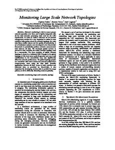
Figure 1: An arbitrary network topology. Each node represents a computer or a cluster of computers or a router. Each edge in the graph represents a direct link between two nodes. The topology here depicts �clusters� corresponding to local area networks or other subnetworks connected together via the network �backbone�. Broadly speaking, large scale network inference involves estimating network performance parameters based on tra�c measurements at a limited subset of the nodes. Y. Vardi was one of the �rst to rigorously study this sort of problem and coined the term network tomography [11] due to the similarity between network inference and medical tomography. Two forms of network tomography have been addressed in the recent literature: (i) link-level parameter estimation based on end-to-end, path-level tra�c measurements [12, 13, 14, 15, 16, 17, 18, 19, 20, 21] and (ii) sender-receiver path-level tra�c intensity estimation based on link-level tra�c measurements [22, 11, 23, 24, 25]. In link-level parameter estimation, the tra�c measurements typically consist of counts of packets transmitted and/or received between nodes or time delays between packet transmissions and receptions. The time delays are due to both propagation delays and router processing delays along the path. The measured path delay is the sum of the delays on the links comprising the path; the link delay comprises both the propagation delay on that link and the queueing delay 4
at the link's source node. A packet is dropped at a link if it does not successfully reach the input bu�er of the destination node. Link delays and occurrences of dropped packets are inherently random. Random link delays can be caused by router output bu�er delays, router packet servicing delays, and propagation delay variability. Dropped packets on a link are usually due to overload of the �nite output bu�er at the link's source node, but may also be caused by equipment downtime due to maintenance or power failures. Random link delays and packet losses become particularly signi�cant when there is a large amount of cross-tra�c competing for service by routers along a path. In path-level tra�c intensity estimation, the measurements consist of counts of packets that pass through nodes in the network. In privately owned networks, the collection of such measurements is relatively straightforward. Based on these measurements, the goal is to estimate how much tra�c originated from a speci�ed node and was destined for a speci�ed receiver. The combination of the tra�c intensities of all these origin-destination pairs forms the origindestination tra�c matrix. In this problem not only are the node-level measurements inherently random, but the parameter to be estimated (the origin-destination tra�c matrix) must itself be treated not as a �xed parameter but as a random vector. Randomness arises from the tra�c generation itself moreso than perturbations or measurement noise. The inherent randomness in both link-level and path-level measurements motivates the adoption of statistical methodologies for large scale network inference and tomography. Many network tomography problems can be roughly approximated by the (not necessarily Gaussian) linear model y = A� + �; (1) where: y is a vector of measurements, e.g. packet counts or end-to-end delays, taken at a number of di�erent measurement sites; A is a routing matrix; � is a vector of packet parameters, e.g. mean delays, logarithms of packet transmission probabilities over a link, or the random origin-destination tra�c vector. � is a noise term which can result from random perturbations of � about its mean value and possibly also additive noise in the measured data y; in the origindestination tra�c matrix estimation problem it is generally assumed to be zero. Typically, but not always, A is a binary matrix (the i; j -th element is equal to `1' or `0') that captures the topology of the network. The problem of large scale network inference refers to the problem of estimating the network parameters � given y and either a set of assumptions on the statistical distribution of the noise � or the introduction of some form of regularization to induce identi�ability. Speci�c examples are discussed below. What sets the large scale network inference problem (1) apart from other network inference problems is the potentially very large dimension of A which can range from a half a dozen rows and columns for a few packet parameters and a few measurement sites in a small local area network, to thousands or tens of thousands of rows and columns for a moderate number of parameters and measurements sites in the Internet. The associated high dimensional problems of estimating � are speci�c examples of inverse problems. Inverse problems have a very extensive literature both in signal processing [26], statistics [27], and in applied mathematics [28]. Solution methods for such inverse problems depend on the nature of the noise � and the A matrix and typically require iterative algorithms since they cannot be solved directly. In general, A is not of full-rank, so that identi�ability concerns arise. Either one must be content to resolve linear 5
combinations of the parameters or one must employ statistical means to introduce regularization and induce identi�ability. Both tactics are utilized in the examples in later sections of the paper. In most of the large scale Internet inference and tomography problems studied to date, the components of the noise vector � are assumed to be approximately independent Gaussian, Poisson, binomial or multinomial distributed. When the noise is Gaussian distributed with covariance independent of A� methods such as recursive linear least squares can be implemented using conjugate gradient, Gauss-Seidel, and other iterative equation solvers. When the noise is modeled as Poisson, binomial, or multinomial distributed more sophisticated statistical methods such as reweighted non-linear least squares, maximum likelihood via expectation-maximization (EM), and maximum a posteriori (MAP) via Monte Carlo Markov Chain (MCMC) algorithms can be used. These approaches will be illustrated in Sections 3 and 4.
2.1 Examples of Network Tomography Let us consider three concrete examples of the linear model (1). First, consider the problem of estimating the packet success probability on each link given end-to-end, source-to-destination (SD) counts of packet losses1 . Let � denote the collection of log success probabilities for each link. The SD log success probability is simply A�. Assuming a known number of packets sent from each source to destination, a binomial measurement model can be adopted [14]. When the number of packets sent and received are large, then the binomial model can be approximated with a Gaussian likelihood, leading to the classical linear model above (1). Second, suppose that endto-end, SR delays are measured and the goal is estimation of the delay probability distributions along each link. In this case, let � be a vector composed of the cumulant generating functions of the delay densities on each link. Then, with appropriate approximation arguments [20], y is again related to � according to the linear model (1). Third, in the origin-destimation (OD) tra�c matrix estimation case, y are link-level packet count measurements and � are the OD tra�c intensities. Gaussian assumptions are made on the origin-destination tra�c with a meanvariance relationship in high count situations in [17] leading to the linear equation (1) without the error term �. In each of these cases, the noise � may be correlated and have a covariance structure depending on A and/or �, leading to less than trivial inference problems. Moreover, in many cases the limited amount of data makes Gaussian approximations inappropriate and discrete observation models (e.g., binomial) may be more accurate descriptions of the discrete, packetized nature of the data. These discrete observation models necessitate more advanced inference tools such as the Expectation-Maximization algorithm and Monte Carlo simulation schemes (more on this in Section 3). Let us consider two further embellishments of the basic network inference problem described by the linear model (1). First, all quantities may, in general, be time-varying. For example, we may write y t = A t � t + �t ; (2) where t denotes time. The estimation problems now involve tracking time varying parameters. In fact, the time-varying scenario probably more accurately re�ects the dynamical nature of the true networks. There have been several e�orts aimed at tracking nonstationary network 1
The loss probabilities or �loss rates� are simply one minus the probability of successful transmission.
6
behavior which involve analogs of classical Kalman-�ltering methods [23, 15]. Another variation on the basic problem (1) is obtained by assuming that the routing matrix A is not known precisely. This leads to the so-called �topology discovery� problem [19, 29], and is somewhat akin to blind deconvolution or system identi�cation problems.
3 Link-Level Network Inference Link-level network tomography is the estimation of link-level network parameters (loss rates, delay distributions) from path-level measurements. Link-level parameters can be estimated from direct measurements when all nodes in a network are cooperative. Many promising tools such as pathchar (pchar), traceroute, clink, pipechar use Internet Control Message Protocol (ICMP) packets (control packets that request information from routers) in order to estimate linklevel loss, latencies and bandwidths. However, many routers do not respond to ICMP packets or treat them with very low priority, motivating the development of large-scale link-level network inference methods that do not rely on cooperation (or minimize cooperation requirements). In this article we discuss methods which require cooperation between a subset of the nodes in the network, most commonly the edge nodes (hosts or ingress/egress routers). Research to date has focused on the parameters of delay distributions, loss rates and bandwidths, but the general problem extends to the reconstruction of other parameters such as available bandwidths and service disciplines. The Multicast-based Inference of Network-internal Characteristics (MINC) Project at the University of Massachusetts [12] pioneered the use of multicast probing for network tomography, and stimulated much of the current work in this area [12, 13, 14, 30, 15, 16, 18, 19, 20, 31, 21]. We now outline a general framework for the link-level tomography problems considered in this section. Consider the scenario where packets are sent from a set of sources to a number of destinations. The end-to-end (path-level) behavior can be measured via a coordinated measurement scheme between the sender and the receivers. The sender can record whether a packet successfully reached its destination or was lost along the way and determine the transmission delay by way of some form of acknowledgement from the receiver to the sender upon successful packet reception. It is assumed that the senders cannot directly determine the speci�c link on which the packet was dropped nor measure delays or bandwidths on individual links within paths. A network can be logically represented by a graph consisting of r nodes connected by m links, labeled j = 1; : : : ; m. Potentially, a logical link connecting two nodes represents many routers and the physical links between them. Let there be n distinct measurement paths (from a sender to a receiver) through the network, labeled i = 1; : : : ; n. De�ne aij to be the probability that the i-th measurement path contains the j -th link. In most cases aij will take values (0; 1) but it is useful to maintain a level of generality which can handle random routing. A is the routing matrix having ij -th element aij . Figure 2 illustrates a simple network consisting of a single sender (node 0), two receivers (the leaves of the tree, nodes 2 and 3) and an internal node representing a router at which the 7
0
1
2
3
Figure 2: Tree-structured topology. two communication paths diverge (node 1). Only end-to-end measurements are possible, i.e., the paths are (0,2), and (0,3), where (s; t) denotes the path between nodes s and t. There are 3 links, and the matrix A has the form: ! 1 1 0 A= 1 0 1 (3) Note that in this example, A is not full rank. We discuss the rami�cations in later sections. A number of key assumptions underpin current link-level network tomography techniques, determining measurement frameworks and mathematical models. The routing matrix is usually assumed to be known and constant throughout the measurement period. Although the routing tables in the Internet are periodically updated, these changes occur at intervals of several minutes. However, the dynamics of the routing matrix may restrict the amount of data that can be collected and used for inference. Most current methodologies usually assume that that performance characteristics on each link are statistically independent of all other links, however this assumption is clearly violated due to common cross-tra�c �owing through the links. Assumptions of temporal stationarity are also made in many cases. In link-level delay tomography, it is generally assumed that synchronised clocks are available at all senders and receivers. Although many of the simplifying assumptions do not strictly hold, such ��rst-order� approximations have been shown to be reasonable enough for the large-scale inference problems of interest here. There are two modes of communication in networks: multicast and unicast. In unicast communication, each packet is sent to one and only one receiver. In multicast communication, the sender e�ectively sends each packet to a group of receivers. At internal routers where branching occurs, e.g., node 1 in Figure 2, each multicast packet is duplicated and sent along each branching path. We now overview the di�erent approaches to link-level network tomography that are enabled by the two modes of communication. Subsequently, we provide two detailed examples of link-level network tomography applications.
3.1 Multicast Network Tomography Network tomography based on multicast probing was one of the �rst approaches to the problem [13]. Consider loss rate tomography for the network depicted in Figure 2. If a multicast packet 8
is sent by the sender and received by node 2 but not by node 3, then it can be immediately determined that loss occurred on link 3 (successful reception at node 2 implies that the multicast packet reached the internal node 1). By performing such measurements repeatedly, the rate of loss on the two links 2 and 3 can be estimated; these estimates and the measurements enable the computation an estimate for the loss rate on link 1. To illustrate further, let �1 , �2 , and �3 denote the log success probabilities of the three links in the network, where the subscript denotes the lower node attached to the link. Let pb2j3 denote the ratio of the number of multicast packet probes simultaneously received at both nodes 2 and 3 relative to the total number received at node 3. This ratio provides a simple estimate of �2 . De�ne pb3j2 in a similar fashion and also let pbi , i = 2; 3, denote the ratio of the total number of packets received at node i over the total number of multicast probes sent to node i. We can then write
0 log pb 1 0 1 1 1 0 0� 1 BB log pb CC BB 1 0 1 CC B C (4) B@ log pb j CA � B@ 0 1 0 CA @ � A : � log pb j 0 0 1 A least squares estimate of f�i g is easily computed for this overdetermined system of equations. 2
1
3
2
23
3
32
Sophisticated and e�ective algorithms have been derived for large-scale network tomography in [13, 32]. Similar procedures can be conducted in the case of delay distribution tomography. There is a certain minimum propagation delay along each link, which is assumed known. Multicast a packet from node 0 to nodes 2 and 3, and measure the delay to each receiver. The delay on the �rst link from 0 to 1 is the identical for both receivers, and any discrepancy in the two end-toend delay measurements is solely due to a di�erence in the delay on link 1 to 2 and the delay link 1 to 3. This observation allows us to estimate the delay distributions on each individual link. For example, if the measured end-to-end delay to node 2 is equal to the known minimum propagation delay, then any extra delay to node 3 is incurred on link 1 to 3. Collecting delay measurements from repeated experiments in which the end-to-end delay to node 2 is minimal allows construction of a histogram estimate of the delay distribution on link 1 to 3. In larger and more general trees, the estimation becomes more complicated. Advanced algorithms have been developed for multicast-based delay distribution tomography on arbitrary tree-structured networks [18, 32].
3.2 Unicast Network Tomography Alternatively, one can tackle loss rate and delay distribution tomography using unicast measurements. Unicast measurements are more di�cult to work with than multicast, but since many networks do not support multicast, unicast-based tomography is of considerable practical interest. The di�culty of unicast-based tomography is that although single unicast packet measurements allow one to estimate end-to-end path loss rates and delay distributions, there is not a unique mapping of these path-level parameters to the corresponding individual link-by-link parameters. For example, referring again to Figure 2, if packets are sent from node 0 to nodes 2 and 3 and nk and mk denote the numbers of packets sent to and received by receiver node k, 9
k = 2; 3, then
log pb2 log pb3
!
!0 � 1 � 11 10 01 B @ � CA | {z } � 1 2
A
(5)
3
where pbk = mk =nk and �j , j = 1; 2; 3 denotes the log success probability associated with each link. Clearly, a unique solution for f�j g does not exist since A is not full rank. To address this challenge in unicast loss tomography, the authors of [14] and [17] independently proposed methodologies based on measurements made using unicast, back-to-back packet pairs. These measurements provide an opportunity to collect more informative statistics that can help to resolve the link-level loss rates and delay distributions. A packet pair describes two packets that are sent one after the other by the sender, possibly destined for di�erent receivers, but sharing a common set of links in their paths. In networks whose queues obey a droptail policy2 , if two back-to-back packets are sent across a common link and one of the pair is sucessfully transmitted across the link, then it is highly probable that the other packet is also successful. Similarly, the two packets in each pair will experience roughly the same delay through shared links. These observations has been veri�ed experimentally in real networks [34, 16]. If one assumes that the probability of success for one packet conditional on the success of the other is approximately unity, then the same methodology developed for multicast-based tomography (as described above) can be employed with unicast, packet-pair measurements [16]. In the case of bandwidth tomography, the authors of [35] addressed the challenge of nonuniqueness through clever use of the header �elds of unicast packets. The time-to-live (TTL) �eld in each packet header indicates how many hops the packet should traverse. At each router the packet encounters, the TTL counter is decremented by one; when the counter reaches zero, the next router discards the packet. The nettimer program described in [35] uses �tailgating� to collect measurements: many packet-pairs are sent from the source, each consisting of a large packet followed by a small packet. The TTL �eld of the large packet is varied during the measurement period so that it is propagated through only a portion of the path. The endto-end delay measured by the small packet (in a relatively uncongested network) is primarily comprised of the propagation delay experienced by the large packet, enabling inference of the bandwidth of the subpath traversed by the large packet. Referring to the simple triad network in Figure 2 for illustration, nettimer might send packet-pairs form node 0 along path 0-1-2. If the TTL of the large packet is set to one, the tailgating smaller packet measures the propagation delay on link 0-1. Unicast measurement can be conducted either actively or passively. In the case of active measurement, probe packets are sent by the senders speci�cally for the purpose of estimation. In passive monitoring, the sender extracts data from existing communications (e.g., records of TCP sessions). Loss rate and delay distribution tomography methods have been developed speci�cally for unicast packet pairs in [14, 17, 36, 37]. Unicast packet stripes (triples, quadruples, etc.) have also been investigated for loss rate tomography [16]. A droptail queueing policy means that a packet is dropped by a queue only if it reaches the queue and there is insu�cient space in the bu�er. In active queueing strategies, such as random-early-detection (RED) [33], packets can be dropped even if they have already entered the queue 2
10
3.3 Example: Unicast Inference of Link Loss Rates Link loss rates can be inferred from end-to-end, path-level unicast packet measurements using the approximate linear model given in equations (1) when the numbers packet counts are large; refer to Section 3.2. However, as stated earlier the discrete process of counting the number of sent and received packets suggests the use of a discrete probability distribution in our modeling and analysis. We give a brief introduction and example of this approach here, and for more details the interested reader is referred to related papers [14, 15]. The successful traversal of a single packets across a link can be reasonably modeled as a sequence of Bernoulli events. Associate with the j-th link in the network a single parameter governing the Bernoulli model. This parameter is the probability (rate) of successful transmission on the link �j . The complete set �j ; j 2 1; : : : ; m form the success rates that network loss tomography strives to identify. Measurements are collected by sending nk single packets along the path to receiver k and recording how many successfully reached the destination, denoted as mk . Determination of the success of a given packet is handled by an acknowledgement sent from the receiver back to the sender. For example, such acknowledgements are a built-in feature of TCP. The likelihood of mk given nk is binomial (since Bernoulli losses are assumed) and is given by
l(mk j nk ; pk ) =
Q
!
nk pmk (1 , p )nk ,mk ; k mk k
(6)
where pk = j 2P (0;k) �j and P (0; k) denotes the sequence of nodes in the path from the sender 0 to receiver k. If the routing matrix A is full rank, then unique maximum likelihood estimates of the loss rates can be formed by solving a set of linear equations. If A is not full rank, then there is no unique mapping of the path success probabilities to the success probabilities on individual links (between routers) in the path. To overcome this di�culty, measurements are made using back-to-back packet pairs or sequences of packets as discussed above [14, 17, 16]. If two, back-to-back packets are sent to node j from its parent node �(j ), then de�ne the conditional success probability as
i � Pr(1st packet �(j ) ! j j 2nd packet �(j ) ! j ); where �(j ) ! j is shorthand notation denoting the successful transmission of a packet from �(j ) to j . That is, given that the second packet of the pair is received, then the �rst packet is received with probability j and dropped with probability 1 , j . It is anticipated that j � 1 for each j , since knowledge that the second packet was successfully received suggests that the queue for link j was not full when the �rst packet arrived. Evidence for such behavior has been provided by observations of the Internet [38, 34]. Suppose that each sender sends a large number of back-to-back packet pairs in which the �rst packet is destined for one of its receivers k and the second for another of its receivers l. The time between pairs of packets must be considerably larger than the time between two packets 11
in each pair. Let nk;l denote the number of pairs for which the second packet is successfully received at node l, and let mk;l denote the number of pairs for which both the �rst and second packets are received at their destinations. With this notation, the likelihood of mk;l given nk;l is binomial and is given by
l(mk;l j nk;l; pk;l) =
!
nk;l pmk;l (1 , p )nk;l ,mk;l ; k;l mk;l k;l
where pk;l is a product whose factors are elements on the shared links and � elements on the unshared links. The overall likelihood function is given by
l(mjn; p) �
Y k
l(mk jnk ; pk ) �
Y k;l
l(mk;l jnk;l ; pk;l )
(7)
The goal is to determine the vectors � and that maximize (7). Maximizing the likelihood function is not a simple task because the individual likelihood functions l(mk j nk ; pk ) or l(mk;l j nk;l ; pk;l ) involve products of the and/or � probabilities. Consequently, numerical optimization strategies are required. The Expectation-Maximization (EM) algorithm is an especially attractive option that o�ers a stable, scalable procedure whose complexity grows linearly with network dimension [14]. The link-level loss inference framework is evaluated in [37] using the ns-2 network simulation environment [39]. Measurements were collected by passively monitoring existing TCP connections3 . The experiments involved simulation of the 12-node network topology shown in Figure 1. This topology re�ects the nature of many networks � a slower entry link from the sender, a fast internal backbone, and then slower exit links to the receivers. In the simulations, numerous short-lived TCP connections were established between the source (node 0) and the receivers (nodes 5-11). In addition, there is cross-tra�c on internal links, such that in total there are approximately thirty TCP connections and thirty User Datagram Protocol (UDP)4 connections operating within the network at any one time. The average utilisation of the network is in all cases relatively high; otherwise, few packet drops occur and loss estimation is of little interest. All the TCP connections �owing from the sender to the receivers are used when collecting packet and packet-pair measurements (see [37] for details on the data collection process). Measurements were collected over a 300 second interval. The experiments were designed to ascertain whether the unicast link-level loss tomography framework is capable of discerning where signi�cant losses are occurring within the network. They assess its ability to determine how extensive the heavy losses are and to provide accurate estimates of loss rates on the better performing links. Three tra�c scenarios were explored. In Scenario 1, links 1-2 and 2-5 experience substantial losses, thereby testing the framework's ability to separate cascaded losses. In Scenario 2, links 1-2 and 4-8 experience substantial loss, Data transmission in the Internet is primarily handled by the Transmission Control Protocol (TCP) and Internet Protocol (IP). TCP/IP were developed by a Department of Defense to allow cooperating computers to share resources across a network. IP is responsible for moving packets of data from node to node and TCP coordinates the delivery between the sender and receiver (server and client). 4 UDP is a simpler protocol than TCP. UDP simply sends packets and does not receive an acknowledgement from the receiver. 3
12
(testing the ability to resolve distributed losses in di�erent branches of the network). In Scenario 3, many more on-o� UDP and on-o� TCP connections were introduced throughout the topology. Figure 3 displays the simulation results for each of the di�erent tra�c scenarios.
3.4 Example: Unicast Inference of Link Delay Distributions When the link delays along a path are statistically independent the end-to-end delay densities are related to the link delay densities through a convolution. Several methods for unraveling this convolution from the end-to-end densities are: 1) transformation of the convolution into a more tractable matrix operator via discretization of the delays [18, 15, 20]; estimation of low order moments such as link delay variance [32] from end-to-end delay variances which are additive over the probe paths; 3) estimation of the link delay cumulant generating functions (CGF) [20, 31] from the end-to-end delay CGF's which are also additive over the probe paths. Here we discuss the CGF estimation method from which any set of delay moments can be recovered. Let Yi denote the total end-to-end delay of a probe sent along the i-th probe path. Then
Yi = ai1 Xi1 + � � � + aim Xim ;
i = 1; : : : n
(8)
where Xij is the delay of the i-th probe along the j -th link in the path and aij 2 f0; 1g are elements of the routing matrix A. Here fXij gni=1 are assumed to be i.i.d. realizations of a random variable Xj associated with the delay of the j -th link. The CGF of a random variable Y is de�ned as KY (t) = log E [etY ] where t is a variable which can be real or complex depending on the application. When Y is a sum of a set fXj gmj=1 of independent random variables the CGF satis�es the additive property KY (t) = Pmstatistically j =1 KXj (t). Therefore, in view of the end-to-end delay representation (8), and assuming independent Xi1 ; : : : ; Xim (spatial independence), the vector of CGFs of the end-to-end probe delays fYi gmi=1 of the i-th probe satis�es the linear system of equations
KY (t) = A � KX (t); where KY (t) = [KY (t); : : : ; KYn (t)]T and KX (t) = [KX (t); : : : ; KXm (t)]T 1
m-element vector functions of t, respectively.
1
(9) are n-element and
The linear equation (9) raises two issues of interest: 1) conditions on A for identi�ability of KX (t) from KY (t); and 2) good methods of estimation of KX (t) from end-to-end delay measurements Yi , i = 1; : : : ; n. When A is not full rank, only linear combinations of those link CGFs lying outside of the null space of A can be determined from (9). We call such a linear combination an identi�able subspace of CGFs. Depending P on the routing matrix A, identi�able subspaces can correspond to weighted averages of CGFs Nj=1 �j KXj (t) over a region of the network. This motivates a multi-resolution successive re�nement algorithm for detecting and isolating bottlenecks, faults, or other spatially localized anomalies. In such an algorithm large partially overlapping regions of the network are probed with a small number of probes just su�cient for each of the CGF linear combinations to be sensitive to anomalous behavior of the aggregate regional delay distributions. 13
1 0.95
0
1Mb /s
True prob Est. prob
0.9
1
1
1Mb /s
3Mb /s 0.95
2
0.9
2Mb /s 0.66Mb /s
6
7
8
0.02
0.8Mb /s
4
0.92Mb /s 1Mb /s
5
True prob Est. prob
3
1Mb /s
1Mb /s 9
1Mb /s 10
DropTail RED
0.01
11
0 1
3
5
7
9
(a) A network consisting of a single sender (node 0), four internal routers (nodes 1-4), and seven receivers (nodes 5-11). The bandwidth in megabits/second (Mb/s) is indicated for each link.
(b) Scenario 1: Heavy losses on links 2 and 5
1
1
0.9
0.95
True prob Est. prob
0.8
0.9
1
1
0.9 0.8
True prob Est. prob
0.9
0.02
DropTail RED
DropTail RED
0.02
0.01 0 1
True prob Est. prob
0.95
True prob Est. prob
11
0.01 3
5
7
9
0 1
11
(c) Scenario 2: Heavy losses on links 2 and 8
3
5
7
9
11
(d) Scenario 3: Tra�c mixture medium losses
Figure 3: Performance of the link-level loss tomography framework examined through ns-2 simulation of the network in (a). Panels (b)-(d) show true and estimated link-level success rates of TCP �ows from the source to receivers for several tra�c scenarios, as labeled above. In (b)-(d), the two panels display for each link 1-11 (horizontal axis): (top) an example of true and estimated success rates and (bottom) mean absolute error between estimated and true success rates over 10 trials.
14
If one of the regions was identi�ed as a potential site of anomalous behavior a similar probing process is repeated on subregions of the suspected region. This process continues down to the single link level within a small region and requires substantially fewer probe paths than would be needed to identify the set of all link delay CGF's. Estimation of the CGF vector KX (t) from an i.i.d. sequence of end-to-end probe delay experiments can be formulated as solving a least squares problem in a linear model analogous to (1): K^ Y (t) = A � KX (t) + �(t): (10) ^ Y is an empirical estimate of the end-to-end CGF vector and � is a residual error. where K Di�erent methods of solving for KX result by assuming di�erent models for the statistical distribution of the error residual. One model, discussed in [20], is obtained by using a methodof-moments (MOM) estimator for KY and invoking the property that MOM estimators are asymptotically Gaussian distributed as the number of experiments gets large. The bias and ^ Y can then be approximated via bootstrap techniques and an approximate covariance of K maximum likelihood estimate of KX is generated by solving (10) using iteratively reweighted least squares (LS). Using other types of estimators of KY , e.g. kernel based density estimation or mixture models with known or approximatable bias and covariance, would lead to di�erent LS solutions for KX . The ns-2 network simulator was used to perform a simulation of the 4 link network shown in Figure 4. All four links had ns-2 bandwidth set equal to 4Mb/sec and latency set equal
Probe 5
Link 2
Link 1 Probe 1 Probe 2 Probe 3
Link 3
Probe 4
Link 4
Figure 4: Unicast delay estimation probe routing used in ns-2 simulation. Tailgating can be used to emulate the internal probes 3,4,5.
to 50ms. Each link was modeled as a Drop-Tail queue (FIFO queue with �nite bu�er) with queue bu�er size of 50 packets. Probes were generated as 40 byte UDP packets at each sender node according to a Poisson process with mean interarrival time being 16ms and rate 20Kb/sec. The background tra�c consisted of both Exponential on-o� UDP tra�c and FTP tra�c. The background tra�c on link 3 was approximatly 10 times higher than the background tra�c on the other links to simulate a �bottleneck� link. R Table 1 shows the integrated mean squared error 01 jKXj (t) , K^ Xj (t)j2 dt based on LS estimators with bootstrap bias correction (�rst row) and no bias correction (row 2). 15
Table 1: MSE of K^ Xj (bias correction) and K^ X0 j (no bias correction) for estimated link CGF's. Link 1 2 3 4 ^ MSE of KXj 0.00033 0.00013 0.00045 0.00013 MSE of K^ X0 j 0.00031 0.00015 0.00132 0.00017 We next illustrate the application of the CGF technique to bottleneck detection. De�ne a bottleneck as the event that a link delay exceeds a speci�ed delay threshold. The Cherno� bound speci�es an upper bound on the probability of bottleneck in the j -th link in terms of the CGF � � P (Xj � �) � min e,t� etKXj (t) : (11) t>0
In Table 2, we show the Cherno� bound Pj on the bottleneck probability P (Xj � � = 0:02s) (s denotes �seconds") which were estimated by plugging bias corrected CGF estimates into the right hand side of (11). Also shown are the �true� link exceedance probabilities which were empirically estimated from directly measured single-link loss statistics from an independent ns-2 simulation. Note that while the Cherno� bounds are sometimes greater than one, the amplitude of the bound follows the trend of the true bottleneck probabilities. In particular if we set as our criterion for detection of a bottleneck as: �the probability that Xj exceeds 0:02s is at least 0:95", we see that the estimated Cherno� bound correctly identi�es link 3 as the bottleneck link. Table 2: Cherno� bound Pj and empirical estimate of P (Xj � 0:02). A bottleneck at link 3 is correctly identi�ed if one selects a 95 percentile bottleneck detection level (Pj � 0:95). Link 1 2 3 4 Pj 0.9424 0.9295 1.0025 0.9329 P (Xj � �) 0.0014 0.0002 0.9932 0.0003
4 Origin-Destination Tomography Origin-destination tomography is essentially the antithesis of link-level network tomography: the goal is the estimation of path-level network parameters from measurements made on individual links. By far the most intensively studied origin-destination network tomography problem is the estimation of origin-destination (OD) tra�c from measurable tra�c at router interfaces. In privately-owned networks, the collection of link tra�c statistics at routers within the network is often a far simpler task than performing direct measurement of OD tra�c. The OD tra�c matrix, which indicates the intensity of tra�c between all origin-destination pairs in a network, is a key input to any routing algorithm, since the link weights of the Open Shortest Path First5 Open Shortest Path First (OSPF) is a routing protocol developed for IP networks. OSPF is a link-state routing protocol that calls for the sending of link-state advertisements to all other routers in the same hierarchical area. A link state takes the form of a weight, e�ectively the cost of routing via that link. 5
16
(OSPF) routing protocol are related to the tra�c on the paths. Ideally, a data-driven OD matrix should be central to the routing optimization program. There are currently two ways to obtain OD tra�c counts. Indirect methods are considered in [11, 22, 25, 23]; a direct method via software such as NetFlow supported by Cisco routers is described in [23, 40]. Both approaches need the cooperation of the routers in the network, but this is not problematic for privately-owned networks. The link tra�c counts at routers are much easier to collect relative to the direct approach via NetFlow and lead to a linear inverse problem. There are noticeable features about this particular inverse problem worthy of elaboration. Firstly, the OD tra�c vector to be estimated is not a �xed parameter vector, but a random vector, denoted by x; secondly, the linear equation (1) is used without the error term � (stochastic variability is captured in x); thirdly, even though A is singular as in other cases discussed, these techniques use statistical means to induce a regularization enabling the recovery of the whole x (or the tra�c intensities underlying x). Moreover, the most recent work [23] on this also deals with the time-varying aspect of the data. Vardi was the �rst to investigate this problem. In [11] he studies a network with a general topology, using an iid Poisson model for the OD tra�c byte counts. He speci�es identi�ability conditions under the Poisson model and develops a method that uses the EM algorithm on link data to estimate Poisson parameters in both deterministic and Markov routing schemes. To mitigate the di�culty in implementing the EM algorithm under the Poisson model, he proposes a moment method for estimation and brie�y discusses the normal model as an approximation to the Poisson. Related work treated the special case involving a single set of link counts and also employed an EM algorithm [25]. A Bayesian formulation and Markov Chain Monte Carlo estimation technique has also been proposed [22]. Cao et al. [23] use real data to revise the Poisson model and to address the non-stationary aspect of the problem. Their methodology is validated through comparison with direct (but expensive) collection of OD tra�c. Cao et al. represent link count measurements as summations of various OD counts that were modeled as independent random variables. (Even though Tra�c Control Protocol (TCP) feedback creates dependence, direct measurements of OD tra�c indicate that the dependence between tra�c in opposite directions is weak. This renders the independence assumption a reasonable approximation.) Time-varying tra�c matrices estimated from a sequence of link counts were validated on a small subnetwork with 4 origins/destinations by comparing the estimates with actual OD counts that were collected by running Cisco's NetFlow software on the routers. Such direct point-to-point measurements are often not available because they require additional router CPU resources, can reduce packet forwarding e�ciency, and involve a signi�cant administrative burden when used on a large scale. Let y = (y1 ; : : : ; ym )T denote the observed column vector of incoming/outgoing byte counts measured on each router link interface during a given time interval and let x = (x1 ; : : : ; xn )T denote the unobserved vector of corresponding byte counts for all OD pairs in the network. Here T indicates transpose and x is the `tra�c matrix' even though it is arranged as a column vector for convenience. One element of x, for example, corresponds to the number of bytes originating from a speci�ed origin node to a speci�ed destination node, whereas one element of y corresponds to bytes sent from the origin node regardless of their destination. Thus each 17
element of y is a sum of selected elements of x, so
y = Ax
(12)
xi � normal(�i ; ��i ); independently
(13)
y � normal(A�; A�A0);
(14)
where A is a m � n routing matrix of 0's and 1's that is determined by the routing scheme of the network. The work of [23] only considers �xed routing, i.e. there is only one route from an origin to a destination. In [23] the unobserved OD byte counts are modeled as and this implies where
� = (�1 ; : : : ; �n )0 ; and � = � diag(�c1 ; : : : ; �cn ):
Here � > 0 s the vector of OD mean rates and c is a �xed power constant (both c = 1 and 2 work well with the Lucent network data as shown in [23, 24]). � > 0 is a scale parameter that relates the variance of the counts to their mean, since usually larger counts have larger variance. The mean-variance relationship is necessary to ensure the identi�ability of the parameters in the model. Heuristically, under this constraint, the covariances between the y's give the identi�ability of the parameters up to the scale parameter � which can be determined from the expectation of a y. Cao et al. [23] address the non-stationarity in the data using a local likelihood model (cf. [41]); that is, for any given time t, analysis is based on a likelihood function derived from the observations within a symmetric window of size w around t (e.g., in the experiments described below, w = 11 corresponds to observations within about an hour in real time). Within this window, an iid assumption is imposed (as a simpli�ed and yet practical way to treat the approximately stationary observations within the window). And maximum-likelihood estimation is carried out for the parameter estimation via a combination of the EM algorithm and a second-order global optimization routine. The component-wise conditional expectations of the OD tra�c, given the link tra�c, estimated parameters, and the positivity constraints on the OD tra�c, are used as the initial estimates of the OD tra�c. The linear equation y = Ax is enforced via the iterative proportional �tting algorithm (cf. [42, 43]) to obtain the �nal estimates of the OD tra�c. The positivity and the linear constraints are very important �nal steps to get reliable estimates of the OD tra�c, in addition to the implicit regularization introduced by the iid statistical model. To smooth the parameter estimates, a random walk model is applied to the logarithm of the parameters �'s and � over the time windows.
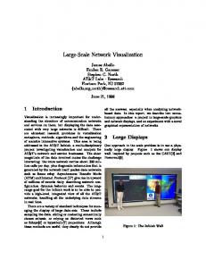
4.1 Example: Time-varying OD Tra�c Matrix Estimation Figure 5 is a network at Lucent Technologies considered in [23, 24]. Figures 6 and 7 are taken from [23]. They show the validation (via NetFlow) and estimated OD tra�c based on the link tra�c for the subnetwork around Router 1 with 4 origins/destinations in Figure 5. Figure 6 gives the full scale and Figure 7 is the zoomed-in scale (20�). It is obvious that the estimated 18
OD tra�c agrees well with the NetFlow measured OD tra�c for large measurements, but not so well for small measurements where the Gaussian model is a poor approximation. From the point of view of tra�c engineering, it is adequate that the large tra�c �ows are inferred accurately. Hence for some purposes such as planning and provisioning activities estimates of OD tra�c could be used as inexpensive substitutes for direct measurements. Firewall
fddi local corp
Router1 Router2
Gateway
Router3 Router4
internet
Switch
Router5
Figure 5: A network at Lucent Technologies Even though the method described in [23] uses all available information to estimate parameter values and the OD tra�c vector x, it does not scale to networks with many nodes. In general, if there are Ne edge nodes, the number of �oating point operations needed to compute the MLE is at least proportional to Ne5 . A scalable algorithm that relies on a divide-and-conquer strategy to lower the computational cost without losing much of the estimation e�ciency is proposed in [24].
5 Conclusion and Future Directions This paper has provided an overview of the emerging area of large scale inference and tomography in communications networks. Statistical signal processing will continue to play an important role in this area and here we attempt to stimulate the reader with an outline of some of the many open issues. These issues can be divided into extensions of the theory and potential networking applications areas. The spatio-temporally stationary and independent tra�c and network transport model has limitations, especially in tomographic applications involving heavily loaded networks. Since one of the principal applications of network tomography is to detect heavily loaded links and subnets relaxation of these assumptions continues to be of great interest. Some recent work on relaxing spatial dependence and temporal independence has appeared in unicast [20] and multicast [13] settings. However, we are far from the point of being able to implement �exible yet tractable models which simultaneously account for long time tra�c dependence, latency, dynamic random routing, and spatial dependence. As wireless links and ad hoc networks become more prevalent spatial dependence and routing dynamics will become dominant. Recently, there have been some preliminary attempts to deal with the time-varying, nonsta19
tionary nature of network behavior. In addition to the estimation of time-varying OD tra�c matrices discussed in Section 4, others have adopted a dynamical systems approach to handle nonstationary link-level tomography problems [36]. Sequential Monte Carlo inference techniques are employed in [36] to track time-varying link delay distributions in nonstationary networks. One common source of temporal variability in link-level performance is the nonstationary characteristics of cross-tra�c. Figure 8 illustrates this scenario and displays the estimated delay distributions at di�erent time instances (see [36] for further details). There is also an accelerating trend toward network security will create a highly uncooperative environment for active probing � �rewalls designed to protect information may not honor requests for routing information, special packet handling (multicast, TTL, etc), and other network transport protocols required by many current probing techniques. This has prompted investigations into more passive tra�c monitoring techniques, for example based on sampling TCP tra�c streams [37]. Furthermore, the ultimate goal of carrying out network tomography on a massive scale poses a signi�cant computational challenge. Decentralized processing and data fusion will probably play an important role in reducing both the computational burden and the high communications overhead of centralized data collection from edge-nodes. The majority of work reported to date has focused on reconstruction of network parameters which may only be indirectly related to the decision-making objectives of the end-user regarding the existence of anomalous network conditions. An example of this is bottleneck detection which has been considered in [31, 21] as an application of reconstructed delay or loss estimation. However, systematic development of large scale hypothesis testing theory for networks would undoubtedly lead to superior detection performance. Other important decision-oriented applications may be detection of coordinated attacks on network resources, network fault detection, and veri�cation of service. Finally the impact of network monitoring, which is the subject of this article, on network control and provisioning could become the application area of most practical importance. Admission control, �ow control, service level veri�cation, service discovery, and e�cient routing could all bene�t from up-to-date and reliable information about link and router level performances. The big question is: can signal processing methods be developed which ensure accurate, robust and tractable monitoring for the development and administration of the Internet and future networks?
References [1] RTP: A transport protocol for real-time applications, Jan. 1996. IETF Internet Request For Comments: RFC 1889. [2] N. Du�eld and M. Grossglauser. Trajectory sampling for direct tra�c observation. In Proc. ACM SIGCOMM 2000, Stockholm, Sweden, Aug. 2000. [3] F. P. Kelly, S. Zachary, and I. Ziedins. Stochastic networks: theory and applications. Royal Statistical Society Lecture Note Series. Oxford Science Publications, Oxford, 1996. 20
[4] X. Chao, M. Miyazawa, and M. Pinedo. Queueing networks: customers, signals and product form solutions. Systems and Optimization. Wiley, New York, NY, 1999. [5] W. Leland, M. Taqqu, W. Willinger, and D. Wilson. On the self-similar nature of Ethernet tra�c (extended version). IEEE/ACM Trans. Networking, pages 1�15, 1994. [6] V. Paxson. End-to-end internet packet dynamics. In Proc. ACM SIGCOMM, 1997. [7] R. Riedi, M. S. Crouse, V. Ribeiro, and R. G. Baraniuk. A multifractal wavelet model with application to TCP network tra�c. IEEE Trans. Info. Theory, Special issue on multiscale statistical signal analysis and its applications, 45:992�1018, April 1999. [8] A. Feldmann, A. C. Gilbert, P. Huang, and W. Willinger. Dynamics of IP tra�c: a study of the role of variability and the impact of control. In Proc. ACM SIGCOMM, pages 301�313, Cambridge, MA, 1999. [9] A. C. Gilbert, W. Willinger, and A. Feldmann. Scaling analysis of conservative cascades, with applications to network tra�c. IEEE Trans. Info. Theory, IT-45(3):971�991, Mar. 1999. [10] A. Veres, Z. Kenesi, S. Molnár, and G. Vattay. On the propagation of long-range dependence in the Internet. In Proc. ACM SIGCOMM 2000, Stockholm, Sweden, Aug. 2000. [11] Y. Vardi. Network tomography: estimating source-destination tra�c intensities from link data. J. Amer. Stat. Assoc., pages 365�377, 1996. [12] Multicast-based inference of network-internal characteristics (MINC). http://gaia.cs.umass.edu/minc. [13] R. Cáceres, N. Du�eld, J. Horowitz, and D. Towsley. Multicast-based inference of networkinternal loss characteristics. IEEE Trans. Info. Theory, 45(7):2462�2480, November 1999. [14] M. Coates and R. Nowak. Network loss inference using unicast end-to-end measurement. In ITC Seminar on IP Tra�c, Measurement and Modelling, Monterey, CA, Sep. 2000. [15] M. Coates and R. Nowak. Network delay distribution inference from end-to-end unicast measurement. In Proc. IEEE Int. Conf. Acoust., Speech, and Signal Proc., May 2001. [16] N.G. Du�eld, F. Lo Presti, V. Paxson, and D. Towsley. Inferring link loss using striped unicast probes. In Proceedings of IEEE INFOCOM 2001, Anchorage, Alaska, April 2001. [17] A. Bestavros K. Harfoush and J. Byers. Robust identi�cation of shared losses using endto-end unicast probes. In Proc. IEEE Int. Conf. Network Protocols, Osaka, Japan, Nov. 2000. Errata available as Boston University CS Technical Report 2001-001. [18] F. Lo Presti, N.G. Du�eld, J. Horowitz, and D. Towsley. Multicast-based inference of network-internal delay distributions. Technical report, University of Massachusetts, 1999. [19] S. Ratnasamy and S. McCanne. Inference of multicast routing trees and bottleneck bandwidths using end-to-end measurements. In Proceedings of IEEE INFOCOM 1999, New York, NY, March 1999. 21
[20] M.F. Shih and A.O. Hero. Unicast inference of network link delay distributions from edge measurements. Technical report, Comm. and Sig. Proc. Lab. (CSPL), Dept. EECS, University of Michigan, Ann Arbor, May 2001. [21] A.-G. Ziotopolous, A.O. Hero, and K. Wasserman. Estimation of network link loss rates via chaining in multicast trees. In Proc. IEEE Int. Conf. Acoust., Speech, and Signal Proc., May 2001. [22] C. Tebaldi and M. West. Bayesian inference on network tra�c using link count data (with discussion). J. Amer. Stat. Assoc., pages 557�576, June 1998. [23] J. Cao, D. Davis, S. Vander Wiel, and B. Yu. Time-varying network tomography: router link data. J. Amer. Statist. Assoc, 95:1063�1075, 2000. [24] J. Cao, S. Vander Wiel, B. Yu, and Z. Zhu. A scalable method for estimating network tra�c matrices from link counts. URL: http://www.stat.berkeley.edu/�binyu/publications.html, 2000. [25] R.J. Vanderbei and J. Iannone. An EM approach to OD matrix estimation. Technical Report SOR 94-04, Princeton University, 1994. [26] R. J. Mammone. Inverse problems and signal processing. In The Digital Signal Processing Handbook, chapter VII. CRC Press, Boca Raton, FL, 1998. [27] Finbarr O'Sullivan. A statistical perspective on ill-posed inverse problems. Statistical Science., 1(4):502�527, 1986. [28] F. Natterer. The Mathematics of Computerized Tomography. Wiley, New York, 1986. [29] R. Cáceres, N. Du�eld, J. Horowitz, F. Lo Presti, and D. Towsley. Loss-based inference of multicast network topology. In Proc. IEEE Conf. Decision and Control, Dec. 1999. [30] M. Coates and R. Nowak. Networks for networks: Internet analysis using Bayesian graphical models. In IEEE Neural Network for Signal Processing Workshop, Sydney, Aust., Dec. 2000. [31] M.F. Shih and A.O. Hero. Unicast inference of network link delay distributions from edge measurements. In Proc. IEEE Int. Conf. Acoust., Speech, and Signal Proc., May 2001. [32] N. Du�eld and F. Lo Presti. Multicast inference of packet delay variance at interior network links. In Proceedings of IEEE INFOCOM 2000, Tel Aviv, Israel, Mar. 2000. [33] Recommendations on queue management and congestion avoidance in the Internet, Apr. 1998. IETF Internet Request For Comments: RFC 2309. [34] V. Paxson. End-to-end Internet packet dynamics. IEEE/ACM Trans. Networking, 7(3):277�292, June 1999. [35] K. Lai and M. Baker. Measuring link bandwidths using a deterministic model of packet delay. In Proc. ACM SIGCOMM 2000, Stockholm, Sweden, Aug. 2000. 22
[36] M. Coates and R. Nowak. Sequential Monte Carlo inference of internal delays in nonstationary communication networks. to appear in IEEE Trans. Signal Processing, Special Issue on Monte Carlo Methods for Statistical Signal Processing, 2001. [37] Y. Tsang, M. Coates, and R. Nowak. Passive network tomography using EM algorithms. In Proc. IEEE Int. Conf. Acoust., Speech, and Signal Proc., May 2001. [38] J-C. Bolot. End-to-end packet delay and loss behaviour in the Internet. In Proc. ACM SIGCOMM 1993, pages 289�298, Sept. 1993. [39] UCB/LBNL/VINT network simulator ns (version 2). URL: http://www.isi.edu/nsnam/ns/. [40] A. Feldmann, A. Greenberg, C. Lund, N. Reingold, J. Rexford, and F. True. Deriving tra�c demands for operational IP networks: methodology and experience. In Proc. ACM SIGCOMM 2000, Stockholm, Sweden, Aug. 2000. [41] C. Loader. Local regression and likelihood. Springer, New York, NY, 1999. [42] W. E. Deming and F. F. Stephen. On a least squares adjustment of a sampled frequency table when the expected marginal totals are known. Ann. Math. Statist., 11:427�444. [43] I. Csiszár. I-divergence geometry of probability distributions and minimization problems. Ann. Probab., 3(1):146�158, 1975.
23
Xhat 0
4
8
12
16
20
X 24
0
4
8
12
16
20
24
dst fddi
dst switch
dst local
dst corp
total
corp->fddi
corp->switch
corp->local
corp->corp
ori corp
1M 800K 600K 400K 200K 0
1M 800K 600K 400K 200K
bytes/sec
0 local->fddi
local->switch
local->local
local->corp
ori local
switch->fddi
switch->switch
switch->local
switch->corp
ori switch
1M 800K 600K 400K 200K 0 1M 800K 600K 400K 200K 0 fddi->fddi
fddi->switch
fddi->local
fddi->corp
ori fddi
1M 800K 600K 400K 200K 0 0
4
8
12
16
20
24
0
4
8
12
16
20
24
0
4
8
12
16
hour of day
Figure 6: Full-scale time series plots of OD tra�c on Feb. 22, 1999 for Router 1 sub-network with 4 origins/destinations. In the lower-left 4�4 matrix, the rows (from TOP down) correspond to corp, local, switch and fddi and the columns (from RIGHT to LEFT) correspond to corp, local, switch and fddi. These 4 � 4 main panels correspond to the 16 OD pairs. For example, the (1,2) panel is corp ! switch. The 8 marginal panels (above and to the right of the main matrix) are the observed link tra�c used to infer the 16 OD tra�c pairs. The top-right corner shows the total observed link tra�c. Xhat is the estimated OD tra�c and X is the observed OD tra�c. At this time-scale it is impossible to di�erentiate between estimated and observed OD tra�c in most panels of the matrix.
24
20
24
Xhat 0
4
8
12
16
20
X 24
0
4
8
12
16
20
24
dst fddi
dst switch
dst local
dst corp
total
corp->fddi
corp->switch
corp->local
corp->corp
ori corp
50K 40K 30K 20K 10K 0
50K 40K 30K 20K 10K
bytes/sec
0 local->fddi
local->switch
local->local
local->corp
ori local
switch->fddi
switch->switch
switch->local
switch->corp
ori switch
50K 40K 30K 20K 10K 0 50K 40K 30K 20K 10K 0 fddi->fddi
fddi->switch
fddi->local
fddi->corp
ori fddi
50K 40K 30K 20K 10K 0 0
4
8
12
16
20
24
0
4
8
12
16
20
24
0
4
8
12
16
hour of day
Figure 7: Zoomed-in time series plots of OD tra�c on Feb. 22, 1999 for Router 1 sub-network with 4 origins/destinations. In the lower-left 4 � 4matrix, the rows (from TOP down) correspond to corp, local, switch and fddi and the columns (from RIGHT to LEFT) correspond to corp, local, switch and fddi. These 4 � 4 main panels correspond to the 16 OD pairs. For example, the (1,2) panel is corp ! switch. The 8 marginal panels (above and to the right of the main matrix) are the observed link tra�c used to infer the 16 OD tra�c pairs. The top-right corner shows the total observed link tra�c. Xhat is the estimated OD tra�c and X is the observed OD tra�c. At this zoomed-in time-scale it is easier to di�erentiate between estimated and observed OD tra�c in most panels, particularly when there is a small tra�c load.
25
20
24
x-traffic 0
x-traffic
1
3
2
Mean Delay 4
5
6
time
7
(a) Network with nonstationary cross-tra�c
(b) Tracking delay characteristics
Figure 8: Performance of the sequential Monte Carlo tracking of time-varying link delays from end-to-end measurements. (a) Single source, four receiver simulated network with nonstationary cross-tra�c. (b) True delay distributions (red) and estimates (blue) as a function of time.
26