Feb 27, 2009 - 3Argonne ONR Project Office, Argonne National Laboratory, Argonne, Illinois 60439, ... and laser-matter interaction for ultrafast electron and ra-.
PHYSICAL REVIEW SPECIAL TOPICS - ACCELERATORS AND BEAMS 12, 020702 (2009)
Laser pulse shaping for generating uniform three-dimensional ellipsoidal electron beams Yuelin Li (李跃林),1 Sergey Chemerisov,2 and John Lewellen3 1
Accelerator Systems Division, Argonne National Laboratory, Argonne, Illinois 60439, USA Chemical Science and Engineering Division, Argonne National Laboratory, Argonne, Illinois 60439, USA 3 Argonne ONR Project Office, Argonne National Laboratory, Argonne, Illinois 60439, USA (Received 8 September 2008; published 27 February 2009)
2
A scheme of generating a uniform ellipsoidal laser pulse for high-brightness photoinjectors is discussed. The scheme is based on the chromatic aberration of a dispersive lens. Fourier optics simulation reveals the interplay of group velocity delay and dispersion in the scheme, as well as diffractions. Particle tracking simulation shows that the beam generated by such a laser pulse approaches the performance of that by an ideal ellipsoidal laser pulse and represents a significant improvement from the traditionally proposed cylindrical beam geometry. The scheme is tested in an 800-nm, optical proof-of-principle experiment at lower peak power with excellent agreement between the measurement and simulation. DOI: 10.1103/PhysRevSTAB.12.020702
PACS numbers: 29.27.Bd, 29.27.Eg, 41.75.Ht, 41.85.Ct
I. INTRODUCTION Tailoring the geometry of a laser pulse is one of the important fields of laser research and application. The most common form of a laser pulse is the Gaussian distribution in all dimensions. Transversely, this is the solution of the paraxial Helmholtz wave equation. A Gaussian distribution is invariant under Fourier transforms in both transverse and longitudinal dimensions. Many applications only require shaping the transverse irradiance profiles. Those include material processing, medical procedures, lithography, and optical data processing [1]. The advent of ultrafast lasers eventually makes high-fidelity temporal shaping possible for precise coherence control in quantum systems, optical signal processing, and laser-matter interaction for ultrafast electron and radiation sources [2]. The development of radio-frequency (rf) photoinjectors [3] for modern accelerators presents a very challenging task for shaping the drive laser pulse, i.e., simultaneous spatiotemporal control of the photon distribution at the photocathodes. This is especially important for the x-ray free-electron lasers (XFELs) now under construction in the U.S. and in Europe [4,5]. These XFELs require short, highbrightness electron bunches that are typically obtained from a photoinjector. Such electron bunches are also desired for ultrafast electron diffraction experiments and time-resolved electron microscopes [6], and for other beam-based light source facilities such as the muchdiscussed energy recovery linacs [7]. In the parameter range suitable for XFELs, the space-charge force is the main factor that degrades beam brightness due to emittance growth when the beam energy is low. According to the theory of emittance compensation [8,9], however, emittance growth due to the linear portion of the space-charge force can be fully recovered with proper arrangement of the beam optics. This makes a uniform ellipsoidal (UE) beam or 3D Kapchinskij and 1098-4402=09=12(2)=020702(11)
Vladimirkij distribution [10], with only a linear spacecharge field [11], the most desirable beam distribution. A pancake scheme [12,13] based on a space-charge-forcedriven beam expansion [14], recently demonstrated [15], has been shown to be limited by its physics peculiarity in its emittance performance [12,16,17] even though it does generate beams with uniform particle distribution. The pancake scheme is intended more for a beam charge much smaller than 1 nC [12–16]. Thus, the more favorable solution for a UE beam may still be to generate a UE laser pulse as first discussed and simulated by Limborg et al. [18]. However, this involves simultaneous spatiotemporal control of a laser pulse which has so far achieved very limited success [19–22]. In this paper, we will discuss a scheme [23] for generating a quasiuniform 3D ellipsoidal laser pulse based on achromatic aberration of an optical lens and the results from an optical proof-of-principle experiment at 800 nm [24]. II. PULSE SHAPING TECHNIQUES A. Generating top head transverse distribution Of importance to accelerator applications is the ability to generate a transversely homogeneous irradiance, on which comprehensive literature can be found [1]. Recent development of aspheric optics has successfully converted a Gaussian beam into a top-hat distribution, with either multiple lens setups [25], or with a single optical element design [26]. Experience has shown, however, that a very high-precision fabrication process is needed, and the performance is very sensitive to the alignment. Thus, in applications, simple clipping of a Gaussian distribution is often used, such as in [27]. The other alternatives include adaptive deformable mirrors [28] and two-dimensional spatial light modulators (SLM). With adaptive capabilities, these techniques may well be able to compensate the inhomogeneity of the
020702-1
Ó 2009 The American Physical Society
LI, CHIMERISOV, AND LEWELLEN
Phys. Rev. ST Accel. Beams 12, 020702 (2009)
photocathode. There are also nonadaptive shaping techniques using diffractive optics, microlens arrays, and random phase plates [29].
III. PULSE SHAPING VIA CHROMATIC ABERRATION AND GENERATION OF A QUASIELLIPSOID A. Generating the UE via laser pulse shaping
B. Temporal shaping techniques Weiner [2] has given a comprehensive review of available techniques. Of interest to accelerator applications is the capability of generating a temporal flattop for a cylindrical beam, or a parabolic shape as required in our shaping scheme (see below). The two main techniques are the SLM [30] and the acousto-optic programmable dispersive filter (AOPDF) [31]. In an attempt to create a uniform cylindrical laser pulse, several groups have combined temporal shaping with transverse shaping with positive results [28,32,33].
To generate the UE laser pulse, we exploit the chromatic aberration effect in an optical lens. The dependence of the refractive index upon the optical frequency gives rise to the chromatic aberration in a lens [40], where the change of the focal length due to a shift in frequency �! is �f ¼ �
f0 ��!; n0 � 1
(1)
where f0 is the nominal focal length at !0 . We assume a constant � ¼ dn=d! for this analysis. For a Gaussian beam, the beam size at the nominal focal plane is
C. Multidimensional control
w � w0 ½1 þ ð�f=zR Þ2 �1=2 :
Spatiotemporal control is intrinsically complex due to the difficulty in simultaneously controlling the spatial and temporal distribution and the fact that mature techniques normally work only in one domain. Examples of highfidelity shaping is sparse. The techniques include the use of 2D SLM to shape the waveform of the pulse at different spatial locations in a 2D manner [19], or the use of the spatial temporal duality of light by transforming a 2D holographic image into a 2D spatial temporal distribution [20]. Three-dimensional control thus far has only been achieved via structured optics [21], or temporal multiplexing via volume holography [22], or pulse stacking using multiple delay optics which will be discussed next.
Here w0 ¼ N�0 =� is the beam waist at the nominal wavelength �0 , with N the numerical aperture, and zR ¼ �w20 =�0 is the Rayleigh range. It is obvious, therefore, if one can program �! in time, a time-dependent beam size can be achieved. At �f � zR , one has wðtÞ ffi j�fðtÞj=N, thus the phase of the laser pulse is Z n �1 N Z �ðtÞ ¼ � �!ðtÞdt ¼ � 0 wðtÞdt: (3) � f0
D. Pulse stacking A straightforward way of generating a 3D distribution is to stack disks of different shapes in time. To generate identical pulselets for stacking, complex optics have been designed [28,34] and recently a very compact setup using a stack of birefringence crystals has been proposed and demonstrated in generating temporally flat laser pulses [35–37] and electron beams [38]. The birefringence approach seems to be a very viable solution for generating the uniform cylindrical pulse. With just a few slices, a stack of pulse disks with varying sizes can closely mimic a UE beam in performance [18]. However, it is clear that it will have a very complicated engineering design and relatively low efficiency. A special pulse-stacking case is the volume holographic technique [22]. This technique involves the generation of a layered hologram in a volume optical material. During the reconstruction of the hologram, a series of images are separated in time to form a high-fidelity stacked pulse. Hill et al. have generated a sequence of images 100-fs separated in time by 1 ps [22]. The drawback, besides the low efficiency, is the volatility of the hologram media, which degenerates during readout [39].
(2)
For a desired time-dependent intensity IðtÞ, the amplitude of the laser should be AðtÞ / IðtÞ1=2 wðtÞ:
(4)
To generate an ellipsoidal envelop with maximum radius of R and full length of 2T, the transverse beam size as a function of time is wðtÞ ¼ R½1 � ðt=TÞ2 �1=2 . Using Eq. (3), this in turn gives the phase �� � � �2 �� �! t t �ðtÞ ¼ �!0 t � þ Tsin�1 ; (5) t 1� 2 T T where � ¼ 1=2, and �! ¼ ðn0 � 1ÞNR=�f0 is the maximum frequency shift. To keep the laser flux jAðtÞj2 =wðtÞ2 constant over time, we have � � �2 �� t AðtÞ ¼ A0 1 � ; (6) T with � ¼ 1=2. Equations (4) and (5) describe a pulse that can form a spatiotemporal ellipsoid at the focus of the a lens. Though Gaussian optics can predict the transverse beam envelope, the method cannot treat the effects of diffraction due to beam apodization. These effects are numerically evaluated using a Fourier optics model [40], as elaborated in Ref. [41] and used in [42] for laser pulse behavior at the focus of a dispersive lens. The field distribution at the focal plane can be calculated in the frequency domain and then Fourier transformed back into the time domain:
020702-2
LASER PULSE SHAPING FOR . . . 6
(a)
1.0
0.5
(b)
4 0.0
0.5 2
0.0
0 -4
0
4
-0.5
0.0
8
-0.08
t (ps) 0.6
r (mm)
-0.06
δλ/λ
-0.04
0.6
(c)
1.0
(d)
0.4
0.4
0.2
0.2
0.0
0.5 0
0.0 -4
0
4
8
-4
0
4
8
t (ps)
t (ps)
FIG. 1. (Color) (a) Time and (b) frequency domain representation (heavy solid line: intensity; heavy dashed line: phase), and (c) the spatiotemporal intensity distribution of a laser pulse that gives an excellent emittance [� ¼ 1=2 at t < 0, � ¼ 1 at t � 0, and � ¼ 1=2 in Eqs. (4) and (5)]. The pulse has a 5% full bandwidth at 249 nm (about 1% full width at half maximum). The thinner lines in (a) represent a pulse with significant error in amplitude (solid) and phase (dashed) [� ¼ 1 and � ¼ 1 in Eqs. (4) and (5)], and (d) is its intensity distribution. A P ¼ 25 mm and f ¼ 150 mm fused silica lens is used. The dashed lines in (c) and (d) are the edge of an ideal ellipsoid. The spatiotemporal distribution in (c) and (d) represents the laser pulses that are to be applied to the cathode.
Uðr; !Þ ¼
Zp 0
�d�
Z 2� 0
� � k �2 �ð�; !Þ ¼ exp jkl d þ j a �2 � jðkl � ka Þ : 2f0 2ðn � 1Þf0 (8)
3
0.5
φ (10 rad)
I (arb. units)
1.0
Phys. Rev. ST Accel. Beams 12, 020702 (2009)
d uð!Þ�ð�; !Þ
qffiffiffiffiffiffiffiffiffiffiffiffiffiffiffiffiffiffiffiffiffiffiffiffiffiffiffiffiffiffiffiffiffiffiffiffiffiffiffiffiffiffiffiffiffiffiffiffiffiffiffiffi � expð�jka f02 þ �2 þ r2 � 2�r cos Þ: (7) Here uð!Þ ¼ FfAðtÞ exp½�j’ðtÞ�g is the Fourier transform of the input pulse; and P, �, and are the lens radius, the ray location, and the azimuthal angle, respectively. � is the lens transfer function:
Here kl ¼ nka and ka ¼ !=c are the wave numbers in the lens and in air, respectively. We assume a circular input beam with a uniform spatial profile. We included dispersions up to the second order in the simulation. In fact, the group delay and diffraction effects prevent us from generating a perfect UE pulse, thus � and � are adjusted in Eqs. (5) and (6) for better emittance in accordance with the particle simulation discussed below. The time and frequency domain representations of a pulse with excellent performance are shown in Figs. 1(a) and 1(b), with T ¼ 6 ps, �0 ¼ 0:25 m, and �!=! ¼ 8%. The spatiotemporal flux at the focal plane of an f0 ¼ 150 mm fused silica lens is given in Fig. 1(c). The intensity in Fig. 1(c) displays the basic features of a UE pulse but with noticeable distortions. Most prominent is the recess in the leading edge and the protrusion at the trailing edge due to the group delay between rays traversing the lens at different radii, with the maximum delay of dn �t ¼ �P2 � d� =2cfðn � 1Þ [41] determined by the lens parameters [41–43]. With longer pulses, the impact can be much reduced. The distribution also displays diffractions. The detail of the structure also depends on the laser bandwidths and other factors (Figs. 2 and 3). The 3D distribution can in general be image relayed using achromatic optics to maintain the temporal-spatial fidelity, and the associated dispersion can be precompensated, as can be seen in the proof-of-principle experiment in the next section. Dependence of the spatiotemporal profile on the laser and lens parameters is examined in Figs. 2 and 3. Figure 2 shows simulated spatiotemporal profiles of the laser pulse as a function of the laser bandwidth �!=! ¼ 8%, 4%, 2%, 1%, and 0.5% with a lens radius of P ¼ 25 mm. As expected, as the bandwidth decreases, the maximum radius of the beam decreases proportionally, and the diffraction structure becomes more dominant. Figure 3 shows profiles as a function of the lens radius P at a fixed bandwidth
FIG. 2. (Color) Theoretically calculated spatiotemporal laser profiles with different input bandwidth with P ¼ 25 mm input beam (flat topped) using the same � and � as in Fig. 1(c). From left to right: �!=! ¼ 8%, 4%, 2%, 1%, and 0.5%. Note the different scales in r in each panel.
020702-3
LI, CHIMERISOV, AND LEWELLEN
Phys. Rev. ST Accel. Beams 12, 020702 (2009)
FIG. 3. (Color) Theoretically calculated spatiotemporal laser profiles with different input beam size (flat topped) using the same � and � as in Fig. 1(c). From left to right: P ¼ 25, 12, 6, 4, and 2 mm. Note the different scales in r in each panel.
�!=! ¼ 8%, showing a similar trend: with smaller beam size the internal structure becomes more dominant, and it is even more severe than in the case for smaller bandwidth. Though the final effect on the beam needs to be evaluated further, it is clear that larger beam size and larger bandwidth is preferred. B. Beam simulation To analyze the dynamics of a beam initiated by a laser pulse like the one shown in Figs. 1(a)–1(c), we generate a quasirandom particle distribution with minimized statistic noise [Fig. 4(a)] using a Hammersley series [44]. The transverse dimension is scaled to R ¼ 1 mm. The calculation of particle dynamics includes 105 macroparticles representing 1 nC of charge and is performed using the code GPT [45]. A nonequidistant mesh is employed in GPT to solve the Poisson equation. The transverse space-charge field distribution in free space is plotted in Fig. 4(b) in comparison with that of a UE beam, which is linear. The shaped beam shows an obvious deviation from the linear distribution. However, due to the cathode image charge and other dynamic effects, the beam leaving the cathode can assume a different distribution from the laser flux distribution. To analyze this, we use the initial injector setup [46] for the Linac Coherent Light Source. The injector consists of a 1.6-cell rf gun at 2856 MHz, a solenoid, a drift space, and two 3-m traveling-wave linacs starting at 1.5 m from the cathode. We use a 140 MV=m gun and 35 MV=m linac gradients as in Ref. [46]. The uniform cylindrical (UC) and UE laser pulses are used to compare with literature [18,46] and to benchmark the simulation. The parameters and the optimized injector setting are listed in Table I. As we are concerned with the compensation of the space-chargeforce-induced emittance growth (thermal emittance cannot be compensated) and in order to reveal the effect of the beam geometry, optimization is performed without the thermal emittance. Optimization runs with thermal emittance give identical accelerator settings. This is expected due to the noncorrelated nature of the two emittance components.
Figures 4(c) and 4(d) depict the particle and the spacecharge field distributions extracted from the shaped case after propagating 2.4 cm from the cathode. Interestingly, the particle distribution is more ellipsoidal in comparison with that in Fig. 4(a). Furthermore, the space-charge field distribution [Fig. 4(d)] narrows significantly in comparison with that in Fig. 4(b). In contrast, for the UE case, the space-charge field distribution broadens somewhat. Figures 5(a) and 5(b) give the evolution of the beam size �x and emittance "x as functions of propagation distance without the booster linac at the optimized setting. For the UC case, the result in [46] is reproduced, showing double
FIG. 4. (Color) Particle distributions projected onto the z-x plane for the shaped case and space-charge field distributions for the shaped (colored) and ideal ellipsoidal (black) laser beam case: (a, b) in free space; (c, d) 2.4 cm away from the cathode in the rf gun. The field plots are color coded by the z position of the particles for the shaped laser case as shown in (a) and (c). The distribution (a) represents the electron beam distribution directly carried over from the laser pulse if there is no distortion effect.
020702-4
LASER PULSE SHAPING FOR . . .
Phys. Rev. ST Accel. Beams 12, 020702 (2009)
TABLE I. The 1-nC beam parameters and the optimized accelerator setting. The numbers in parentheses include thermal emittance at a thermal energy of 0.7751 eV, and * denotes cases with shaping errors. The beam radius and length are starting parameters at the cathode; the rest of the beam parameters are at the end of the booster linac. UE
UC
1 12 0.38 (0.48, 0.57*) 0.8 6.2 27.4 0.312 45
1 12 0.36 (0.47) 0.6 6.4 32 0.311 20
1 10 0.61 (0.79, 0.86*) 1.3 4.8 40 0.31 �42
emittance minima and a laminar beam waist corresponding roughly to the local emittance maximum. The shaped case also demonstrates the double emittance minima. For the UE case, in contrast, only one emittance minimum is seen. This may be due more to the initial beam condition than the beam geometry [47], and is an effect that needs further analysis. The laminar beam waists are located approximately at the linac entrance of z ¼ 1:5 m, fulfilling the invariant envelop requirement for emittance compensation [9]. After capture by the linac, the emittance starts to cascade down as pictured in Fig. 5(c). The emittances at 10 m from the cathode are listed in Table I. With zero thermal energy, the emittance for the shaped and UE case are "x ¼ 0:38 and 0.36 mm mrad and represent 38% and 40% reduction, respectively, from the UC case of "x ¼ 0:61 mm mrad. Earlier comparison [23] shows that the pancake scheme may not work for high bunch charges. When including an initial electron energy of 0.775 eV with a half-sphere momentum distribution, the emittance becomes 0.57, 0.57, and 0.79 mm mrad for the UE, shaped, and UC cases, respectively. Note that with thermal energy, the initial emittance is 0.5 mm mrad for the UC beam but smaller for the other beam geometry at about 0.45 mm mrad. The UE case is more robust when errors in the accelerator setting are considered (Fig. 6). The favorable performance of the shaped pulse might be the result of the image charge effect that apparently improves the particle distribution for the shaped pulse but causes distortion for the UE pulse, evidenced by the spacecharge field distribution in Figs. 4(b) and 4(d). This is further evidenced in simulations for 0.1-nC charges, where the image charge effect is significantly reduced and the difference between the optimized emittance is widened considerably, at 0.05 and 0.12 mm mrad (no thermal emittance) for the UE and the shaped pulses, respectively. Dynamics of this effect remains to be fully elucidated. Though it is difficult to pinpoint the effects of a variety of shaping errors, we note that the edge sharpness in our case is mostly defined by the edge sharpness of the input
σ
Max radius (mm) Full length (ps) "x ðmm mradÞ �x ðmmÞ "z ð10�7 eV sÞ Launch phase Solenoid field Linac phase
Shaped
ε
Geometry
FIG. 5. (Color) (a) Transverse beam size and (b) emittance as functions of propagation distance at optimal launch phase and solenoid field without the booster linac; (c) beam emittance as a function of propagation distance with the booster linac for different laser pulse shapes. Thermal emittance is not included here.
020702-5
LI, CHIMERISOV, AND LEWELLEN
Phys. Rev. ST Accel. Beams 12, 020702 (2009) picted in Fig. 1(a) and 1(d)] shows an increase of emittance from 0.57 to 0.65 mm mrad (with thermal emittance). With further optimization at a longer total pulse duration of 14 ps, the emittance of the UE and the shaped beam are reduced to 0.5 and 0.51 mm mrad at 1 nC (with thermal emittance), and the corresponding beam radius is 0.77 mm (Table I). However, this may not be a preferred running condition due to the larger longitudinal emittance associated with the longer pulse duration [18].
∆
IV. A PROOF-OF-PRINCIPLE EXPERIMENT
ε
A. Experiment setup
∆φ
∆
FIG. 6. (Color) Beam emittance at the end of the booster linac as a function of (a) solenoid field error, (b) the launch phase error, and (c) the charge fluctuation. Thermal emittance is not included here.
beam, in contrast to the case for a cylindrical beam where the phase error directly maps into the sharpness of the rising and falling edges. A typical 1-ps rising and falling edge of a cylindrical pulse [46,48] increases the emittance significantly, from 0.79 to 0.95 mm mrad (with thermal emittance) in our simulation. Simulation for a shaped pulse with significant error in both phase and amplitude [de-
The phase in Eq. (5), though apparently complex, is dominated by the common third order phase that can be generated via self-phase/cross phase modulation and is exploited in various laser applications, especially in few cycle pulse generation. For a precise control, one of the practical solutions is the acousto-optic programmable dispersive filter (AOPDF) [31]. AOPDF uses the transient Bragg effect in a crystal induced by an acoustic wave to manipulate the phase and amplitude of a laser pulse. A proof-of-principle experiment is carried out. A schematic of the experiment is shown in Fig. 7. A pair of Pockel cells is used to reduce the repetition rate of a Ti:Sa oscillator from 90 MHz to 1 kHz. The 40-nm bandwidth pulse is stretched to 135-fs pulses after the Pockel cells. It is split into two arms. One traverses a delay line to serve as a probe beam. The other, denoted as the main beam, is sent through an AOPDF and is modulated in phase and amplitude. It is then spatially filtered to generate a Gaussian beam using a pair of achromatic lenses and a pinhole. A plano-spherical ZnSe lens (25-mm diameter, 88.9-mm radius of curvature, and 2.9-mm center thickness, Janos Technology, A1204105) is used for its high dispersion (250 fs2 =mm at 800 nm) to form the desired spatiotemporal distribution at its focal plane. The focal plane is image relayed by an achromatic lens onto a CCD camera to interfere with the probe beam. The interference fringes as a function of delay between the two beams are recorded on a 12-bit camera and are used to extract the spatiotemporal intensity distribution of the main beam. The imaging system is aligned to focus at 845 nm, accomplished by generating an 845-nm beam via the AOPDF.
FIG. 7. (Color) Schematic of the experiment. PP: pulse picker; D: DAZZLER; SF: achromatic spatial filter; ZSL: ZnSe lens; AL: achromatic image relay lens; ODL: optical delay line; C: camera. I: iris.
020702-6
LASER PULSE SHAPING FOR . . .
Phys. Rev. ST Accel. Beams 12, 020702 (2009)
For the delay scan, the AOPDF is set up according to Eqs. (4) and (5), with T ¼ 1 ps and the wavelength sweeping from 845 to 790 nm and back for each laser pulse. The spectrum modulation function is calculated using the native spectrum of the laser to generate those specified by Eqs. (5) and (6). At the focus of the ZnSe lens, this pulse is expected to generate a tightly focused spot at the beginning and end of the pulse, but be defocused between the ends. Unless specified, all the second-order dispersion in the optics, including the third- and fourth-order dispersion in the AOPDF crystal, are canceled by properly setting the
AOPDF. The calculated amplitude and phase in the time and frequency domains are given in Figs. 8(a) and 8(b), together with a spectrum measured in the experiment. Although the measured spectrum closely matched the theoretical one, some deviation is evident and is expected due to the limited crystal length and slightly nonlinear response across the spectrum of the AOPDF. The transverse beam profile is given in Fig. 8(c) with a 1=e2 radius of 6 mm. We did not attempt to generate the top-hat transverse profile in this experiment. To avoid potential saturation effect of the AOPDF, the power level is set at 20%. Figure 9 shows the spectrum at several power settings of the AOPDF; the variation is clearly visible. To extract the spatiotemporal intensity of the main beam, we start with the signal recorded on the camera:
φ π
IðrÞ ¼ Im ðrÞ þ Ip ðrÞ þ 2 cosf!½ þ �ðrÞ�g Z � Am ðt; rÞAp ½t � �ðrÞ � ; r� (9) � cosf�m ðtÞ � �p ½t � �ðrÞ � �gdt; R where AðrÞ, �ðrÞ, and IðrÞ ¼ jAðt; rÞj2 dt are the amplitude, phase, and integrated intensity of the laser beams; the subscripts m and p denote the main and probe beam, respectively; is the delay; and �ðrÞ is the time variation due to the angle between the two laser beams. The phase term in the integral, though impossible to evaluate for each location, only causes the interference fringes at the detector to shift. Therefore, if the probe pulse is much shorter
λ
λ FIG. 8. (Color) Laser pulse amplitude A (bold solid lines) and phase � (dashed lines) calculated from Eqs. (5) and (6) for � ¼ � ¼ 1=2 in the time (a) and frequency (b) domains, and the measured spectrum amplitude [thin solid line in (b)]. The transverse profile of the laser pulse after the spatial filter and before the ZnSe lens is shown in (c) with a slight asymmetry.
FIG. 9. (Color) (a) Variation of measured spectra as functions of AOPDF settings and (b) the detail of (a) from 790–810 nm. The target spectrum is the same as in Fig. 8(b), with power level of AOPDF adjusted as noted in the figure. The dark green curve is the target spectrum.
020702-7
LI, CHIMERISOV, AND LEWELLEN
Phys. Rev. ST Accel. Beams 12, 020702 (2009)
than the main pulse, Eq. (9) can be reduced to IðrÞ � Im ðrÞ þ Ip ðrÞ þ 2 cosf!½ þ �ðrÞ�g qffiffiffiffiffiffiffiffiffiffiffiffiffiffiffiffiffiffiffiffiffiffiffiqffiffiffiffiffiffiffiffiffiffi � �tp im ð ; rÞ Ip ðrÞ:
(10)
Here �tp is the duration of the probe pulse, and ið ; rÞ ¼ jAð ; rÞj2 is the time-dependent intensity distribution. The second term describes the fringes as functions of delay and location, from which one can extract the contrast ratio Cð ; rÞ) which in turn gives im ð ; rÞ / C2 ð ; rÞ=Ip ðrÞ:
(11)
B. Experiment results
µ
Two sets of experiments were performed. In the first set, while maintaining the spectrum, we control the linear chirp of the main pulse using the AOPDF. Because of the specific
phase of the pulse, this change will shift the ‘‘waist’’ (the fattest part of the spatiotemporal distribution of the beam) in time. A comparison is given in Fig. 10 between the experiment measurement and simulation with linear chirp set at different values from the fully compensated case. Other than the striations due to shot-to-shot laser fluctuation, the agreement is excellent. The input beam is a Gaussian beam with an 1=e2 width of 3.9 mm. No aperture is used in this part of the experiment. The Fourier model also predicts that the fine structure of the beam is highly sensitive to the beam apodization as shown in Figs. 2 and 3. This is measured using a beam with 1=e2 width of 6 mm. The measured spatiotemporal intensity distributions are given in the top row of Fig. 11. The corresponding distributions from the Fourier model are given in the middle row of Fig. 11. An isointensity surface plot comparison is given in Fig. 12 for the iris radius P ¼ 3 mm case. In the measurement an iris located directly in
µ
FIG. 10. (Color) Measured (top row), simulated (middle row) spatiotemporal distributions with different linear chirp in the main beam, and the intensity as a function of time at r ¼ 0 (bottom row; measured: bold lines; simulated: thin lines). Striations in the experiment data are due to the fluctuation of the laser pointing.
FIG. 11. (Color) Measured (top row) and simulated (middle row) spatiotemporal intensity distribution with different iris radius P using the experiment condition. The bottom row shows a comparison of the intensity at r ¼ 0 extracted from the top and middle rows (measured: bold lines; simulated: thin lines).
020702-8
LASER PULSE SHAPING FOR . . .
Phys. Rev. ST Accel. Beams 12, 020702 (2009)
front of the ZnSe lens is adjusted to different sizes. For the measurement in Fig. 11, the second-order dispersion is set at a ¼ 0. As predicted by the Gaussian beam optics, the pulse shows generally an ellipsoidal envelope, but with dramatic variation in the internal structure due to diffraction at the iris. The diffraction pattern changes as a function of time due to both the changing wavelength and the changing focusing condition. With larger aperture size, the internal structure acquires higher and higher spatial frequency and eventually flattens out, as shown in Figs. 1–3. We note that, using apodization to manipulate the depth of focus was explored decades ago [49] and the effect of apodization of an ultrafast laser pulse remains an interesting research topic [50]. It is also noted that there are other dynamic effects that can lead to changes in the spatiotemporal shape of the pulse at the focus of a dispersive lens [41–43]. Although the agreement between the simulation and experiment is generally good, several discrepancies can be noticed. The first is that better agreement between
FIG. 12. (Color) Cut-away view along the t-r plane of the measured (upper) and calculated (lower) spatiotemporal isointensity surface plot of the P ¼ 3 mm case in Fig. 11.
experiment and calculation is achieved at small aperture sizes. This can be partially attributed to the limited dynamic range of the probing system, which makes the extraction of signals difficult at low-intensity wings of the distribution. In addition, the measurement suffers from the pointing stability of the laser, which causes shot-to-shot fluctuation of both beams and thus, fluctuation of the measured intensity. The temporal resolution of the measurement is limited by the probe pulse duration at about 130 fs; a shorter probe pulse would demand a higher dynamic range for data recording. During the experiment, the Dazzler is stable to the best of what we can measure. However, we are not able to draw any conclusion due to the instability in the laser caused by poor environment control. V. DISCUSSION A. Beam simulation The beam simulation we performed clearly shows the advantage of the scheme we proposed but the simulation suffers from a lack of computation resources that can be managed by the GPT code. Primarily, we are not able to carry out the simulation with more particle numbers or higher grid points. Thus, it is not clear how the localized structure evolves in the beam displayed in Figs. 1–3. In the current simulation, since the grid is not fine enough, it is possible that the whole structure is calculated as a few macroparticles and the space-charge force inside them is not calculated. As a result, the structures remain throughout the propagation of the beam. The limited grid resolution may also affect the space-charge force calculation at the edge of the beams. In any case, the computational result converges as the particle numbers increase to 50 000 and above. The most interesting observation from the simulation is the self-compensation effect. This goes to the heart of understanding the emittance compensation near the photocathode. As we understand it now, a perfectly ellipsoidal laser pulse will not translate into a perfectly ellipsoidal electron bunch; and this discrepancy increases with increasing bunch charge. First, as the laser pulse reaches the cathode, and the bunch begins to ‘‘lift-off,’’ it is initially a truncated ellipsoid; therefore, during the bunch’s formation, the fields within the bunch are not linear. Second, the net field from the bunch’s image charge is also nonlinear within the bunch. Both of these effects alter the evolution of the bunch profile, initially in momentum space that results in a distortion from the ideal ellipsoidal distribution in physical space. By appropriate placement of other charges, we can, to a large extent, compensate for ‘‘lift-off’’ and image charge forces through the volume of the bunch; the exact distribution of this ‘‘correction charge’’ will depend on the bunch duration, bunch charge,
020702-9
LI, CHIMERISOV, AND LEWELLEN
Phys. Rev. ST Accel. Beams 12, 020702 (2009)
field gradient, and cathode type (i.e., metal, thin semiconductor, thick semiconductor). Note that the Schottky effect is not included in the simulation. The Schottky effect can lower the work function of the cathode and is a steep function of the applied field. Even a small difference in electric field value can have a significant impact on the quantum efficiency of the cathode and thus the output charge, especially when the work function and the photon energy are very close. Inclusion of this effect may change the simulation result presented in this paper. However, given the fact that the charge production is proportional to the laser pulse energy deposited on the cathode, the effect may also be compensated by adaptively adjusting the temporal envelope of the laser. We leave the exact solution of this compensation problem to future work, simply noting here that it should be a numerically solvable, or at least optimizable, problem for a given system design and accelerator settings. B. Practicality The scheme clearly has the potential to optimize the self-compensation process mentioned above through adaptive control. It should also be noted that, although it is impossible to find the best pulse geometry that best compensates the various physics processes affecting the emittance, the problem is in general optimizable via tuning the parameters of the laser pulse. Theoretically, on the other hand, in comparison with the effort of using an AOPDF to generate a UC pulse [33], a more precise amplitude control is expected in our cases as the ripples associated with the cutoff due to the finite crystal length are minimal because the signal goes more smoothly to zero at the edges.
to the adaptive nature of the AOPDF, the shaping process can be optimized with proper feedback signal to compensate distortions due to amplification and propagation. Although we did not seek to generate the required tophat transverse profile in this experiment due to the low efficiency of the shaping resulted from the mismatch spectrum, lower laser powers and low dynamic range of the detector, this does not seem to be a show stopper. With large enough aperture, we estimate clipping a Gaussian at 0.3–0.5 of its rms beam size should generate a satisfactory results. Even with the very encouraging result from the experiment described here, the ability to achieve shaping at a proper wavelength, most likely in the UV, remains a major task to be accomplished. VI. SUMMARY We reviewed the pulse shaping technique that is available for 3D laser pulse shaping for rf photoinjector drive lasers. A shaping technique exploiting a chromatic aberration effect is proposed. The beam simulation shows very promising performance for this approach. A proof-ofprinciple experiment was carried out under a variety of experimental conditions with results confirming the optical Fourier model. These are important steps towards generating beams with minimized emittance from a modern photoinjector. ACKNOWLEDGMENTS The authors thank K.-J. Kim and K. Harkay for support. This work is supported by the U.S. Department of Energy, Office of Science, Office of Basic Energy Sciences, under Contract No. DE-AC02-06CH11357.
C. Future experiment A current limitation of the available AOPDF is the crystal length in the device, which corresponds to the temporal window an AOPDF can manage and also to the spectral resolution of the amplitude and phase modulation. The crystal length also puts an upper limit on the repetition rate at which an AOPDF can operate. So far, our experiment at 2 ps of pulse duration is not designed to address these problems. There are also concerns about preservation of the phase and amplitude information in the beam propagation and frequency conversion in a realistic drive laser setup. The current proof-of-principle experiment is based on direct pulse modulation and has very low shaping efficiency (on the order of 5%), mainly due to the significant mismatch of the input and the desired spectrum. To improve the efficiency, one can preshape the spectrum before amplification and use a UV version of AOPDF (damaging threshold 1 GW=cm2 , capable of handling a 1-ps pulse at about 10 uJ) [51] for final shaping. It should be noted that, due
[1] See, e. g., Laser Beam Shaping, edited by F. M. Dickey and S. C. Holswade (Marcel Dekker, Inc., New York, 2000). [2] See, e. g., A. M. Weiner, Prog. Quantum Electron. 19, 161 (1995). [3] K. J. Kim, Nucl. Instrum. Methods Phys. Res., Sect. A 275, 201 (1989). [4] M. Cornacchia et al., Report No. SLAC-R-521 (Stanford Linear Accelerator Center, Stanford, CA), revised 1998. [5] DESY Report No. DESY97-048 (Deutsches ElektronenSynchrotron, Hamburg), 1997. [6] See W. E. King et al., J. Appl. Phys. 97, 111101 (2005), and references therein. [7] S. M. Grunner et al., Rev. Sci. Instrum. 73, 1402 (2002). [8] B. E. Carlsten, Nucl. Instrum. Methods Phys. Res., Sect. A 285, 313 (1989). [9] L. Serafini and J. B. Rosenzweig, Phys. Rev. E 55, 7565 (1997). [10] I. M. Kapchinskij and V. V. Vladimirskij, Conference on High Energy Accelerators and Instrumentation (CERN, Geneva, 1959), p. 274.
020702-10
LASER PULSE SHAPING FOR . . .
Phys. Rev. ST Accel. Beams 12, 020702 (2009)
[11] M. Reiser, Theory and Design of Charged Particle Beams (Wiley, New York, 2005). [12] O. J. Luiten, S. B. van der Geer, M. J. de Loos, F. B. Kiewiet, and M. J. van der Wiel, Phys. Rev. Lett. 93, 094802 (2004). [13] B. J. Claessens, S. B. van der Geer, G. Taban, E. J. D. Vredenbregt, and O. J. Luiten, Phys. Rev. Lett. 95, 164801 (2005). [14] L. Serafini, AIP Conf. Proc. 413, 321 (1997). [15] P. Musumeci, J. T. Moody, R. J. England, J. B. Rosenzweig, and T. Tran, Phys. Rev. Lett. 100, 244801 (2008). [16] J. B. Rosenzweig, A. M. Cook, R. J. England, M. Dunning, S. G. Anderson, and M. Ferrario, Nucl. Instrum. Methods Phys. Res., Sect. A 557, 87 (2006). [17] Y. Li, Phys. Rev. Lett. (to be published), http://arxiv.org/ ftp/arxiv/papers/0809/0809.1582.pdf. [18] C. Limborg-Deprey and P. Bolton, Nucl. Instrum. Methods Phys. Res., Sect. A 557, 106 (2006). [19] J. C. Vaughan, T. Feurer, and K. A. Nelson, J. Opt. Soc. Am. B 19, 2489 (2002). [20] M. C. Nuss and R. L. Morrison, Opt. Lett. 20, 740 (1995). [21] R. Piestun and D. A. B. Miller, Opt. Lett. 26, 1373 (2001). [22] K. B. Hill, K. G. Purchase, and D. J. Brady, Opt. Lett. 20, 1201 (1995). [23] Y. Li, and J. W. Lewellen, Phys. Rev. Lett. 100, 074801 (2008). [24] Y. Li and S. Chemerisov, Opt. Lett. 33, 1996 (2008). [25] J. A. Hoffnagle and C. M. Johnson, Appl. Opt. 39, 5488 (2000). [26] S. Zhang, G. Neil, and M. Shinn, Opt. Express 11, 1942 (2003). [27] R. Akre, D. Dowell, P. Emma, J. Frisch, S. Gilevich, G. Hays, Ph. Hering, R. Iverson, C. Limborg-Deprey, H. Loos, A. Miahnahri, J. Schmerge, J. Turner, J. Welch, W. White, and J. Wu, Phys. Rev. ST Accel. Beams 11, 030703 (2008). [28] H. Tomizawa, H. Dewa, T. Taniuchi, A. Mizuno, T. Asaka, K. Yanagida, S. Suzuki, T. Kobayahsi, H. Hanaki, and
[29] [30] [31] [32]
[33] [34] [35]
[36] [37] [38] [39] [40] [41] [42] [43] [44] [45] [46]
[47] [48] [49] [50]
[51]
020702-11
F. Matsui, Nucl. Instrum. Methods Phys. Res., Sect. A 557, 117 (2006). A. Kopp, L. Ravel, and P. Meyrueis, J. Opt. A Pure Appl. Opt. 1, 398 (1999). A. M. Weiner, Rev. Sci. Instrum. 71, 1929 (2000). F. Verluise, V. Laude, Z. Cheng, Ch. Spielmann, and P. Tournois, Opt. Lett. 25, 575 (2000). J. Yang, F. Sakai, T. Yanagida, M. Yorozu, Y. Okada, K. Takasago, A. Endo, A. Yada, and M. Washio, J. Appl. Phys. 92, 1608 (2002). S. Cialdi, C. Vicario, M. Petrarca, and P. Musumeci, Appl. Opt. 46, 4959 (2007). C. Sider, Appl. Opt. 37, 5302 (1998). B. Dromey, M. Zepf, M. Landreman, K. O’Keeffe, T. Robinson, and S. M. Hooker, Appl. Opt. 46, 5142 (2007), and references therein. B. I. Will and G. Klemz, Opt. Express 16, 14922 (2008). S. Zhou, Appl. Opt. 46, 8488 (2007). I. V. Bazarov, D. G. Ouzounov, and B. M. Dunham, Phys. Rev. ST Accel. Beams 11, 040702 (2008). D. Brady and D. Psaltis, J. Opt. Soc. Am. A 9, 1167 (1992). M. Born and E. Wolf, Principles of Optics (University Press, Cambridge, UK, 2003). M. Kempe, U. Stamm, B. Wilhelmi, and W. Rudolph, J. Opt. Soc. Am. B 9, 1158 (1992). Y. Li and R. Crowell, Opt. Lett. 32, 93 (2007). Z. Bor, Opt. Lett. 14, 119 (1989). J. Hammersley, Ann. N.Y. Acad. Sci. 86, 844 (1960). http://www.pulsar.nl/gpt. M. Ferrario et al., in Proceedings of the European Particle Accelerator Conference 2000, Vienna, Austria (EPS-IGA, Geneva, 2000), p. 1642, http://www.JACoW.rog. C. Wang, Phys. Rev. E 74, 046502 (2006). I. V. Bazarov and C. K. Sinclair, Phys. Rev. ST Accel. Beams 8, 034202 (2005). W. T. Welford, J. Opt. Soc. Am. 50, 749 (1960). S. P. Veetil, C. Vijayan, D. K. Sharma, H. Schimmel, and F. Wyrowski, J. Mod. Opt. 53, 1819 (2006), and references therein. http://www.fastlite.com/en/page2.xml.