Abstract. This paper is devoted to direct comparisons of related, detailed experimental and numerical studies of the non-linear, late stages of laminar-turbulent ...
Theoretical and Computational Fluid Dynamics
Theoret. Comput. Fluid Dynamics (2002) 15: 317–337
Springer-Verlag 2002
Late-Stage Transitional Boundary-Layer Structures. Direct Numerical Simulation and Experiment� V.I. Borodulin, V.R. Gaponenko, and Y.S. Kachanov Institute of Theoretical and Applied Mechanics, Novosibirsk, Russia
D.G.W. Meyer and U. Rist Universit¨at Stuttgart, Institut f¨ur Aerodynamik & Gasdynamik, Stuttgart, Germany
Q.X. Lian Beijing University of Aeronautics & Astronautics, Beijing, P.R. China
C.B. Lee Tsinghua University, Beijing, P.R. China Communicated by M.Y. Hussaini Received 13 December 2000 and accepted 30 October 2001
Abstract. This paper is devoted to direct comparisons of related, detailed experimental and numerical studies of the non-linear, late stages of laminar-turbulent transition in a boundary layer including flow breakdown and the beginning of flow randomization. Preceding non-linear stages of the transition process are also well documented and compared with previous studies. The experiments were conducted with the help of a hot-wire anemometer. The numerical study was carried out by direct numerical simulation (DNS) of the flow employing the so-called spatial approach. Both the experiments and the DNS were performed at controlled disturbance conditions with an excitation of instability waves in the flat-plate boundary layer. In the two cases, the primary disturbance consists of a time-harmonic, two-dimensional Tollmien– Schlichting wave that has a very weak initial spanwise modulation. Despite somewhat different initial disturbance conditions used in the experiment and simulation, the subsequent flow evolution at late nonlinear stages is found to be practically the same. Detailed qualitative and quantitative comparisons of the instantaneous velocity and vorticity fields are performed for two characteristic stages of the non-linear flow breakdown: (i) “one-spike stage” and (ii) “three-spike stage.” The two approaches clearly show in detail the process of development of the Λ-structure, a periodical formation of ring-like vortices, the evolution of the surrounding flow field, and the beginning of flow randomization. In particular, it is found experimentally and numerically that the ring-like vortices (associated with the well-known spikes) induce some rather intensive positive velocity fluctuations (positive spikes) in the near-wall region which have the same
� This work was supported by Volkswagen Foundation (Grant No. I/71 675), Deutsche Forschungsgemeinschaft (DFG), the Russian Foundation for Basic Research (Grant No. 96-01-10001), and the National Natural Science Foundation of China (Grant No. 19672004). Computer time on a Cray T3E/512 was provided by the H¨ochstleistungsrechenzentrum Stuttgart (HLRS).
317
318
V.I. Borodulin et al.
scales as the ring-like vortices and propagate downstream with the same high (almost free-stream) speed. The positive spikes form a new high-shear layer in the near-wall region. In the experiment the induced near-wall perturbations have a significant irregular low-frequency component. These non-periodical motions play an important role in the process of flow randomization and final transition to turbulence that starts under the ring-like vortices in the vicinity of the peak position.
1. Introduction The present study is devoted to late non-linear stages of the transition process due to the following reasons. First, these stages are much less studied than the earlier ones. Second, it was found recently that the physical mechanisms of disturbance development dominating these stages are very universal and observed in different wall shear flows and at various (very different) initial disturbance conditions (see, e.g. Kachanov, 1994). Third, very similar scenarios of disturbance evolution are present in fully developed turbulent wall flows (see for review Kachanov (1994)). The latter circumstance makes the phenomena discussed below very important. When the level of external perturbations is not very high two main scenarios of boundary-layer non-linear breakdown were found experimentally (in two-dimensional incompressible flows without pressure gradient) and investigated both theoretically and experimentally. These two scenarios bifurcate from the linear regime at initial (weakly non-linear) stages of transition. One of them was discovered by Hama (1960), Klebanoff et al. (1962), Kovasznay et al. (1962), and Hama and Nutant (1963) and later called the K-regime of breakdown. Another way of turbulence onset was found in experiments by Kachanov et al. (1977). This regime was significantly different at its initial stages and later called the N- or the subharmonic regime. (Other names of this scenario are S-type of transition (Zelman and Maslennikova, 1993), or C- and H-mode of transition (for Craik’s (1971) and Herbert’s (1984) studies). Discussion about the terminology can be found, in particular, in papers by Herbert (1988) and Zelman and Maslennikova (1993), as well as by Kachanov (1994).) The physical nature of the N-regime was studied in independent experiments by Kachanov and Levchenko (1984), Saric and Thomas (1984) and Saric et al. (1984), and later also by Kachanov (1987), Corke and Mangano (1989), and in other works. A detailed discussion of a great amount of theoretical and experimental studies devoted to the initial non-linear stages of boundary-layer transition in these two regimes can be found in articles by Herbert (1988) and Kachanov (1994), as well as in other recent reviews. Concerning coherent structures the two regimes are characterized by the appearance of Λ-vortices which start to form at the weakly non-linear stage and have different peculiar properties and relative spatial positions in K- and N-regimes. However, it has been found in very recent experiments by Bake et al. (2000) that the local non-linear mechanisms of the boundary-layer breakdown observed in the N-regime of transition in the vicinity of the Λ-structure are qualitatively the same as those found in the K-regime. These results show that the dominating mechanisms of disturbance development at late stages of boundary-layer transition (as studied in the present paper) are rather universal and that the main results presented below can be equally applied to late stages of both the K- and N-scenarios of transition. Detailed investigations of the three-dimensional nature of the non-linear stages of laminar-turbulent transition in a flat-plate boundary-layer were started at the end of the 1950s. In experiments by Klebanoff et al. (1962) the perturbation amplitudes exhibited growth of their spanwise modulation with development of spanwise ‘peaks’ and ‘valleys’ because of some three-dimensional non-linear mechanisms which were not yet known at that time. The ‘breakdown’ of the laminar flow was attributed to ‘spikes’ appearing in the hot-wire time-traces at the spanwise “peak position” where the disturbance amplitudes had their maxima. Multiple spikes developed further downstream as the transition process continued. Nishioka et al. (1980) have used the terms ‘one-,’ ‘two-,’ and “multi-spike stage” to describe the non-linear stages of transition observed in their experiments in plane Poiseuille flow. (Note that transition of this flow turned out to be very similar to that observed in a flat-plate boundary-layer.) Kovasznay et al. (1962) were the first to measure and depict the three-dimensional nature of the highshear (HS) layer in the instantaneous velocity profiles associated with the first and second spike stages. Approximately at the same time Hama (1960) and Hama and Nutant (1963) experimented with flow visualizations in water and observed the formation and development of Λ-shaped vortices. Hama and Nutant (1963) described the process of formation of an Ω-shaped vortex in the vicinity of the Λ-vortex tip. They
Late-Stage Transitional Boundary-Layer Structures. Direct Numerical Simulation and Experiment
319
found that “ . . . a simplified numerical analysis indicates that the hyperbolic vortex filament deforms by its own induction into a milk-bottle shape (the Ω-vortex) and lifts up its tip . . . ” (see also Hama, 1962). The same idea has been used much later in a more refined computation by Moin et al. (1986) to describe the deformation of the vortex loop observed in a developed turbulent boundary-layer during the bursting phenomenon. Formation of vortices was also observed by means of smoke visualizations in air by Knapp and Roache (1968). These early visual observations were not complemented, during many years, by quantitative hot-wire measurements nor theoretical (or DNS) results. Detailed hot-wire measurements of the instantaneous threedimensional vorticity field were conducted by Williams et al. (1984). In that paper two distinct features of the initial stage of development of the transitional structures – the Λ-vortex and the HS layer – were clearly confirmed within one experiment. Rather detailed hot-wire investigations of the initial stages of formation of coherent structures in a transitional boundary layer were carried out by Kachanov et al. (1984), Dryganets et al. (1990), and Borodulin and Kachanov (1989, 1995) using a set-up similar to that by Klebanoff et al. (1962) but somewhat larger forcing amplitudes. These experimental studies concentrated on the investigation of the instantaneous velocity and vorticity fields at the peak position with a strong emphasis on the study of the spectral properties of the disturbance field in the frequency–wavenumber space. One of the most important results of these experiments was the very regular (deterministic) behavior of the spikes observed, in particular, downstream of the ‘breakdown station’ anticipated from the Klebanoff experiments. The role of the structures, attributed to the spikes, in the process of flow randomization was unclear at that time. The nature of the spikes and their connection with the vortical structures remained unclear for many years. At the next stage of the transition process the deterministic, periodic flow (for harmonic excitation) becomes gradually distorted by some random, non-periodic fluctuations which grow downstream rather rapidly and, in the end, make the boundary-layer completely turbulent. Klebanoff et al. (1962) suggested considering the flow as turbulent as soon as several spikes have been generated and when the associated eddies formed at one cycle of the primary wave catch up with those of the previous cycle. Hama and Nutant (1963) have criticized this viewpoint and found it not to be consistent with their own observations. They suggested that “ . . . the true cause . . . [of randomization] . . . is in the complicated tangling at the neck of the Ω-shaped vortex loop which might have resulted from the higher-order deformations of a curved vortex filament by its own induction interacted upon by the high-shear layer.” Knapp and Roache (1968) found that the ring-like vortices rotate by about 90◦ to an upright position and then dissipate. They also noted that “ . . . from the unstable legs . . . [of the Λ-vortex] . . . that remain, spiral vortices dissipate downstream.” In hot-wire experiments Dryganets et al. (1990) showed that the most intensive irregular motions have rather low frequencies close to the subharmonic of the fundamental wave and it was proposed that the growth of these perturbations can be explained by means of a resonant interaction of the primary instability wave with background random quasi-subharmonic disturbances. The most widespread general theoretical idea concerning the mechanisms of breakdown to turbulence is the concept of local high-frequency (inflectional) secondary instability of the flow in the vicinity of the HS layer (see, e.g. Betchov, 1960; Klebanoff et al., 1962; Landahl, 1972). This mechanism (which is essentially linear and one-dimensional) was initially proposed to explain the generation of spikes. However, Borodulin and Kachanov (1989) showed that some important necessary criteria for its realization (first of all Landahl’s (1972) criterion) are not satisfied at the stage where a developed spike appears (see also Kachanov, 1994). In the past two decades, DNS (see Kleiser and Zang, 1991) based on numerical algorithms solving approximations of the complete Navier-Stokes equations have become a valuable research tool not only to duplicate laboratory experiments but also to gain a deeper insight into instantaneous flow-field structures and into the mechanisms at work. At present, this is the only feasible approach apart from experiments to describe the late non-linear stages of transition. Wray and Hussaini (1984) were the first to perform a temporal DNS of flat-plate boundary-layer transition which they compared with the experiments by Kovasznay et al. (1962). Similar temporal DNS of the experiments of Nishioka et al. (1980) have been performed by Kleiser (1982), for instance, and continued into the fully developed turbulent regime by Gilbert (1988). The latestage transitional structures found in these simulations, as well as those found by Biringen (1987) and Zang and Krist (1989), compared very well with visualizations of the instantaneous three-dimensional HS layers obtained by Nishioka and Asai (1985) and the ∆-shaped shear layer structure of Kovasznay et al. (1962), as well as with the Λ-vortex of Hama (1960) and Hama and Nutant (1963). Direct quantitative comparisons between DNS and the K -type transition experiments by Kachanov et al. (1984, 1989) have so far only
320
V.I. Borodulin et al.
been performed by Rist and Fasel (1995) after developing a DNS scheme based on the spatial simulation model (Fasel et al., 1990). All previously known features of the flow were obtained in excellent quantitative agreement with the experiments by Kachanov et al. (1984, 1989). Further investigations and comparisons of the computed data with the measurements (Rist and Kachanov, 1995) have shown that both approaches not only validate each other’s results but also complement each other. This gave us confidence to compare in the present paper two different realizations of the same physical phenomena, one of an experimental and one of a numerical nature, in order to document a certain ‘universality’ of our observations.
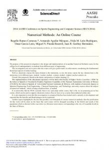
2. Methods of Investigation and Mean-Flow Characteristics 2.1. Experiment The experiments were carried out in the low-turbulence wind tunnel T-324 of the ITAM which has a test section of 1 m × 1 m and 4 m length. Background disturbances in the free stream were less than 0.02% in a frequency range higher than 1 Hz. A sketch of the experiment is shown in Figure 1 together with the coordinate system used. A flat plate having a chord length of 1.5 m, a span of 1 m, and a thickness of 10 mm was installed in the test section at a zero angle of attack. The leading edge was composed of two conjugated semi-ellipses (see Kachanov et al. (1975) for more detail). A hot-wire anemometer with a linearizer was used for the velocity measurements. The probe consisted of a single Wollaston-type wire (platinum covered with copper) with a sensitive element of 0.3 mm length and 6 µm diameter providing a spanwise resolution of about 0.15 mm. It was mounted on a traverse which allowed us to set its streamwise (x), spanwise (z), and normal-to-wall (y) positions with high accuracy. The experiments were carried out at controlled disturbance conditions with an ‘artificial’ excitation of a primary instability wave by means of an experimental technique similar to that used by Borodulin and Kachanov (1995). A vibrating ribbon was placed 250 mm from the plate leading edge over a spanwiseoriented strip of adhesive tape pasted onto the plate. When an electric current (produced by a signal generator) passed through the ribbon, it oscillated in a magnetic field generated by a permanent magnet positioned under the plate. The strip had a gap (with a width of about 2 mm) at approximately z = 0. The ribbon was excited at a frequency of 81.4 Hz and produced an initial perturbation which starts as an almost two-dimensional disturbance with a tiny local distortion in the spanwise distribution of the mean-flow velocity and the disturbance amplitude at z = 0. The non-uniformity fixed the single ‘peak’ position and provoked the subsequent formation of Λ-vortices and other transitional structures discussed in the present paper. The single peak position has been chosen for the present experiments (and DNS) in order to avoid possible interactions between adjacent structures in the spanwise direction. In the absence of initial perturbations (i.e. when the vibrating ribbon was not actuated) the mean flow in the boundary-layer corresponded to the Blasius flow with very high accuracy. In all present measurements the free-stream speed was constant: U0 = 9.18 m/s. In the chosen regime of excitation the streamwise components of the mean velocity field U(x, y, z) and the instantaneous disturbance field u � (x, y, z, t) were documented in the range x = 430 to 550 mm (Reynolds numbers Rex = U0 x/ν =
Figure 1. Sketch of experiment. 1 – wind tunnel test-section walls; 2 – flat plate; 3 – traversing mechanism; 4 – hot-wire probe; 5 – vibrating ribbon; 6 – permanent magnet; 7 – strip of adhesive tape; all units in millimeters.
321
Late-Stage Transitional Boundary-Layer Structures. Direct Numerical Simulation and Experiment
2.69 × 10⁵ to 3.44 × 10⁵), y = 0 to 9 mm, and z = −15 to 13 mm. In the streamwise direction this domain starts with the formation of the Λ-structures and ends at the almost turbulent (near-wall) flow. The most detailed measurements presented in this paper were performed at x = 450 and 500 mm where the instantaneous velocity fields were documented in the (y, z)-planes as sets of y-profiles with a spanwise step of ∆z = 1 mm close to the peak position (from z = −2 to +2 mm at x = 450 mm and from z = −4 to +4 mm at x = 500 mm) and with a step of 2 mm farther away from the peak position. The step in the y-direction was variable (between 0.1 mm very near the wall and 0.5 mm outside the boundary-layer edge). Data acquisition of the hot-wire signals was performed on a computer after passing the signals through a low-frequency filter (with a cut-off frequency of 2 kHz) and sampling with 59 points per fundamental period (i.e. with a sampling frequency of 4800 Hz). The data recording was synchronized with the generator that fed the vibrating ribbon. The main experimental results presented in this paper were obtained after ensemble averaging of the hot-wire signals for 200 fundamental periods of the disturbance during approximately 10 s. This procedure was necessary to reduce the non-periodic part of perturbations and to obtain the phase-locked, ensemble-averaged instantaneous three-dimensional disturbance fields for the periodic part. The non-periodic perturbations, caused by the beginning flow randomization observed at the late stages of transition, were documented as well. 2.2. Direct Numerical Simulation The numerical method used here has already been described in Fasel et al. (1990), Kloker et al. (1993), and Rist and Fasel (1995), for instance. It is based on the vorticity-velocity formulation of the Navier–Stokes equations for incompressible fluids. The flow is split into a two-dimensional steady base flow, which in the present case corresponds to the Blasius boundary-layer, and an unsteady three-dimensional disturbance flow. The non-linear modification of the base flow by large-amplitude disturbances is represented by the (temporal) mean of the disturbances. For discretization, the governing equations are first transformed into Fourier space and the transformed equations are discretized by standard fourth-order-accurate central finite differences in streamwise and wall-normal directions as described in Rist and Fasel (1995), except for the x-convection terms which are discretized by one-sided finite differences which exhibit fourth-order accuracy when applied in an alternating up- and downwind manner. The initial conditions for the simulations are zero disturbances throughout the integration domain. Disturbances are introduced through a suction and blowing slot at the wall as described below. At the inflow boundary, which is placed one Tollmien–Schlichting (TS) wavelength upstream of the disturbance strip, zero disturbances are assumed for all time, at the free-stream boundary the vorticity is zero and the velocity decays exponentially for y → ∞. The “relaminarization zone” by Kloker et al. (1993) which reduces the disturbance vorticity to zero is applied starting two TS wavelengths upstream of the end of the integration domain. The vorticity at the wall is computed from the conditions specified in Kloker et al. (1993) and Rist and Fasel (1995) which take into account the zero divergence of the velocity and the vorticity vectors. Based on the solution of the previous time step the non-linear convection terms in the discretized vorticity-transport equations (one for every component of the three-dimensional vorticity vector) are computed using the pseudo-spectral technique introduced by Orszag (1971). Time integration is then performed applying the standard fourth-order-accurate four-step Runge–Kutta scheme. The instantaneous wall-normal velocity component at the wall within the disturbance strip is prescribed by νw (x, z, t) = νa (x) · ATS · sin(β · t) + A3D · νs (x) · g(z)
x1 ≤ x ≤ x2 ,
for
(1)
where x 1 and x 2 are the beginning and end of the disturbance strip, respectively. Thus, a two-dimensional TS wave with frequency β and a steady three-dimensional disturbance may be forced by specifying the amplitude ATS and A3D , respectively. Here, the ν distribution versus x is defined by the polynomials � 81 � 5 3ξ + 8ξ 4 + 6ξ 3 − ξ 16 � 81 � 5 νa (ξ) = 3ξ − 8ξ 4 + 6ξ 3 − ξ 16 νa (ξ) =
and νs (ξ) = −3ξ 4 − 8ξ 3 − 6ξ 2 + 1 for
ξ λz0 , 0 2 4 which simulates a single roughness element at z = 0 that produces a streamwise row of Λ-vortices in connection with the harmonic two-dimensional forcing with ATS . The function g(z) fulfills � ∞ the conditions that the forcing around z = 0 remains unaltered with respect to the periodical case and −∞ g(z) dz = 0. Using this function (and the same frequency as in the periodical case) the influence of the spanwise periodicity on K -type transition was investigated in Meyer et al. (1998) by increasing the spanwise distance of adjacent ‘peak’ planes compared with the simulations of Rist and Fasel (1995) which have used g(z) = cos(γ0 z) for all z. For the present comparisons the case with λz = 3λz0 , i.e. γ0 = 3γ , has been selected. The integration domain starts at Reδ1 = 580 with a height of 12δ1, where δ1 is the boundary-layer displacement thickness, the spanwise period is λz = 73.5 mm, and the disturbance strip extends from Reδ1 (x 1 ) = 637 to Reδ1 (x 2 ) = 684. A discretization with 1050 grid points in x and 129 grid points in y has been used together with 209 conjugate complex de-aliased Fourier modes. Using equidistant grid spacing in all directions, the step sizes correspond to ∆x = 0.384 mm, ∆y = 0.0897 mm, and ∆z = 0.3535 mm. Time is discretized with 300 time steps per disturbance period (frequency f = 98.4 Hz, free-stream velocity U0 = 9.18 m/s) and the disturbance amplitudes in (1) are ATS = 0.5 × 10⁻² and A3D = 0.13 × 10⁻³. 2.3. Frequency Influence on the Present Results Actually the present work compares two realizations of the same transition scenario with somewhat different frequencies ( f = 81.4 Hz in the experiment and f = 98.4 Hz in the DNS). Firstly, because of our decision to compare results from an earlier simulation series with experiments performed independently. Secondly, because such a comparison allows us to assess the frequency influence (or independence with respect to the observed structures) of the results at hand. This second aspect is further corroborated by additional experiments which have been performed with a modified disturbance input that produced non-periodical isolated (i.e. single) beatings of approximately the same amplitude as in the periodical case discussed so far (see Borodulin et al., 2000). In frequency space this set-up is characterized by a continuous spectrum in contrast to the discrete frequencies of harmonic forcing. Especially, there is no distinct frequency, which could influence the results. All other parameters of the set-up described in Section 2.1 remained unchanged. In these experiments exactly the same structures developed further downstream of the disturbance source. However, there was only one structure in each realization without any periodicity at all. Close qualitative agreement of the late-state structures with those found in the periodical case is illustrated in Figure 2 obtained by Borodulin et al. (2000) for the 4-spike stage. The top plot corresponds to the periodical case, while the bottom plot is obtained for pulse-like excitation. In this pulse case the Λ-structures, the ring-like vortices, and all associated phenomena are practically the same (within experimental accuracy) as those found at the fixed frequency of the primary instability wave. The most visible differences observed in the pulse case are associated with the presence of: (i) a low-speed region positioned under the first ringlike vortex and (ii) an elongated high-speed region positioned behind the main structures near the wall. As was shown by Borodulin et al. (2000), these phenomena are explained in the following way. In the localized wave packet of the excited TS waves it was impossible to avoid weak fluctuations associated with the previous and subsequent periods of perturbation. These fluctuations had much lower amplitudes but they were amplified downstream and were visible at all stages of the disturbance development. The speed of the Λ-structure and, especially, the ring-like vortices increased quickly downstream and became significantly larger than the phase speed of previous and subsequent periods of the wave packet. As a result, the structure reaches the previous period (the white spot under the first ring-like vortex) and crawls over it. Simultaneously, the structure runs away from the subsequent period leaving behind itself a long region with a relatively high speed.
Late-Stage Transitional Boundary-Layer Structures. Direct Numerical Simulation and Experiment
323
Figure 2. Comparison of streamwise disturbance velocity u � /U0 in the (y, t)-plane at z = 0 in Borodulin et al. (2000). Top – experiment with periodic forcing; bottom – experiment with one-time pulse-like forcing.
The similarity of the structures illustrated by Figure 2, as well as all subsequent plots presented in this article, indicate that the only significant difference, observed when the excitation frequency changes, is the distance between succeeding breakdown stations (and the associated spike- and Ω-structures), which increases with decreasing frequency. The local dynamics of structures is frequency independent! Thus, the present results show that our observations are not due to particular parameters of the experiment or the simulation, nor to the choice of a certain frequency. These structures appear in a very wide range of variations of the initial disturbance spectra; including turbulent flows where the initial spectra are completely different from the two cases studied here and, in particular, the weakly non-linear stages of development might be bypassed completely. Some additional confirmation of this point can also be found in Bake et al. (2000) and Kachanov (2000).
3. Formation of �-Structures and Spikes The results presented in this section were obtained at a relatively early stage of the disturbance development which is usually called the “1-spike stage” and corresponds to the streamwise coordinate x = 450 mm in the present experiment (i.e. Reynolds number Rex = U0 x/ν = 2.82 × 10⁵) and x = 430 mm in the DNS (Rex = 2.61 × 10⁵). The difference in the streamwise coordinates is caused by a difference in the initial disturbance spectra in the experiment and DNS (as already discussed in Section 2.2). There are three main goals for presenting the results obtained at the 1-spike stage: (i) to show that the same structures are observed both in DNS and in experiment, (ii) to demonstrate that these structures are characteristic for the 1-spike stage of boundary-layer breakdown despite the different initial disturbance spectra used for both cases, and (iii) to demonstrate the structures’ properties in somewhat more detail than in previous studies. The results presented in this section are very useful for understanding the subsequent discussion of later stages of the transitional flow presented in Section 4. 3.1. Three-Dimensional High-Shear Layer and First Spike The earliest and most typical indication for the development of coherent structures in the non-linear region of laminar-turbulent transition in a boundary-layer consists of the formation of a three-dimensional HS layer. Contour plots of the intensity of the spanwise component ωz of the vorticity disturbance vector (i.e. without mean vorticity) in the (y, t)-plane are shown in Figure 3 for comparison of the shape of
324
V.I. Borodulin et al.
Figure 3. High-shear layer at the 1-spike-stage in the (y, t)-plane. Contours of spanwise component ωz of the vorticity disturbance vector. Left – experiment ((a),(b) peak position and 2 mm off peak); right – DNS ((a),(b) peak position and 2.12 mm off peak). White squares in (a) indicate the spike positions. Fifteen contour levels: −0.238 − 0.248/0.0347; dark shades of gray correspond to high values.
the HS layer obtained in the present experiments and DNS for the 1-spike stage at two different spanwise positions. For the experimental data ωz ≈ ∂u/∂y is used to approximate the spanwise component of vorticity. As for other figures, which follow, the time axes are plotted to the same scale in order to show the frequency influence discussed in Section 2.3. The flow field in the experiment is, of course, not as periodic and symmetric with respect to z as in the DNS due to background disturbances in the wind tunnel. However, besides minor differences, all relevant flow structures appear in both realizations. Indeed, the local agreement of the HS layer is of a quantitative nature (same iso-levels in experiments and simulation) and the lower frequency leads to a greater distance between the structures, as already expected from Figure 2. The same agreement has been found for other spanwise sections of the structure (not shown). A displacement away from the peak position in Figure 3(b) reveals the following properties of the structures: (i) a time delay of the HS layer as a whole, (ii) a decrease of its intensity, (iii) a reduction of the HS layer’s (temporal) length, (iv) the appearance of another HS layer located closer and more parallel to the wall, and (v) the formation of very stretched elongated streaks with rather high as well as low shear intensity at the largest distance from the peak position (not shown in Figure 3). In addition, the positions of the |u � | spike maxima are indicated by white squares for reference. The spike appears immediately under the kink close to the top of the HS layer. The spanwise location of the spikes and their wall-normal position with respect to the Λ-structures can be observed in Figure 4 where iso-lines of the u-component of the velocity disturbance are presented in the (z, t)-plane for two distances from the wall. Dark spots at the largest distance (Figure 4(a)) indicate regions of very large magnitudes of the negative instantaneous velocity disturbance and correspond to the spikes. Closer to the wall these spots deform into Λ-shaped structures with a rather low flow velocity in their ‘legs’ (Figure 4(b)). Apart from some asymmetry with respect to z = 0 the presentation of the experimental data is biased by the coarser step size in z compared with the DNS. In addition, the experiment shows the phase average of several individual events whose spatio-temporal positions can vary and thus smear the picture while the DNS displays an instantaneous picture. This explains the differences close to the peak position (i.e. around z = 0) where the DNS shows rather tiny structures with large spanwise gradients. However, the distance between the structures with respect to their duration increases for the lower frequency and Figure 4 also demonstrates a reasonable agreement between calculated and measured data.
Late-Stage Transitional Boundary-Layer Structures. Direct Numerical Simulation and Experiment
325
Figure 4. Relationship between spike and Λ-structure at the 1-spike-stage. Contours of streamwise velocity disturbance u in the (z, t)-plane. Left – experiment ((a),(b) 3 and 1.4 mm from the wall); right – DNS ((a),(b) 2.87 and 1.32 mm from the wall). Ten contour levels: −0.1 − 0.1/0.0222; light shades of gray correspond to high values.
3.2. “Multi-face” Structure of the � The term ‘Λ-structure’ has been very widely used by researchers for many years and is probably borrowed from the term ‘Λ-vortex’ introduced by Hama and Nutant (1963) based on flow visualizations. In many studies the terms ‘Λ-structure’ and ‘Λ-vortex’ were used, however, in a qualitative manner for description of some flow patterns obtained at non-linear stages of transition either in experiments or DNS. In this section we try to outline in more detail what the terms ‘Λ-structure’ and ‘Λ-vortex’ mean from a quantitative viewpoint, as well as to show the relationship between different Λ-patterns observed in the boundary-layer. The Λ-structure is inclined to the wall at a certain angle and its different parts appear at different distances from the wall (see Figures 3 and 4). Therefore, in order to show the shape of the structure as a whole it is convenient to use projections of the experimental and DNS data onto the (z, t)-plane. In the present study several projections of different instantaneous quantities were investigated and analyzed, namely for: (i) the total streamwise velocity field, (ii) the velocity disturbance field, (iii) the total spanwise vorticity field, and (iv) the spanwise disturbance vorticity field. One of these projections, namely the projection of the instantaneous spanwise vorticity disturbance (iv) 1 ωzΣ = L
7� mm
ωz (y)∆y ,
(4)
y=1 mm
where L = 6 mm, is presented in Figure 5. It depicts a Λ-shaped HS layer similar to that observed by Kovasznay et al. (1962) which they called “∆-wing shaped.” Very similar structures have been found for the three other projections ((i)–(iii)) listed above. It turned out that a Λ-shaped structure appears in all variables studied for the 1-spike stage centered around the peak plane at z = 0. Figure 6 depicts visualizations of the Λ-vortex itself, either as hydrogen bubbles in water (Figure 6(a)) or calculated and visualized with the help of the so-called λ2 -method (Figure 6(b)) for approximately the same stage of the disturbance development. This method (see Jeong and Hussain, 1995) identifies flow regions with negative pressure disturbance bound by inflection points of the pressure gradient in a plane perpendicular to the vortex axis. In this way it is able to distinguish between regions of rotating fluid while ignoring
326
V.I. Borodulin et al.
Figure 5. Λ-structure at the 1-spike-stage in the (z, t)-plane as contours of spanwise component ωz of the vorticity disturbance vector obtained by integration in the wall-normal direction. Left – experiment; right – DNS (dotted lines marked 1–3 correspond to the time instants used in Figures 6 and 7). Ten contour levels: −0.6 − 0.9/0.1667; dark shades of gray correspond to high values.
Figure 6. Visualizations of a Λ-vortex in (x, y, z)-space. (a) Hydrogen bubbles in a water-channel experiment, (b) iso-surface of a λ2 -eigenvalue (Jeong and Hussain, 1995) which encloses regions of rotating fluid from DNS (the 1-spike-stage corresponds to x = 430 mm.).
areas with high vorticity but without rotation of the fluid, as has been verified by Rist et al. (1998). In Figure 6 the elongated legs of the Λ-vortex are clearly visible, as well as the erecting ring-like vortex structure at its downstream tip (the Ω-vortex). The strong negative velocity disturbance referred to as spike is located in the center of the Ω-vortex where it is generated by induction through the motion of the vortex. Regardless of which criterion is used (as in Figures 4–6) the most significant structures that appear in the flow at the 1-spike stage of the transition development have a Λ-shape both in DNS and in experiment. This fact is probably explained by a predominating role of the Λ-vortex in the instantaneous flow field (Figure 6). An intensive rotation of the fluid in the Λ-vortex legs leads to a displacement of the low-speed fluid away from the wall between the two legs, as well as to a displacement of the high-speed fluid toward the wall, thus outlining the vortex. For this reason, the regions of low-speed fluid, high-speed fluid, and the HS layer (po-
Late-Stage Transitional Boundary-Layer Structures. Direct Numerical Simulation and Experiment
327
sitioned near the upper border of the low-speed region) exhibit a Λ-shape as well (see Figures 4 and 5). It seems reasonable to use the term ‘Λ-structure’ for each of the flow patterns as those shown in Figures 4–6 (or for all Λ-shaped patterns together) as a general notion characterizing the disturbance structure. Meanwhile, the term ‘Λ-vortex’ has a more strict sense designating the real rotating vortex (Figure 6) with a low-pressure region inside of it caused by centrifugal forces. 3.3. Wall-Normal Structure of Perturbations The rather complicated shape of the Λ-structure in the wall-normal direction is illustrated in Figures 7 and 8. In Figure 7 the measured and calculated iso-lines of the absolute value of the gradient of the total streamwise velocity is shown in the (y, z)-plane at two time instants (indicated in Figure 5 as lines 1 and 3). The gradient is defined here as
�
� ∂(U + u) 2 ∂(U + u) 2 |grad{u(y, z)}| = + . (5) ∂y ∂z At the 1-spike stage this gradient is very closely related to the spanwise component Ωz + ωz of the total vorticity vector because the spanwise derivatives in (5) are much smaller than the wall-normal derivatives. (Also note that the derivatives ∂(V + ν)/∂x are much smaller than ∂(U + u)/∂y in the whole region of measurements and calculations.) The close agreement of (5) with the spanwise vorticity component has been confirmed by comparing the instantaneous fields of the total spanwise vorticity measured and calculated for
Figure 7. Two wall-normal sections of a Λ-structure at the 1-spike-stage. Contours of the total streamwise velocity gradient in the (y, z)-plane: time instants (a) 1 and (b) 3 shown in Figure 4. Left – experiment; right – DNS. Fifteen contour levels: 0.0 − 1.0/0.0714; dark shades of gray correspond to high values.
Figure 8. Relative positions of the Λ-vortex and the HS layers. Contours of the total streamwise velocity gradient in the (y, z)-plane together with velocity vector field (ν, w) obtained at the 1-spike-stage in DNS at time instant 2 shown in Figure 4. Fifteen contour levels: 0.0 − 1.0/0.0714; dark shades of gray correspond to high values.
328
V.I. Borodulin et al.
the same stage of transition (not shown here). The use of the velocity gradient |grad{u(y, z)}| is very convenient for comparison with subsequent stages of the transition development discussed below in Section 4. Figure 7 shows that, similar to the Λ-vortex (Figure 6), the three-dimensional HS layer is inclined to the wall. When time increases it splits into two ‘legs’ which move away from the peak position and approach the wall, similar to the Λ-vortex legs (see Figure 6). In addition to Figure 7, one of the DNS-data plots (for time instant 2 shown in Figure 5) is presented in Figure 8 together with the instantaneous velocity vectors in the (y, z)-plane in order to show the relationship between the Λ-vortex and the HS layers. It is seen from these figures that the Λ-structure has several layers in vertical direction with an alternating low and high streamwise velocity gradient (and hence spanwise vorticity). The velocity vectors indicate counter-rotating vortices connected with the legs of the Λ-vortex. This rotation leads to the formation of the main (most intensive) HS layer at a relatively large distance from the wall all along the Λ-structure, i.e. above its tip and its legs. The HS layer appears due to the displacement of the low-speed fluid away from the wall. In the near-wall region (and at the side of the peak position in the z-direction) two other HS layers are observed which are caused by a displacement of the high-speed fluid toward the wall due to the rotation in the legs of the Λ-vortex. Between these two HS layers two regions with relatively low shear are observed both in DNS and experiments. Note that these regions of low shear coincide with the centers of the legs of the Λ-vortex, i.e. almost no streamwise velocity gradients are observed in the vortex cores.
4. Subsequent Development of Structures and Their Role in Flow Randomization The subsequent development of the structures discussed above, as well as their role in the process of flow randomization, was investigated in detail. Some results of this study are presented in this section. The most detailed comparison of the experimental and numerical data is performed for the so-called “3-spike stage” of the transition process which corresponds to the streamwise coordinate x = 500 mm in the experiment (Rex = U0 x/ν = 3.13 × 10⁵) and x = 455 mm in the DNS (Rex = 2.76 × 10⁵). The spatial structure of the perturbations at this stage is investigated in Sections 4.1 and 4.2, while Section 4.3 is devoted to a study of the interaction of the structures with the near-wall region, as well as to their role in the beginning of the flow randomization. 4.1. �-structures at the 3-Spike Stage The Λ-structures are still present in the flow at the 3-spike stage. This fact is illustrated in Figure 9(a) by contour lines of the streamwise velocity disturbance projected onto the (z, t)-plane as uΣ =
1 L
7� mm
u(y)∆y ,
(6)
y=1 mm
where L = 6 mm. A weak initial asymmetry of the structures observed in the experiment is more pronounced at this late stage. As far as the coarser spanwise resolution in the experiment allows us to observe, the general shape and scale of the Λ-structures remain the same in the numerical and experimental pictures. Similar patterns have been observed for projections of other flow variables, too (not shown). In addition to the Λ-structure two localized perturbations occurring ahead of its tip can be observed in Figure 9(a). The streamwise velocity disturbance has very large negative values in the centers of these localized structures and positive values at their sides. These structures correspond to the first and the second spikes in time-traces. The third spike is also present in both experimental and DNS time-traces but it is still coupled with the Λ-vortex tip and hence no longer discernible in the experimental projection plot in Figure 9(a). (This is an example of the benefits of performing close comparisons between experiments and DNS, as presented here.) At the same time, the low-speed regions (associated with spikes) are very well seen at larger distances from the wall. Their spatial shapes in the (z, t)-plane can be inferred from Figure 9(b) from contours of the u-component of the velocity disturbance. Because of different wall distances compared with the spikes the Λ-structure is no longer visible in Figure 9(b) in the experiment and weakly developed in the
Late-Stage Transitional Boundary-Layer Structures. Direct Numerical Simulation and Experiment
329
Figure 9. Λ-structures and localized low-speed regions associated with spikes in the (z, t)-plane at 3-spike-stage. Contours of streamwise velocity disturbance u. (a) Result of integration in the wall-normal direction; left – experiment: 10 contour levels: −1.8 − 1.3/0.3444, right – DNS: 10 contour levels: −5.0 − 2.5/0.8333. (b) Streamwise velocity disturbance u at fixed distance to the wall; left – experiment, y = 4.2 mm, 15 contour levels: −0.063 − 0.015/0.0056, right – DNS, y = 3.0 mm, 15 contour levels: −0.13 − 0.07/0.0143. Light shades of gray correspond to high values.
simulation. The first spike appears at the largest distance from the wall, the second one closer, and the third even closer to the wall (see also Figure 12 below). The time interval between the spikes is practically the same in simulation and experiment while the distance between the two groups of spikes increases due to the lower frequency in the experiment. Every low-speed region is surrounded by rather weak high-speed regions. The shapes of these localized structures and their spatial positions are very similar in Figure 9(b) in simulation and experiment. It is important to note that, in contrast to the experiments by Knapp and Roache (1968), absolutely no evidence of a flow breakdown was observed in the vicinity of the Λ-vortex legs even at the 3-spike stage, neither in the experiments nor in the DNS. Instead, the shape of the legs evolves gradually downstream and changes only slightly without any significant small-scale distortions. 4.2. Spikes and Ring-Like Vortices The shape of the localized structures observed at the 3-spike stage which has been studied in more detail is discussed now. Figure 10(a) shows contour plots of the u-velocity disturbance in the (y, z)-plane for the time instant which corresponds to the first spike. The position of the spike maximum is indicated with a square. It can be seen that the region of low-speed fluid (which corresponds to the spike) has a shape close to a circle and the instantaneous velocity disturbance has its lowest values inside this region (at the time moment shown). A weak positive velocity disturbance surrounds the spike region at the very moment when it appears. Such a simultaneous fluctuation of the streamwise velocity component in the negative direction inside the spike region and in the positive direction around it (see also Figure 9) indicates the presence of a ring-like vortex around the spike region shown in Figure 10(a). The ring-like structure of the disturbances attributed to the spike at late stages of the transition development was already suggested from previous experiments (Borodulin and Kachanov, 1995) based on observations in the peak plane only. It was also supported by pictures obtained from DNS by Rist and Fasel
330
V.I. Borodulin et al.
Figure 10. Shapes of localized low-speed regions (a) and ring-like structure of disturbances (b) associated with spikes in the (y, z)plane at the 3-spike-stage for a time instant that corresponds to the first spike. (a) Contours of streamwise velocity disturbance u; left – experiment, 15 contour levels: −0.374 − 0.108/0.0344; right – DNS, 15 contour levels: −0.315 − 0.168/0.0345; light shades of gray correspond to high values. (b) Contours of the total streamwise velocity gradient; left – experiment, right – DNS; 15 contour levels: 0.13 − 1.3/0.0834; dark shades of gray correspond to high values. Squares indicate position of first spike.
(1995) and Rist and Kachanov (1995). In the present paper we perform a direct comparison of the spatial structure of the ring-like vortex obtained in DNS and experiment. A ring-like vortex centered around the peak position (z = 0) is displayed in Figure 10(b) for the time instant corresponding to the first spike by means of contour plots of the gradient of the total streamwise velocity (5) in the (y, z)-plane. The position of the spike maximum is again marked with a square. These pictures obtained at the 3-spike stage can be compared with those presented above for the 1-spike stage. The most significant difference is that at the 1-spike stage (Figures 3 and 4) the first spike is positioned under a kink of the HS layer near the Λ-vortex tip, while at the 3-spike stage (Figure 10(b)) it is observed in the center of the ring-like vortex which is separated from the Λ-structure. At the same time, the first spike occurs much farther away from the wall, near the external edge of the boundary-layer. The shapes of the rings are very similar in DNS and experiment, as well as their placement in the outer part of the boundary-layer. This agreement is observed despite the difference in the initial disturbance conditions in simulation and experiment and suggests the universality of these boundary-layer structures, as well as the processes connected to their development. The most significant difference between the experimental and theoretical pictures presented in Figure 10(b) is the (dimensional) y-position of the ring-like vortices together with somewhat more intensive streamwise vortices in the numerically simulated regime compared with that studied in the experiment. The reason for the latter is a higher spatial resolution and the absence of any averaging due to random fluctuations in the presentation of the simulation data, while larger x-stations and the possibility of a very small streamwise adverse pressure gradient could be responsible for the larger boundary-layer thickness in the experiments. 4.3. Perturbations Induced in the Near-Wall Region One of the most important open questions in understanding the physical nature of late non-linear stages of boundary-layer transition is connected with the mechanisms of flow randomization, i.e. the ways of rapid amplification of some background (non-deterministic) perturbations that cause the flow to become stochastic. From the observations in Figures 9 and 10 one might speculate that the ring-like vortices associated with the spikes influence the flow field closer to the wall. Indeed, the flow randomization in the present experiments started in the vicinity of the peak position in the near-wall region. This fact is illustrated by three pairs of time-traces presented in Figure 11(a)–(c) measured at y = 4.5, 1.7, and 0.2 mm, respectively, at x = 505 mm and z = 0. Here, the direct read-outs of the hot-wire anemometer are drawn as lines and compared with their ensemble average shown as circles. Thus, the non-periodicity of the velocity fluctuations at this stage becomes clearly visible. Far away from the wall (Figure 11(a), y = 4.5 mm) the spikes in the actual instantaneous time-trace (lines) exhibit some variations of their magnitude and temporal position from one fundamental period to another. This process is more pronounced for the second and third spikes than for the first. A similar non-periodicity is observed closer to the wall for the time-traces at y = 1.7 mm (Figure 11(b)).
Late-Stage Transitional Boundary-Layer Structures. Direct Numerical Simulation and Experiment
331
Figure 11. Beginning of flow randomization at the 3-spike-stage. Time-traces of streamwise velocity disturbance u obtained in experiment in the peak position: y = 4.5 (a), 1.7 (b), 0.2 (c), and 0.2 mm (d). 1 – not averaged; 2 – ensemble-averaged. In (d) 20 unaveraged time-traces from different fundamental periods are superimposed.
Very close to the wall (Figure 11(c), y = 0.2 mm) this non-periodicity is much stronger than the periodic perturbation. Because of their characteristic appearance on an oscilloscope screen the stochastic beatings of the near-wall traces have been called ‘fire.’ As shown in Figure 11(d) the ‘fire’ involves a set of positive velocity peaks whose magnitude and position (within the fundamental period) change from one fundamental period to the next. The random fluctuations associated with the ‘fire’ exhibit exponential growth in the downstream direction: at y = 0.28 mm from the wall their amplitude for the 1-, 2-, and 3-spike stages are 2%, 4%, and 12%, respectively, when compared with the local (mean) velocity and 0.3%, 0.7%, and 2.5% with respect to the free-stream velocity. The disturbance field associated with the fire-like signals is presented in the (y, t)-plane in Figure 12(a) for the experimental and DNS data obtained at the 3-spike stage in the vicinity of the peak position. Some positive small-scale velocity fluctuations are observed in the regions marked with dashed lines. The characteristic time scale of each of these fluctuations is about 5% of the fundamental period. Comparison of Figure 12(a) and (b) (obtained in the peak position) clearly shows that every positive velocity fluctuation
332
V.I. Borodulin et al.
Figure 12. Near-wall perturbations induced by ring-like vortices at the 3-spike-stage. Contours of streamwise velocity disturbance u in the (y, t)-plane: (a) off peak (2 mm in experiment, 1.77 mm in DNS), (b) peak position. Left – experiment; right – DNS. Positive small-scale velocity fluctuations are marked with a dashed line, while the corresponding negative velocity fluctuations (associated with ring-like vortices) are marked with a dotted line. Fifteen contour levels: −0.25 − 0.15/0.0286; light shades of gray correspond to high values.
(a “positive spike”) seen in Figure 12(a) corresponds to a strong negative velocity fluctuation (a usual spike) seen in Figure 12(b). (The corresponding regions are marked with dotted lines in the latter case.) Thus, the spikes in the time traces of Figure 11(a), which are a manifestation of the first, second, and third (incipient) ring-like vortex (see Sections 4.1 and 4.2, Figures 9 and 10), appear to cause the positive fluctuations in the near-wall region in a similar way to those observed in the spanwise direction in Figure 9 or all around the vortex as in Figure 10(b). The spikes and the associated ring-like vortices propagate in the outer part of the boundary-layer, while the positive spikes (the “fire tongues” in Figure 11(d)) appear quite close to the wall. The experimental and DNS results demonstrate good agreement of the development of the relevant structures and thus confirm each other. One fundamental difference between the experimental and numerical data compared here is that the numerical data are instantaneous while the experimental data consist of a periodic component (the ensemble average) and a significant non-periodic (irregular) component which is particularly large in the near-wall region (see curves 1 in Figure 11(b)–(d)). This non-periodic part is hard to determine from DNS because an averaging over many periods as in experiments would be necessary, which is very expensive. Another reason for using instantaneous data in the simulations is the fact that it is not practicable to try to reproduce the background perturbations of an experiment in a simulation. These perturbations are strongly amplified at the late stages of transition and are thus very sensitive to their initial amplitudes. The results would probably be hard to compare. Nevertheless, we know from measurements that non-periodicity is tightly connected with the positive spikes (the “fire tongues”) marked in Figure 12(a) and just represents fluctuations of the spatiotemporal position of the positive fluctuations from one fundamental period to the next (Figure 11(b), (c)). During the ensemble averaging of the experimental time-traces these fluctuations lead to a reduction of the periodic-disturbance magnitudes and to a more dispersed distribution of the averaged perturbations in time and space. In particular, the averaging in the experiment lets the ring-like vortices (and spikes) appear larger in time and in space and the positive spikes, associated with the “fire tongues,” penetrate to the exact peak position (Figure 12(b) left underneath the spikes) in contrast to the DNS (Figure 12(b) right) where the flow is instantaneous. The strong spanwise gradient of the instantaneous velocity is most clearly visible in the DNS data in Figure 10(a) (right) in the vicinity of the peak position under the ring-like vortices (between y = 0 and at y ≈ 2 mm). When the spikes exhibit small variations of their spatio-temporal position from one fundamental period to another this gradient produces very strong non-periodic fluctuations in the near-wall
Late-Stage Transitional Boundary-Layer Structures. Direct Numerical Simulation and Experiment
333
Figure 13. Contours of instantaneous velocity disturbance u in the (x, y)-plane: (a),(b) time instant t = 0.85 T; (c),(d) time instant t = 0.9 T; (a),(c) peak position; (b),(d) 1.77 mm off peak. DNS results. Negative (normal) spikes are marked with white squares while positive spikes are marked with black squares. Fifteen contour levels: (a),(c) −0.25 − 0.15/0.0286; (b),(d) −0.23 − 0.22/0.0321; light shades of gray correspond to high values.
region. This circumstance explains why the strongest irregular motions are observed experimentally in the peak position under the ring-like vortices. The experiment shows that the near-wall positive spikes are phase coupled with the spikes (i.e. with the ring-like vortices) propagating in the outer part of the boundary-layer. The downstream speed of the two types of fluctuations is found to be exactly the same and close to the free-stream velocity despite the fact that the positive spikes appear rather close to the wall where the local mean-flow velocity is about 0.65 (at y = 1.6 mm). The DNS results also show that the structures attributed to the positive spikes are phase coupled with the ring-like vortices, i.e. with the spikes. This fact is illustrated in Figure 13 where the instantaneous velocity field in the (x, y)-plane is shown for two consecutive time instants, t = 0.85 T (Figure 13(a),(b)) and t = 0.9 T (Figure 13(c),(d)), at z = 0 (Figure 13(a),(c)) and z = 1.77 mm (Figure 13(b),(d)), respectively. The speed of the positive spikes (connected with the “fire tongues”) is significantly higher than the local velocity of the surrounding flow but it is practically equal to the speed of the ring-like vortices, i.e. c/U0 ≈ 0.78 and 0.56 for the first and second spikes, respectively. Taking into account that the ring-like vortices contain much disturbance energy and dominate in the high-frequency and small-scale range of the disturbance spectrum, the unusually high speed of the near-wall positive spikes (higher than the local velocity), phase coupled with the ring-like vortices, clearly indicates that the near-wall perturbations are induced by the ring-like vortices. The important role of the near-wall perturbations induced by the ring-like vortices is illustrated in Figure 14 where the instantaneous spanwise vorticity fields (measured and calculated) are presented in the
334
V.I. Borodulin et al.
Figure 14. Vorticity induced by ring-like vortices in the near-wall region at the 3-spike-stage. Contours of spanwise component ωz of the vorticity disturbance vector in the (y, t)-plane. Left – experiment ((a) 2 mm off peak, (b) peak position), right – DNS ((a) 1.77 mm off peak, (b) peak position). Fifteen contour levels: −0.32 − 0.49/0.0579; dark shades of gray correspond to high values.
(y, t)-plane at the 3-spike stage for two spanwise positions. In general, the experimental and DNS pictures again look very similar. However, due to the presence of irregular motions and their averaging, discussed above, the DNS results show the near-wall vortical structures attributed to the positive velocity spikes clearer (Figure 14(a) right, y ≈ 1 mm). At the off-peak position (where the ring-like vortices are absent and the HS layer is weak) the induced vorticity dominates in the y-region between approximately 0.6 and 1.6 mm and represents undoubtedly the strongest high-frequency (small-scale) perturbation for the whole range of the ycoordinate. Note also that the induced near-wall perturbations form a new HS layer observed in Figure 14(a) at y ≈ 1 mm. Comparison of the experimental and numerical results at the peak station in Figure 14(b) clearly shows where and when the most intensive irregular motions appear. From the spectral point of view the irregular component of the near-wall fluctuations, induced by the ring-like vortices, consists mainly of low-frequency perturbations below the fundamental frequency. The results of Dryganets et al. (1990) indicate that these perturbations can be amplified by means of a subharmonic-type resonant interaction during the next stage of laminar-turbulent transition, and perhaps in turbulent flows, as well. However, this needs further investigation in the future.
5. Discussion and Conclusions The mechanism responsible for the initial stages of formation of the ring-like vortices is one of the most important points in understanding the physical nature of laminar flow breakdown at essentially non-linear stages of the transition process. The essence of this mechanism seems to be just an inviscid self-induction of the Λ-vortex mentioned in the Introduction (see Hama, 1962; Moin et al. 1986). The role of the HS layer in this process also has to be discussed because the HS layer is permanently present in the flow as a ‘satellite’ of the Λ-vortex. Hama and Nutant (1963) supposed that “The successive breakdown of the HS layer into the highly concentrated vortex filament [i.e. into the Ω-vortex] might be due to the instability of the HS layer as proposed by Klebanoff et al. (1962).” A similar idea was suggested more recently by Sandham and Kleiser (1991) on the basis of their DNS results obtained for a plane channel flow. They noted that “The mechanism for growth of the vortices once they have formed is evidently that of a shear layer insta-
Late-Stage Transitional Boundary-Layer Structures. Direct Numerical Simulation and Experiment
335
bility . . . ” However, the striking resemblance of the inviscid self-induced deformation of the vortex-loop with the observations of the real process may well indicate that the role of the HS layer is relatively weak. (A similar conclusion was drawn by Borodulin and Kachanov (1989) for the early stages of formation of spikes.) The matter is that the model of self-induction of the vortex loop by Moin et al. (1986) does not take into account any effect of the vortex filament on the background flow. Moreover, Aref and Flinchem (1984) carried out some estimations which showed that this effect is much smaller than the advection of the filament by the background flow provided that the diameter of the vortex is small compared with the characteristic length scale of the background flow. Most probably, this condition is satisfied at the stage of transition discussed in the present paper and it is undoubtedly satisfied for the thin vortex filament in the simulations by Moin et al. (1986). Therefore, the HS layer induced by the Λ-vortex plays a secondary role in the formation of vortex rings. Of course, the reconnection of the Λ-vortex legs itself and the formation of the ring-like vortex is a complicated process which cannot be explained completely by the inviscid selfinduction (see, e.g. Schoppa et al., 1994). The formation of a set of vortex rings from two counter-rotating vortices is usually called “Crow instability” (see Crow (1970) and Figure 116 in Van Dyke (1982)). This instability could be involved at the stage of formation of the ring-like vortices due to interaction of the Λ-vortex legs. The most important new results concerning the physical mechanisms of flow randomization occurring at late stages of the boundary-layer transition were presented in Section 4.3. It is important to compare these results with previous observations. The following possible mechanisms of flow randomization were suggested in previous studies: (a) a cascade-like breakdown of the Ω-vortices (Hama and Nutant, 1963) found in the vicinity of the Λ-vortex tip; (b) a local ‘secondary’ instability of the HS layer leading to formation and ‘multiplication’ of the spikes (Klebanoff et al., 1962); (c) a ‘secondary’ instability of the Λ-vortex ‘legs’ (Knapp and Roache, 1968), (d) low-frequency breakdown of the deterministic flow in the wall region near the peak position under the Λ-vortex (Kachanov et al., 1984), and (e) growth of low-frequency background perturbations with a continuous frequency spectrum due to their resonant interaction with deterministic disturbances (Dryganets et al., 1990) observed in the wall region near the peak position. In very recent visual observations (Lee et al., 1998) it was found that mechanisms (a)–(c) are not observed in the transition studied there. The Λ-structures were found to develop downstream in a very deterministic way similar to the present experimental case. Later they produce a series (a train or chain) of ring-like vortices developing near the outer edge of the boundary-layer. The Ω-vortex described by Hama and Nutant (1963) is just the initial stage of formation of the first ring-like vortex after which the second, third, and others appear in a similar way due to a multiple reconnection of the Λ-vortex legs. Using feature identification and extraction techniques this process could be nicely observed in the DNS data of a K -type scenario (i.e. closely spaced spanwise roughness elements), see M¨uller et al. (1998) and Rist et al. (1998). The successive formation of Ω- and ring-like vortices (with the spikes inside) has been shown in those publications too. In recent visual observations by Lee et al. (1998) growth of some non-periodic perturbations was found in the wall region near the peak position under the ring-like vortices. First non-periodic perturbations looked like waves having a characteristic streamwise scale close to the streamwise distance between the ring-like vortices. These observations are consistent with the results by Kachanov et al. (1984, 1989) and Dryganets et al. (1990) (possibility (d) of randomization described above). The results of the present study indicate that the Λ-structures develop downstream in a very deterministic way. Every structure attributed to a spike (i.e. ring-like vortex) is also very stable and conserves its main properties far downstream (Borodulin and Kachanov, 1989, 1995). However, the spatial position of the ringlike vortices and their individual shapes are modulated from one fundamental period to another in a random way. The ring-like vortices also turned out to affect strongly the near-wall region producing there new, very intensive, localized vortical structures and HS layers. These phenomena provide a mechanism that transfers non-periodic disturbances from the outer part of the boundary-layer (i.e. random fluctuations of the spikes’ positions relative to the ensemble average) to the near-wall region. On the basis of the experimental and numerical results obtained in the present study the following main conclusions can be drawn. 1. Detailed quantitative information about the instantaneous spatial flow structure has been obtained experimentally and numerically for the late non-linear stages of the boundary-layer transition and compared with each other in all details.
336
V.I. Borodulin et al.
2. Good agreement of the experimental and numerical data is found for periodical (deterministic) components of the streamwise velocity and spanwise vorticity fields. The two approaches clearly show the process of development of the Λ-structure, the successive formation of ring-like vortices, and the evolution of the surrounding flow field. 3. It is found experimentally and numerically that the ring-like vortices (associated with the well-known spikes) induce some rather intensive positive velocity fluctuations (positive spikes) in the near-wall region which have the same scales as the ring-like vortices and propagate downstream with the same high (almost free-stream) speed. The structures attributed to the positive spikes form a new HS layer in the near-wall region and this forms an efficient mechanism for the transfer of random fluctuations from the edge of the boundary-layer toward the wall. 4. In the experiment the induced near-wall perturbations have a significant irregular low-frequency component. These non-periodical motions play an important role in the process of flow randomization and final transition to turbulence, which starts under the ring-like vortices in the vicinity of the peak station. The cause of these non-periodic motions was not clear before despite their direct connection with the flow randomization and final transition to turbulence. It was shown by Dryganets et al. (1990) that these continuous-spectrum, low-frequency perturbations are amplified downstream by means of a subharmonictype resonance mechanism due to their interaction with the fundamental wave, which is still present in the flow. In the present study the physical origin of these perturbations has been identified.
References Aref, H., and Flinchem, E.P. (1984). Dynamics of a vortex filament in a shear flow. J. Fluid Mech., 148, 477–497. Bake, S., Fernholz, H.H., and Kachanov, Y.S. (2000). Resemblance of K- and N-regimes of boundary-layer transition at late stages. Eur. J. Mech., B/Fluids., 19(1), 1–22. Betchov, R. (1960). On the mechanism of turbulent transition. Phys. Fluids., 3, 1026,1027. Biringen, S. (1987). Three-dimensional vortical structures of transition in plane channel flow. Phys. Fluids, 30(11), 3359–3368. Borodulin, V.I., and Kachanov, Y.S. (1989). Role of the mechanism of local secondary instability in K-breakdown of boundary-layer. Sov. J. Appl. Phys., 3(2), 70–81. Borodulin, V.I., and Kachanov, Y.S. (1995). Formation and development of coherent structures in transitional boundary-layer. J. Appl. Mech. Tech. Phys., 36(4), 60–97. Borodulin V.I., Gaponenko V.R., and Kachanov Y.S. (2000). Generation and development of coherent structures in boundary-layer at pulse excitation. Xth International Conference on Methods of Aerophysical Research. Proceedings. Part II, pp. 37–42. Institute of Theoretical and Applied Mechanics, Novosibirsk. Corke, T.C., and Mangano, R.A. (1989). Resonant growth of three-dimensional modes in transitioning Blasius boundary-layers. J. Fluid Mech., 209, 93–150. Craik, A.D.D. (1971). Non-linear resonant instability in boundary-layers. J. Fluid Mech., 50, 393–413. Crow, S.C. (1970). Stability theory for a pair of trailing vortices. AIAA J., 8, 2172–2179. Dryganets, S.V., Kachanov, Y.S., Levchenko, V.Y., and Ramazanov, M.P. (1990). Resonant flow randomization in K-regime of boundary-layer transition. J. Appl. Mech. Tech. Phys., 31(2), 239–249. Fasel, H., Rist, U., and Konzelmann, U. (1990). Numerical investigation of the three-dimensional development in boundary-layer transition. AIAA J., 28(1), 29–37. Gilbert, N. (1988). Numerische Simulation der Transition von der laminaren in die turbulente Kanalstr¨omung. Dissertation, Universit¨at Karlsruhe. Also DLR-FB-88-55. Hama, F.R. (1960). Boundary-layer transition induced by a vibrating ribbon on a flat plate. Proc. 1960 Heat Transfer & Fluid Mechanics Institute, Stanford University Press. Palo Alto, CA. pp. 92–105. Hama, F.R. (1962). Progressive deformation of a curved vortex filament by its own induction. Phys. Fluids., 5(10), 1156–1162. Hama F.R., and Nutant J. (1963). Detailed flow-field observations in the transition process in a thick boundary layer. Proc. 1963 Heat Transfer & Fluid Mechanics Institute, Stanford University Press. Palo Alto, CA. pp. 77–93. Herbert, T. (1984). Analysis of the subharmonic route to transition in boundary-layers. AIAA Paper No. 84-0009. Herbert, T. (1988). Secondary instability of boundary-layers. Ann. Rev. Fluid Mech., 20, 487–526. Jeong, J., and Hussain, F. (1995). On the identification of a vortex. J. Fluid Mech., 285, 69–94. Kachanov, Y.S. 1987. On the resonant nature of the breakdown of a laminar boundary-layer. J. Fluid Mech., 184, 43–74. Kachanov, Y.S. (1994). Physical mechanisms of laminar-boundary-layer transition. Ann. Rev. Fluid Mech., 26, 411–482. Kachanov, Y.S. (2000). On a universal non-linear mechanism of turbulence production in wall shear flows. Xth International Conference on Methods of Aerophysical Research. Proceedings. Part II. pp. 84–91. Institute of Theoretical and Applied Mechanics, Novosibirsk. Kachanov, Y.S., and Levchenko, V.Y. (1984). The resonant interaction of disturbances at laminar-turbulent transition in a boundarylayer. J. Fluid Mech., 138, 209–247. Kachanov, Y.S., Kozlov, V.V., and Levchenko, V.Y. (1975). The development of small-amplitude oscillations in a laminar boundarylayer. Uchyon. Zapiski TsAGI., 6(5), 137–140 (in Russian). (Transl. (1979) Fluid Mech. Sov. Res., 8, 152–156.)
Late-Stage Transitional Boundary-Layer Structures. Direct Numerical Simulation and Experiment
337
Kachanov, Y.S., Kozlov, V.V., and Levchenko, V.Y. (1977). Nonlinear development of a wave in a boundary layer. Izv. Akad. Nauk SSSR Mekh. Zhidk. Gaza, 3, 49–53 (in Russian). (Transl. (1978) Fluid Dynamics, 12, 383–390.) Kachanov, Y.S., Kozlov, V.V., Levchenko, V.Y., and Ramazanov, M.P. (1984). Experimental study of K-regime breakdown of laminar boundary-layer. Preprint No. 9–84, Institute of Theoretical and Applied Mechanics, Siberian Division USSR Academy of Sciences, Novosibirsk (in Russian). (See also: Kachanov et al. (1985). In Laminar Turbulent Transition (V.V. Kozlov, ed.), pp. 61–73. Springer-Verlag, Berlin.) Kachanov, Y.S., Kozlov, V.V., Levchenko, V.Y., and Ramazanov, M.P. (1989). The nature of K-breakdown of laminar boundary-layer. Izv. Sib. Otd. Akad. Nauk SSSR Ser. Tekh. Nauk, 2, 124–158 (in Russian). Klebanoff, P.S., Tidstrom, K.D., and Sargent, L.M. (1962). The three-dimensional nature of boundary-layer instability. J. Fluid Mech., 12, 1–34. Kleiser, L. (1982). Numerische Simulation zum laminar-turbulenten Umschlagsprozess der ebenen Poiseuille-Str¨omung. Dissertation Universit¨at Karlsruhe. Published as KFK-Report 3271, Kernforschungszentrum Karlsruhe. Kleiser, L., and Zang, T.A. (1991). Numerical simulation of transition in wall-bounded shear flows. Ann. Rev. Fluid Mech., 23, 495– 537. Kloker, M., Konzelmann, U., and Fasel, H. (1993). Outflow boundary conditions for spatial Navier–Stokes simulations of transition boundary-layers. AIAA J., 31, 620–628. Knapp, C.F., and Roache, P.J. (1968). A combined visual and hot-wire anemometer investigation of boundary-layer transition. AIAA J., 6, 29–36. Kovasznay, L.S., Komoda, H., and Vasudeva, B.R. (1962). Detailed flow field in transition. Proc. 1962 Heat Transfer & Fluid Mechanics Institute Stanford University Press. Palo Alto, CA. pp. 1–26. Landahl, M.T. (1972). Wave mechanics of breakdown. J. Fluid Mech., 56(4), 755–802. Lee, C.B., Du, X.D., Lian, Q.X., Borodulin, V.I., Gaponenko, V.R., and Kachanov Y.S. (1998). Combined study of mechanisms of evolution and breakdown of coherent structures in transitional boundary-layer at controlled conditions. In 9th International Conference on Methods of Aerophysical Research. Proceedings. Part I, pp. 135–140. Institute of Theoretical and Applied Mechanics, Novosibirsk. Meyer, D., Rist, U., and Wagner, S. (1998). DNS of the generation of secondary Λ-vortices in a transitional boundary-layer. In Advances in Turbulence VII (U. Frisch, ed.), pp. 97–100. Kluwer, Dordrecht. Moin, P., Leonard, A., and Kim, J. (1986). Evolution of a curved vortex filament into a vortex ring. Phys. Fluids., 29(4), 955–963. M¨uller, K., Rist, U., and Wagner, S. (1998). Enhanced visualization of late-stage transitional structures using vortex identification and automatic feature extraction. In Computational Fluid Dynamics ’98 (Papailiou et al., eds.), pp. 786–791. Wiley, New York. Nishioka, M., and Asai, M. (1985). Three-dimensional wave-disturbances in plane Poiseuille flow. In Laminar-Turbulent Transition (V.V. Kozlov, ed.), pp. 173–182. Springer-Verlag, Berlin. Nishioka, M., Asai, M., and Iida, S. (1980). An experimental investigation of the secondary instability. In Laminar-Turbulent Transition (R. Eppler and H. Fasel, eds.), pp. 37–46. Springer-Verlag, Berlin. Orszag, S. A. (1971). Numerical simulation of incompressible flows within simple boundaries. I. Galerkin (spectral) representations. Stud. Appl. Math., 1(4), 293–327. Rist, U., and Fasel, H. (1995). Direct numerical simulation of controlled transition in a flat-plate boundary-layer. J. Fluid Mech., 298, 211–248. Rist, U., and Kachanov, Y.S. (1995). Numerical and experimental investigation of the K-regime of boundary-layer transition. In Laminar-Turbulent Transition (R. Kobayashi, ed.), pp. 405–412. Springer-Verlag, Berlin. Rist, U., M¨uller, K., and Wagner, S. (1998). Visualization of late-stage transitional structures in numerical data using vortex identification and feature extraction. Proc. 8th International Symposium Flow Visualization, Sorrento, Paper No. 103. Sandham, N.D., and Kleiser, L. (1991). Vortex formation in the late stages of transition to turbulence. Proc. Conference on BoundaryLayer Transition and Control, Cambridge, 8–12 April, 1991, pp. 26.1–26.12. Saric, W.S., and Thomas, A.S.W. (1984). Experiments on the subharmonic route to turbulence in boundary-layers. In Turbulence and Chaotic Phenomena in Fluids (T. Tatsumi, ed.), pp. 117–22. North-Holland, Amsterdam. Saric, W.S., Kozlov, V.V., and Levchenko, V.Y. (1984). Forced and unforced subharmonic resonance in boundary-layer transition. AIAA Paper No. 84-0007. Schoppa, W., Husain, H.S., and Hussain F. (1994). Non-linear instability of free shear layers: subharmonic resonance and threedimensional vortex dynamics. In Non-Linear Instability of Nonparallel Flows (S.P. Lin, W.R.C. Phillips, and D.T. Valentine, eds.), pp. 251–280. Springer-Verlag, Berlin. Van Dyke, M. (1982). An Album of Fluid Motion. Parabolic Press, Stanford, CA. Williams, D.R., Fasel, H., and Hama, F.R. (1984). Experimental determination of the three-dimensional vorticity field in the boundary-layer transition process. J. Fluid Mech., 149, 179–203. Wray, A., and Hussaini, M.Y. (1984). Numerical experiments in boundary-layer stability. Proc. R. Soc. London, Ser. A, 392, 373–389. Zang, T.A., and Krist, S.E. (1989). Numerical experiments on stability and transition in plane channel flow. Theoret. Comput. Fluid Dynamics, 1, 41–64. Zelman, M.B., and Maslennikova, I.I. (1993). Tollmien–Schlichting-wave resonant mechanism for subharmonic-type transition. J. Fluid Mech., 252, 449–478.