image features depends on the object class that generated those features. We show that clustering in the context of a latent variable can be represented as a ...
Latent Model Clustering and Applications to Visual Recognition Simon Polak and Amnon Shashua School of Computer Science and Engineering Hebrew University of Jerusalem
Abstract
We show that this situation lends itself to a hypergraph construction over an extended set of m + k vertices V = {x1 , ..., xm , y1 , ..., yk } with hyper-edges defined over specific triplets {xr , xs , yj } standing for the probability P (xr , xs , yj ) that the three vertices xr , xs , yj are to be clustered together. All other hyper-edges would have a zero weight. A clustering of the nodes, given the triplewise affinities, would provide an assignment of image features and object classes to clusters. This construction makes room for having clusters associated with their object classes, so even if P (xr , xs ) is small but P (xr , xs , yj ) is large for some subset of object classes then the features xr , xs would be assigned to some cluster together with their respective object classes. Moreover, we will show that the special hyper-graph we are dealing with induces a clustering algorithm which is reduced to a constrained form of NonNegative Tensor Factorization (NTF) problem. In the second part of the paper we apply our model to the task of clustering features which arise from multiple object classes — a task where ”feature sharing” in one form or another becomes important. Specifically, we consider an unsupervised setting where a learner is given a collection of unlabeled images, each containing an instance of some object class (see Fig. 1). The learner identifies a set of image fragments which are most effective in distinguishing between the object classes and then sets out to find a partitioning of fragments into probabilistic assignments onto clusters, thereby allowing fragments to be shared among a number of clusters. The clusters are then associated (via a second round of clustering process) with object classes — thereby allowing detection of objects in cluttered scenes achieved by associating matched image regions with object classes. The unsupervised nature of this process together with the latent clustering tool provides a scalable system designed to handle many object classes.
We consider clustering situations in which the pairwise affinity between data points depends on a latent ”context” variable. For example, when clustering features arising from multiple object classes the affinity value between two image features depends on the object class that generated those features. We show that clustering in the context of a latent variable can be represented as a special 3D hypergraph and introduce an algorithm for obtaining the clusters. We use the latent clustering model for an unsupervised multiple object class recognition where feature fragments are shared among multiple clusters and those in turn are shared among multiple object classes.
1. Introduction We introduce a new type of clustering paradigm where pairwise affinities between data points are defined by a function of a latent ”context” variable thereby generating multiple affinity matrices (or graphs). A situation of this type occurs when P (xr , xs ) ∈ [0, 1], standing for the probability that data points xr , xs belong to the same cluster, have occasionally a high value or a low value depending on some Pk ”context” latent variable: P (xr , xs ) = j=1 P (xr , xs , yj ), where yj are values/states of a random variable Y having k different states. For example, the data points x1 , ..., xm could stand for image features arising from a collection of k object classes y1 , ..., yk . A pair of image features xr , xs would be observed together, and thus have a high affinity value, for images of some object classes and have a low affinity value for images of other object classes. Thus a conventional (spectral) clustering based on the pairwise affinities Krs = P (xr , xs ) would not produce the desired outcome especially when the cardinalities of the object classes differ in size, in which case Krs might have a small value not because the features xr , xs are unlikely to be part of the same cluster but because the object class in which they commonly appear is represented by a relatively small number of training images compared to the total size of the training set.
2. The Latent Clustering Model We are given data points X = {x1 , ..., xm } and a context variable Y having k distinct states y1 , ..., yk . The affinity value Krs between a pair of data points xr , xs is represented as a probability P (xr , xs ) that xr , xs should be clus1
Figure 1. Examples of objects used in the unsupervised learning.
tered together. In our problem setup, this affinity depends on the state ofP the context variable by the marginal equation: P (xr , xs ) = j P (xr , xs | yj )P (yj ) where P (xr , xs | yj ) stands for the triple-wise affinity representing the probability that the two data points are clustered together given that Y = yj . In many applications of interest the the contribution of the context variable to the affinity between a pair of points is far from uniform. For example, if our the data points represent image features and the context states represent object classes, then a pair of features can appear together in the context of one (or some) object class and not in others. Therefore, if our goal is to cluster the data points X into clusters, then the pairwise affinity values represented by the matrix K does not convey sufficient information relevant for achieving a meaningful clustering. Instead, we assume we have direct access to the triple-wise weights Kr,s,j = P (xr , xs , yj ) — in Section 3 we will derive such measurements in the context of unsupervised multi-class recognition. The framework described above is modeled by a hypergraph with a set of m + k vertices V standing for m data points and k context states and a set of hyper-edges E defined over triplets of vertices {vi1 , vi2 , vi3 } representing two data points and one context state (the order does not matter), i.e., two of the indices are in the range [1, m] and the third index is in the range [m + 1, m + k] (see Fig. 2). The hyper-graph is endowed by hyper-edges weights 3-way array W with entries wi1 ,i2 ,i3 where 1 ≤ i1 , i2 , i3 ≤ m + k, defined by: � wi1 ,i2 ,i3 =
Ki1 ,i2 ,i3 undertermined
if {vi1 , vi2 , vi3 } ∈ E otherwise
�
(1) A clustering of the hyper-graph will provide a partitioning of the m + k vertices into q clusters. Each cluster will contain a subset of data points and a subset of context states. Thus, not only do we have the data-points partitioned into clusters but we also gain additional information about the association between clusters and context states — this association would prove useful in the application described in Section 3.
Figure 2. The hypergraph construction. Each hyper-edge connects one context state yj and a pair of data points xr , xs .
The reason we put a value of ”undetermined” (instead of zero) for non-admissible hyper-edges is because we truly have access to only partial information. For example, the entry wi1 ,i2 ,i3 when 1 ≤ i1 , i2 , i3 ≤ m corresponds to the probability that three data points xi1 , xi2 and xi3 arise from the same cluster — a measurement which we do not have (or do not wish to have due to computational complexity) access to. Therefore, the clustering of the hyper-graph should comply with the measurements we do have which are represented by the entries of Ki1 ,i2 ,i3 . We focus our attention next on how to obtain a hypergraph clustering. Practical solutions for hyper-graph clustering date back to the 70s with vertex swapping techniques employed by the VLSI/PCB communities [6, 4]. More recent attempts based on graph theoretic approaches essentially look for an approximate graph that best resembles the original�hypergraph [2, 5, 12, 1] . For example, if H is the m× m n hypergraph incident matrix, then [5] computes the graph adjacency m × m matrix HH > whose entries Hij correspond to the sum of all hyper-edges weights which are incident to vertices vi , vj of the hypergraph, whereas [12] performs a multiplicative normalization with the vertices degrees (the sum of weights incident to a vertex) as part of creating a Laplacian of the hypergraph. Both are con-
sistent with graph theoretical research which define hypergraph Laplacians by summing up all the weights incident to pairs of vertices [7]. Once a graph has been created the authors then perform the clustering using graph techniques — the popular being spectral clustering or normalized cuts. The are a number of reasons why the existing hypergraph clustering algorithms cannot be easily adapted to our problem: [1]. The clustering result we wish to obtain is by nature probabilistic, i.e., ”soft”. A context state yj is most likely to be associated with multiple clusters (with a degree of relevance) and for many applications of interest the assignment of data points to clusters would also benefit from a probabilistic assignment. For example, in the multi-class recognition application described in Section 3 the data points stand for image fragments (features) and those are likely to be shared among a number of clusters. [2]. The graph-theoretic techniques mentioned above essentially project back the hyper-graph to a graph. As was mentioned in the introduction, the pairwise affinities P (xr ,P xs ) are a result of a marginal over the context variable: jP P (xr , xs , yj ) which in the language of the hypergraph is i3 wi1 ,i2 ,i3 . A clique-expansion technique, for example, would produce back P (xr , xs ) which is the measure we started with and concluded in the introduction that it is not sufficient for meaningful clustering — basically, there is a risk that the influence of the context variable will get lost in the process. Consequently, we need a technique that works directly with the 3-way array W so that the role of the context variable remains intact. [3]. The hyper-graph weight array W has a special structure as it is sparse and contains multiple copies of the array K. Moreover, the ”underdetrmined” entries cannot be viewed as hyper-edges with vanishing weights, thus a conventional graph-theoretical clustering would not be appropriate.
symmetric factorization: W =
q X
gr ⊗ gr ⊗ gr
r=1
where g1 , ..., gq are column vectors of the probabilistic assignment matrix G with the constraints G ≥ 0 and G1 = 1. The entry Gij stands for the probability that the i’th node of the hypergraph is assigned to the j’th cluster. In our case we have two types of nodes in the hypergraph — those that correspond to data points x1 , ..., xm and those that correspond to context states y1 , ..., yk . Therefore, we can represent the columns of the probabilistic assignment matrix G as gj = (hj , uj ) where hj holds the probabilistic assignments of the data points, and uj for context states, to the j’th cluster.PThe constraint G1 = 1 is equivalent P to the constraints j hji = 1 for i = 1, ..., m and j uji = 1 for i = 1, ..., k.P The 3-way array W = r gr ⊗ gr ⊗ grP consists of 8 blocks out of which three are the tensor K = P P r hr ⊗ hr ⊗ ur and its permutations r ur ⊗hr ⊗hr and r hr ⊗ur ⊗hr and the remaining five correspond to hyper-edges which are not in the set E, i.e., those whose weight is ”undetermined” in the array W (see Fig. 3b). As a result, the super-symetric factorization of the weight array W contains as an embedding the factorization of the array K into a semi-symmetric form (see Fig. 3): K=
q X
hr ⊗ hr ⊗ ur
Thus, the solution for the probabilistic assignment of the vertices representing the data points and context sates to q clusters is found by the following constrained optimization: min D(K || ur ,hr
q X
hr ⊗ hr ⊗ ur )
s.t. ur ≥ 0, hr ≥ 0
r=1
P
r
2.1. Semi-Symmetric NTF for Latent Clustering We introduce in this section a reduction of the hypergraph clustering with weight structure described in eqn. 1 to a constrained non-negative semi-symmetric tensor factorization of the 3-way array K into a sum of factors P h ⊗ h r ⊗ ur where the vector ur represents the probar r bilistic assignment of the k context states to the r’th cluster and the vector hr represents the probabilistic assignment of the m data points to the r’th cluster. The key for the reduction is the observation made in [8] showing that under certain conditional independence assumptions a probabilistic hyper-graph clustering with weight tensor W onto q clusters corresponds to a super-
(2)
r=1
hri = 1,
P
r
urj = 1
where r = P 1, ..., q, i = 1, ..., m and j = 1, ..., k, and D(x || y) = i xi ln(xi /yi )−xi +yi is the relative-entropy error measure. Optimization over the realtive-entropy error has a number of particularly useful advantages for our case: (i) we can employ Jensen’s inequality to introduce auxiliary variables and obtain an EM-like iterative scheme, (ii) the iterative scheme would automatically satisfy the nonnegativity constraints, and (iii) the square introduced by hr ⊗ hr translates to an additive term under relative-entropy and thus we avoid the complication of high-order terms (4th order on hr ) associated with in a Frobenius norm error. Let Θ stand for the unknown parameters hr , ur , r = Pq 1, ..., q and let L(Θ) = D(K || h ⊗ hr ⊗ ur ). r=1 r Let Ψr ≥ 0, r = 1, ..., q, stand for 3-way arrays of dimensions m × m × k (compatible with the dimensions
Figure 3. Hypergraph clustering process. a) The tensor W , b) The tensor W with blocks, representing K in gray, c) The tensor K, d) The matrix G, resulting from the factorization of K
of K) representing non-negative auxiliary variables which P satisfy r Ψr P= 1 where 1 is the array of 1s; and let Q(Ψ, Θ) =P r D(Ψr K || hr ⊗ hr ⊗ ur ) where A B = i1 ,i2 ,i3 Ai1 ,i2 ,i3 Bi1 ,i2 ,i3 is an element-wise product of two arrays (a.k.a Hadamard product). Under standard manipulations (using Jensen’s inequality) it can be easily shown that (i) L(Θ) ≤ Q(Ψ, Θ) for all admissible Ψ, (ii) L(Θ) = Q(Ψ∗ , Θ) where Ψ∗ = argminΨ Q(Ψ, Θ) is the optimal solution under fixed Θ, and (iii) stationary points over Θ for L(Θ) and Q(Ψ, Θ) coincide. Taken together, we obtain the functional optimization: q X
min ur ,hr ,Ψr
D(Ψr K || hr ⊗ hr ⊗ ur )
r=1
s.t. ur ≥ 0, hr ≥ 0, Ψr ≥ 0 X X X hri = 1, urj = 1, Ψr = 1 r
r
r
The update rule for ur,j given the current value of all other variables is: X 1 P ur,j = Ψr Ki ,i ,j , λj + i1 ,i2 hr,i1 hr,i2 i ,i i1 ,i2 ,j 1 2 1
2
where λj isP solved numerically (Newton-Raphson) from the constraint r ur,j = 1. The update rule of hr,s is: p −(λs + α3 ) + (λs + α3 )2 + 4α2 α1 , hr,s = 2α1 where α1 , α2 , α3 are defined using the remaining variables: X X α1 = Ψrs,i2 ,i3 Ks,i2 ,i3 + Ψri1 ,s,i3 Ki1 ,s,i3 i2 ,i3
α2
=
2
X
i1 ,i3
ur,i3
i3
α3
=
2
XX i6=s i3
hr,i ur,i3
and P where λs is solved numerically fromr the constraint r hr,s = 1. Finally, the update rule for Ψi1 ,i2 ,i3 is: ur,i hr,i2 hr,i3 Ψri1 ,i2 ,i3 = Pq 1 . j=1 uj,i1 hj,i2 hj,i3 The iterative scheme starts with an initial guess for the auxiliary variables Ψr and hr and then proceeds iteratively until convergence is achieved.
3. Unsupervised Multi-class Recognition We apply the latent clustering model for the following task: We are given an unlabeled set of images (from [10]) where each image contains an instance of some unknown object class from a collection of 10 classes: 1. plastic (clear) bottle, 2. beverage can, 3. ”do not enter” traffic sign, 4. ”stop” traffic sign, 5. ”one way” traffic sign, 6. vehicle from frontal view, 7. vehicle from side view, 8. face in frontal view, 9. computer mouse, and 10. pedestrian in frontal view (see Fig. 1). Our task is to collect features represented as image fragments with their image location which are on one hand the most ”relevant” for distinguishing between the classes and on the other hand are shared among various classes. Once those features are collected we wish to locate new instances of the object classes in novel images — where novel images may contain multiple instances of various object classes. The recognition task is similar to the one proposed by [10] where image fragments are shared among object classes but with the distinction that our task is unsupervised hence is largely depended upon clustering (or projection) mechanisms rather than discriminatory mechanisms employed in supervised settings. There are also similar lines to the work of [11] in the sense of using image fragments as basic building blocks but with the distinction that (i) we work with multiple classes (rather than two), and (ii) we have an unsupervised setting thus cannot make use
Figure 4. Pruning fragments. From each image 300 fragments are being extracted and matched in all the 200 images. This produces the co-occurance matrix M. The fragments are then sorted by their correlation with the majority voting, i.e. the rows sum of M. Finally 10 fragments with highest correlation are chosen.
Figure 5. Training. Pruning produces 2000 fragments, from which the tensor K is formed. Applying the Semi-Symmetric NTF on the tensor K results in the probabilistic assignment of the fragments and images to clusters. Following clustering based on the entries of U produces the probabilistic assignment between clusters and object classes.
of maximizing mutual information for selecting best fragments as proposed there. Also of relevance is the work of [9, 3] which factor the pairwise co-occurances array of features into a collection of rank-1 co-occurances using EM. The assumption there, however, is that xr ⊥xs | yj , i.e., the factors P (xr , xs | yj ) forms rank-1 arrays — an assumption we do not need to make in the latent clustering model. The relationship between clusters of features and object classes is not one-to-one, i.e., an object class may induce a number of feature clusters and a cluster of features may be shared among several object classes. We therefore need to (i) associate image fragments to clusters, (ii) associate images to clusters, and (iii) associate clusters to object classes. For each surviving (i.e. relevant) image fragment we would like to obtain the probability of assignment to each of the clusters; for each image in the training set to obtain the probability of assignment to each of the clusters, and for each cluster the probability of assignment to each of the object classes. Note that the latter is based on the information of image-to-cluster assignments (the vectors ur ) because each training image comes from a single object class. With this type of information and given that a feature is associated with a location, one could then match the library of features onto a novel image (containing multiple instances of objects) to form ”hot spots” corresponding to centers of objects. Each hot-spot location is then associated with a probabilistic assignment to the object classes. The details of the system are presented below.
3.1. Details of Recognition System Training set: 10 object classes, 200 images, 20 from each object class, scaled down to 32 × 32 pixels (dataset adopted from [10]).
Image Fragments: The feature measurements consist of a sample of 300 rectangular patches varying in size and aspect-ratio from each image. This is consistent with the approach of [11] where fragments are exhaustively selected from the image set, and unlike the approach of [10] where fragments are centered around image interest points. In addition, each fragment is associated with the corresponding image location for the purpose of creating later a pointer to the proposed object class center (the tacit assumption is that recognition will be shift and scale invariant but not rotation invariant). Pruning Fragments: The goal of this step is to winnow out feature fragments and leave the ”best” 10 fragments per image. In a supervised setting this can be handled by computing the mutual information between the image fragment and the class variable [11] and selecting the fragments with the highest mutual information. Since we have an unsupervised setting we perform instead a consistency voting per image as follows. Let M be the co-occurance matrix between the 300 fragments of a specific image and all the 200 training images. Mij = 1 if the i’th fragment is found in the j’th image, and 0 otherwise. A fragment is matched to an image by performing a cross-correlation at the corresponding location with a tolerance of a 4 × 4 window around the prescribed location. The fragment is said to be found in the image if the cross-correlation is above a prescribed threshold (0.7 in the implementation). Let v = λM > 1 contain the rows sum of M followed by a scaling λ = maxi (M > 1)i — representing the scaled total number of ”hits” (fragments) per image. Since the fragments come from an image associated with a single object class, we expect the entries of v corresponding to the other object classes to be relatively small. We also expect
Figure 6. Clusters resulting from the Semi-Symmetric NTF factorization. Axis x represents the image classes : 1. plastic (clear) bottle, 2. beverage can, 3. ”do not enter” traffic sign, 4. ”stop” traffic sign, 5. ”one way” traffic sign, 6. vehicle from frontal view, 7. vehicle from side view, 8. face in frontal view, 9. computer mouse, and 10. pedestrian in frontal view. Axis y represents the sum of the values in the vector uj over all the 20 images of the same class. For example, 4th bar in the cluster 1 represents the sums of the values of vector u1 for the images of ”stop” traffic sign.
Figure 7. Classes resulting from the CP clustering. The graphs show the values of the columns of the matrix G25x10
”relevant” fragments (represented by rows of M ) to have a high correlation with v, thus we select the top 10 rows of M with the highest covariance with v. This process is repeated for each image with the end result of 2000 image fragments. The pruning is summarized in the Fig. 4 Latent Model Clustering: We construct the 3-way array K of size 2000×2000×200 whose context state variable represents the images: � � 1 if Fi ∈ Is and Fj ∈ Is Ki,j,s = 0 otherwise
where Fi represents the i’th fragment, i = 1, ..., 2000, and Is represents images, s = 1, ..., 200. Following the SemiSymmetric NTF procedure described in Section 2.1 with q = 25 clusters we obtain as a result fragment assignment vectors hj ∈ R2000 , j = 1, ..., 25, consisting of the probability of fragments to be in the j’th cluster, and image assignment vectors uj ∈ R200 consisting of images to be associated with the j’th cluster. Let H and U be matrices formed by the column vectors hj and uj , respectively. Fig. 6 displays the clustering results. Each of the 25 clusters is displayed as a graph with the horizontal axis cor-
Figure 8. Example of classes-to-clusters relation. Clusters 9, 13 and 22, all of them having high probabilities for the images of beverage can, have highest probabilities in the object class 6.
Figure 9. Detections of multiple objects in images.
responding to the 200 training images sorted by object class and the vertical axis corresponding to the assignment probability uj . The results are presented such the probabilities of all 20 images of the same class are summed up and presented as a single number. For example, cluster No. 1 consists largely of images from class No. 4 (”stop” traffic sign), whereas cluster No. 13 consists of images from classes 2,3 and 9. These results underscore the fact that in practice one should not expect a one-to-one relationship between feature clusters and object classes because features are in most cases shared among clusters and classes. Clusters to Object Classes: Our final goal in the training data processing is to form a probabilistic link between the 25 clusters of image fragments and the 10 object classes. The motivation for desiring a probabilistic assignment comes from the expectation that a feature cluster is most likely relevant to a number of object classes — for the same reason we expect image fragments to be shared between clusters and object classes [10]. The information for doing so is contained in the vectors uj representing the probabilistic affinity between clusters and images. Since each training image belongs to a single object class, the high entries of a row of U represent clusters that should be grouped together under the same object class. Let A be a 25 × 25 matrix representing the pair-wise affinities 2 Aij = e−kui −uj k between fragment-clusters. Given A we look for a 25 × 10 probabilistic assignment matrix G where Gij represents the probability that the i’th cluster belongs to the j’th object class. This is a special case of [8] who show that the desired G is the outcome of the constrained optimization: kA0 − GG> k2F subject to G ≥ 0, G1 = 1
and A0 is the closest doubly stochastic matrix to A. Both the latent model clustering and the clusters to object classes clustering processes are summarized in the Fig. 5. Fig. 7 displays the 10 columns of the probabilistic assignment matrix G. The horizontal axis of display represents the 25 clusters and the vertical axis represents the values (probabilities) of respective column of G. For example, object class No. 5 (”one way” traffic sign), represented by the first column of G, groups together clusters 12, 18 and 20 which is consistent with the results of Fig. 6 where clusters 12 and 20 largely consist of class No. 5 images and cluster 18 having some weight for class No. 5 images. Fig. 8) zooms in the 6th column of G which groups together clusters 9,13 and 22. These three clusters all have a large representation for Class No. 2 (Can Beverages). Detecting Multiple Objects in Novel Images: from H we can select the most ”relevant” (highest probability) fragments per cluster — we have selected 10 leading fragments per cluster bringing the number of fragments we work with during visual recognition to 250. When a novel image is processed, each of the 250 fragments is matched by scanning the image at all locations and at different scales. When the fragment is matched (i.e., cross correlation is above threshold) to a certain location a vote to the object class center (relative to the matched location) is tallied (recall that a fragment has a location of class center associated to it). The vote consists of the probability of the center to be associated with each of the 10 object classes (corresponding row of H left-multiplied by G). The votes (class probability vectors) are added thus making 10 object-class voting maps. A location which is associated with fragments vot-
Figure 10. Detections of objects. On the left is the input image. In the center is the fragments voting map. The object class probabilities for the highest local maximums is on the right.
ing consistently to the same object class will have a high value in the corresponding voting map. Hot spot in the voting maps are identified and are sorted by voting strength. Fig. 10 shows a test image with overlaid detections (in this case Beverage Can and and a Bottle). The voting maps were added together (for display) showing the hot-spot locations which are consistent with the locations of the two objects. On the right-hand display the relative strengths of each of the classes is shown for each of the two hot-spots. The Beverage Can has the highest score in the left hot-spot (Class 6 from Fig. 7 represents clusters 9, 13, 22 which all have high scores for object class No. 2) and the Bottle has the highest score in the right hot-spot (Class 8 from Fig. 7 most strongly supports cluster 8 which represents object classes No. 1 and 10 corresponding to Bottles and Pedestrians). Fig. 9 shows object detections in three more novel images containing various object classes embedded in richly cluttered scenes.
[2]
[3]
[4]
[5]
[6]
[7]
4. Summary We introduced an affinity-based probabilistic clustering task which embeds a ”hidden” variable in the definition of pairwise affinities between data points. The framework is useful when the affinity values between data points vary according to an external context variable thereby being defined by multiple affinity matrices (one per value of the context variable). We have shown that the framework is modeled by a special hyper-graph (where not all hyper-edges have a defined weight) which can be reduced to a constrained form of a non-negative tensor factorization. The model was applied to a setting where data-points represent image fragments (features) and the context variable represents object classes. The clustering algorithm forms soft clusters of features where features are probabilistically assigned to clusters and as a second phase the clusters themselves are probabilistically assigned to object classes.
References [1] S. Agarwal, K. Branson, and S. Belongie. Higher order learning with graphs. In ICML ’06: Proceedings of the 23rd
[8]
[9]
[10]
[11]
[12]
international conference on Machine learning, pages 17–24, New York, NY, USA, 2006. S. Agrawal, J. Lim, L. Zelnik-Manor, P. Perona, D. Kriegman, and S. Belongie. Beyond pairwise clustering. In Proceedings of the IEEE Conference on Computer Vision and Pattern Recognition, 2005. L. Fei-Fei and P. Perona. A bayesian hierarchical model for learning natural scene categories. In Proceedings of the IEEE Conference on Computer Vision and Pattern Recognition, San Diego, USA, June 2005. C. Fiduccia and R. Mattheyses. A linear time heuristic for improving network partitions. In Proc. of the 19th IEEE Design Automation Conference, pages 175–181, 1982. V. Govindu. A tensor decomposition for geometric grouping and segmentation. In Proceedings of the IEEE Conference on Computer Vision and Pattern Recognition, 2005. B. Kernighan and S. Lin. An efficient heuristic procedure for partitioning graphs. The Bell System Technical Journal, 49(2), 1970. J. Rodriguez. On the Laplacian eigenvalues and metric parameters of hypergraphs. Linear and Multilinear Algebra, 50(1):1–14, 2002. A. Shashua, R. Zass, and T. Hazan. Multi-way clustering using super-symmetric non-negative tensor factorization. In Proceedings of the European Conference on Computer Vision, pages 595–608, 2006. J. Sivic, B. Russel, A. Efros, A. Zisserman, and W. Freeman. Discovering objects and their location in images. In Proceedings of the International Conference on Computer Vision, Beijing, China, Oct. 2005. A. Torralba, K. P. Murphy, and W. T. Freeman. Sharing features: efficient boosting procedures for multiclass object detection. In Proceedings of the IEEE Conference on Computer Vision and Pattern Recognition, Washington, DC, 2004. S. Ullman, M. Vidal-Naquet, and E. Sali. Visual features of intermediate complexity and their use in classification. Nature Neuroscience, 5(7):1–6, 2002. D. Zhou, J. Huang, and B. Schoelkopf. Learning with hypergraphs: Clustering, classification, and embedding. In Proceedings of the conference on Neural Information Processing Systems (NIPS), 2006.