Lateral and Depth Calibration of PMD-Distance. Sensors. Marvin Lindner and Andreas Kolb. Computer Graphics Group, University of Siegen, Germany. Abstract ...
Lateral and Depth Calibration of PMD-Distance Sensors Marvin Lindner and Andreas Kolb Computer Graphics Group, University of Siegen, Germany
Abstract. A growing number of modern applications such as position determination, object recognition and collision prevention depend on accurate scene analysis. The estimation of an object’s distance relative to an observers position by image analysis or laser scan techniques is thereby still the most time-consuming and expansive part. A lower-priced and much faster alternative is the distance measurement with modulated, coherent infrared light based on the Photo Mixing Detector (PMD) technique. As this approach is a rather new and unexplored method, proper calibration techniques have not been widely investigated yet. This paper describes an accurate distance calibration approach for PMD-based distance sensoring.
1
Introduction
The determination of an object’s distance relative to a sensor is a common field of research in Computer Vision. During the last centuries, techniques have been developed whose basic principles are still used for modern systems in a wide scope, such as laser triangulation or stereo vision. Nevertheless, there is no low-priced off-the-shelf system available, which provides full-range, high resolution distance information in real-time even for static scenes. Laser scanning techniques, which merely sample a scene row by row with a single laser device are rather time-consuming and impracticable for dynamic scenes. Stereo vision camera systems on the other hand suffer from inaccuracy caused by homogeneous areas. The ZCam camera add-on provided by 3DV Systems [1] allows the determination of full range distance profiles of dynamic indoor scenes in real time. However, it uses highly complex shutter mechanism which makes it cost-intensive and unhandy. A rather new and promising approach developed during the last years estimates the distance by time-of-flight measurements for modulated, incoherent light even for outdoor scenes based on the new Photo Mixing Detector (PMD) technology. The observed scene is illuminated by infrared light which is reflected by visible objects and gathered in an array of solid-state image sensors, comparable to CMOS chips used in common digital cameras [2–4]. Unlike other system, the PMD-system is a very compact device which fulfills the above stated features desired for real-time distance acquisition.
2
Marvin Lindner and Andreas Kolb
The contribution of this paper is a calibration model for the very complex and lightly explored distance mapping process of the PMD. This includes lateral and distance calibration by deviation analysis. A short overview about the PMD’s functionality and known PMD-calibration techniques is given in Sec. 2. Our calibration model in general is described in Sec. 3. A detailed description of the lateral and the distance calibration is given afterwards in the Sec. 4 and 5. Finally, the results are discussed in Sec. 6 which leads to a short conclusion of the presented work.
2 2.1
Related Work Photo Mixing Detector (PMD)
By sampling and correlating the incoming optical signal with a reference signal directly on a pixel, the PMD is able to determine the signal’s phase shift and thus the distance information by a time-of-flight approach [2–4]. Given a reference signal g(t), which is used to modulate the incoherent illumination, and the optical signal s(t) incident in a PMD pixel, the pixel samples the correlation function c(τ ) for a given phase shift τ : c(τ ) = s ⊗ g = lim
T →∞
Z
T /2
s(t) · g(t + τ ) dt.
−T /2
For a sinusoidal signal, some trigonometric calculus yields s(t) = cos(ωt),
g(t) = k + a cos(ωt + φ),
c(τ ) =
a 2
cos(ωτ + φ)
where ω is the modulation frequency, a is the amplitude of the incident optical signal and φ is the phase offset relating to the object distance. The modulation frequency defines the distance unambiguousness. The demodulation of the correlation function is done using several samples of c(τ ) obtained by four sequential PMD raw images Ai = c(i · π2 ): q � � (A3 − A1 )2 + (A0 − A2 )2 A3 − A1 φ = arctan , a= . (1) A0 − A2 2 The manufacturing of a PMD chip corresponds to standard CMOS-manufacturing processes which allows a very economic production of a device which is, due to an automatic suppression of background light, suitable for indoor as well as outdoor scenes. Current devices provide a resolution of 48×64 or 160×120 px at 20 Hz, which is of high-resolution in the context of depth sensing but still of low-resolution in terms of image processing. A common modulation frequency is 20 MHz, resulting in an unambiguous distance range of 7.5 m. An approach to overcome the limited resolution of the PMD camera is its combination with a 2D-sensor [5].
Lateral and Depth Calibration of PMD-Distance Sensors
2.2
3
Calibration
The calibration of common 2D cameras is a highly investigated subject mainly using point correspondences, vanishing lines or information from camera motion. Several approaches using planar calibration targets has been proposed during the recent years which use homographies and dual-space geometries [6–8], for example. A first distance calibration approach in the context of a PMD was done by Kuhnert and Stommel [9]. Here, the phase-difference for the average of 5x5 center pixel has been related to the true distance inside a certain range by a simple line fitting for few distance samples only. After a correction of a given input image, a min/max depth map has been calculated by examine the neighbors of each pixel, which leads to a confidence interval for the true distance information.
3
PMD Calibration
Before we start to describe the individual calibration steps in more detail, a short overview about the camera calibration and the calibration model designed for the PMD camera is given. In order to perform a full calibration of a given PMD camera, the calibration process is decomposed into two separate calibration steps: 1. a lateral calibration already known from classical 2D sensors and 2. a calibration of the distance measuring process. One main reason for the distance distortion in the PMD camera is a systematic error due to the demodulation of the correlation function. Beside that, there a several factors like the IR-reflectivity and the orientation of the object that may lead to insufficient incident light to a PMD pixel and thus to an incorrect distance measurement. Additionally, the demodulation distance assumes homogeneity inside the solid angles corresponding to a PMD pixel. In reality different distances inside a solid angle appear and lead to superimposed reflected light reducing its amplitude and introducing a phase shift. The only indicator about the accuracy of an individual distance endowed by the PMD camera is given by the amplitude a of the correlation function, which incorporates saturation, distance homogeneity, object reflectivity and object orientation (see Eq. 1). The presented depth calibration model does not take full account of all known effects stated above. In the first instance, we rather want to concentrate on measurement deviations caused by manufacturing inaccuracies and the systematic error. Errors due to object reflectivity and distance inhomogeneity are subject to future work.
4
Lateral Calibration
The lateral calibration is the classical computer vision approach for determining camera specific informations such as radial lens distortion, focal length f and
4
Marvin Lindner and Andreas Kolb
real image center (cx , cy ). Given these parameters, the perspective projection x of a point X in space is defined by λx = KΠ0 X [10–12]. K is the matrix of the camera depending intrinsic parameters and Π0 represents the standard perspective projection. f /sx =: fx 0 cx 1 0 0 0 0 f /sy =: fy cy , Π0 = 0 1 0 0 K = Ks Kf = 0 0 1 0 0 1 0 The lens distortion is commonly modeled by a polynomial of 4th degree [13]: xd = cx + (x − cx )(1 + a1 r2 + a2 r4 + 2t1 y˜ + t2 (r2 /˜ x + 2˜ x)) yd = cy + (y − cy )(1 + a1 r2 + a2 r4 + 2t2 x ˜ + t1 (r2 /˜ y + 2˜ y)) where r2 = x ˜2 + y˜2 and x ˜ = (˜ x, y˜, 1) are the projected coordinates λ˜ x = Π0 X. The main goal of the PMD lateral calibration described in this section, is to investigate common calibration methods for the calibration of the low resolution PMD camera of at most 160×120 pixel. We therefore decided to analyze the behavior of an existing calibration module included in Intel’s OpenCV library [14], which is based on techniques described by Bouguet [8], This approach uses at least three different views of a planer checkerboard to estimate the intrinsic parameters as well as the radial distortion coefficients. The lateral calibration has been tested by interactively passing new PMD images of a 4x7 checkerboard to the calibration module until the intrinsic parameters remained to be stable inside a certain range (see Fig 1). We therefore calculate the average of 5 images at a time to additionally suppress noise inside the grayscale image, which might negatively influence the pattern recognition. In order to further increase the detection rate and improve the visual feedback, we add an initial histogram normalization to enhance the low contrast of the PMD grayscale image. Before passing the pre-processed PMD grayscale to the pattern recognition stage, a scaling of the whole image is necessary. This is due to the fact, that the applied search window for the corner detection of the size 5×5 px covers too many pixels in the low resolution PMD image. Thus, the PMD-image is scaled to 480×360 px using a bi-linear resampling strategy. Higher order resampling, e.g. bi-cubic, leads to slightly more robust corner detection. Overall, both the intrinsic parameters as well as the distortion coefficients were detected sufficiently robust in most of the experiments (see Fig. 1).
5
Distance Calibration
After the lateral calibration of the PMD-image, the distance information remains to be calibrated. The following sections describe the distance calibration model itself along with the data analysis which is the basis for the calibration model. As basis for the distance calibration, a series of reference measurements for known distances have been made. As reference data for the calibration analysis 5
Lateral and Depth Calibration of PMD-Distance Sensors
5
Fig. 1. Example of an PMD image before (left) and after a lateral calibration (right). Reference points hase been marked by a line stripe.
images in the range of 0.75–7.5 m with a spacing of 10 cm have been carried out. The 68 references distance images have been captured with a 48×64 PMD-sensor acquiring data of a planar, semi-reflective panel. Figure 2 shows the distance distortion, i.e. the difference between the measured and expected distance in each pixel for the depth images. The result exhibits an oscillating error with large variance in the close-up range. The latter can be explained by an constant exposure-time, which has been has been set up for for medium distances of 4-7 m. To compensate the distance deviation the distance calibration is done in two distinguished steps (see Fig. 3): 1. a global distance adjustment for the entire image and 2. a local per pixel (pre-) adaption to obtain better results for the global adjustment and to compensate remaining deviation. 5.1
Global Distance Calibration
The main idea is to use a function of higher complexity for the global adjustment, in order to get a much simpler adjustment for the per-pixel calibration. The perpixel calibration uses linear adjustment, thus being storage-efficient concerning the overall number of calibration parameters. Given the periodicity if the distance error, one attempt would be to use sinusoidal base-function for the correction (see Fig. 2). Our approach uses uniform, cubic B-splines instead. B-splines exhibit a better local control and, even more important for online-calibration tasks, the evaluation of B-spline always requires a constant number of operations, in our case the evaluation of a cubic polynomial. A segmentation of the distance images is applied in order to remove outlayers due to oversaturation. This has been done by examining the pixel’s amplitude of the optical signal, which is a direct indicator for the reliability of the measured value (see Sec. 2.1).
6
Marvin Lindner and Andreas Kolb 600 derivation bspline
400
200
0
-200
-400
-600 0
1000
2000
3000
4000
5000
6000
7000
8000
Fig. 2. Deviation between the measured and the expected distance as function of the measured distance (gray) for image depth information between 0.75-7.5 m and the fitted B-spline (red).
Fig. 3. The distance calibration process.
In order to identify the optimal number P of control points, an iterative leastm square fitting for B-spline curves bglob (d) = l=0 cl · Bl3 (d) is performed. In this approach, the number of control points m is successively increased, until the approximation error kAc − bk2 with � � A = Bi3 (dJ ) i=0,...,m , c = [ci ]i=0,...,m , b = [pJ ]J=(x,y,k) J=(x,y,k)
is below a given threshold or m exceeds a maximum. Here dJ = d(x, y, k) is the measured distance at pixel (x, y) of distance-image k and pJ is the difference to the real distance to the plane in image k. The resulting system of linear equations can be solved for the control points c = (AT A)−1 AT b. The global adjustment of the distance d(x, y, k) due to the determined fitted B-spline curve bglob is simply dglob (x, y, k) = d(x, y, k) − bglob (d(x, y, k))
(2)
Lateral and Depth Calibration of PMD-Distance Sensors
7
60 derivation adjustet
40 20 0 -20 -40 -60 -80 -100 -120 -140 4000
4500
5000
5500
6000
6500
7000
7500
60 derivation adjustet
40 20 0 -20 -40 -60 -80 -100 -120 -140 4000
4500
5000
5500
6000
6500
7000
7500
Fig. 4. Original (gray) and adjusted deviation (dashed red) between the measured and the expected distance for measured distances between 3.75 - 7.5 meter. Top: global correction only, bottom: additional pre-adjustment.
Applying this global correction, we obtain an improved distance accuracy. Figure 4, top, shows the error functions for some pixels in the uncorrected and the globally corrected situation. 5.2
Per-Pixel Distance Calibration
An even better result can be achieved by additionally taking individual pixel inaccuracies into account. Up to this point we have discussed the main idea of the global distance calibration process, but have not really considered which distance to adjusted: 1. the polar distance dp (x, y, k) given by the PMD camera, which reflects the natural time-of-flight point of view for a central perspective or 2. the according Cartesian coordinates dc (x, y, k) after the conversion with f αx = arctan((x−cx )/fx ) and βxy = arctan((cy −y)/(((x−cx)· fxy )2 +fy2 )0.5 ): dc (x, y, k) = cos αx · cos βxy · dp (x, y, k) The calibration process for both coordinates systems differ in the order of coordinate transformation and distance adjustment. First, the case of Cartesian coordinates is discussed. Here, the process of B-spline fitting can be simplified by using mean values w.r.t. known plane distances. The average mean davg (k)
8
Marvin Lindner and Andreas Kolb
of all per-pixel distances d(x, y, k) in distance image k can be used for B-spline fitting to reduce the number of sample points. As the B-spline fitting relates to an average deviation between the distance d(x, y, k) and the expected distance dref (x, y, k), b(d(x, y, k)) ≈ davg (k) − dref (x, y, k),
(3)
an evaluation of the B-spline at a per-pixel distance leads to errors in the global adjustment. In order to reduce this error, a per-pixel pre-adjustment is applied, so that a pixel’s distance closer matches the average distance davg over all distance images k. This is done by fitting a line lx,y for pixel (x, y) minimizing X kd(x, y, k) − davg (d(x, y, k))k2 . k
In the case of Cartesian coordinates dcavg is simply given by dcavg (k) =
1 X c d (x, y, k) n (x,y)
where n is the number of pixels (x, y) taken into account. Unfortunately, such an image averaging is not possible in the case of polar coordinates. Here, we use the dependence between dpavg (k) and the B-spline bglob (d) as stated in Eq. 3 dpavg (k) ≈ bglob (d(x, y, k)) + dpref (x, y, k) Thus, the overall distance calibration is given by dc (x, y, k) = bglob (d(x, y, k) − lx,y (d(x, y, k))) To eliminate remaining distance deviations a second line fitting analog to the pre-adjustment can be performed. This time for the differences between the global corrected distances and the reference plane. The comparison between the calibration of both coordinate systems, together with the remaining results, are given in the Sec. 6.
6
Results
The calibration process of the PMD camera was decomposed into two separate calibration steps for a lateral and distance calibration. In the case of the lateral calibration we have been able to show that the estimation of the PMD intrinsic parameters is possible and stable (see Tab. 1). To achieve this, the PMD images have to be pre-processed. Here a normalization and a up-scaling with bi-linear resampling suffices to stabilize and speed-up the pattern recognition process. Occasionally, outliers have to be compensated by passing another pattern view to the calibration module.
Lateral and Depth Calibration of PMD-Distance Sensors
9
Calibration Parameters 12.39, 12.36 12.29, 12.28 12.30, 12.29 77.49, 66.20 76.27, 68.75 78.93, 63.34 -0.4869, 1.1313 -0.4700, 1.2842 -0.4824, 1.7011 0.0009, 0.0012 0.0000, 0.0048 0.0022, 0.0014
Focal Length (fx , fy ) Image Center (cx , cy ) Radial Distortion (r1 , r2 ) Tangential Distortion (t1 , t2 )
Table 1. Sample results of lateral calibration of a 120×160 PMD camera. The manufacturers’ value for the PMD camera are: focal length 12 mm, 0.04 mm pixel dimension.
Distance uncalibrated Polar 64.1421 Cartesian 64.1182 Table 2. Average variance of range of 3.75-7.5 m.
global adjust. 7.50838 7.63023 distance deviation
+ pre-adjust. 3.20462 3.11621 for all segmented
+ post-adjust. 2.87305 2.90705 pixel in the depth
For the distance calibration we have been able to show, that both – polar and Cartesian adjustment – lead to the same results for a 48×64 PMD camera (see Tab. 2). In both cases we reached a per-pixel precision of 10 mm or better, whereas the averaged variance for each pixel has been about 3 mm (see Fig. 4). The only difference between both approaches is the B-spline fitting, as already mentioned in Sec. 5. By using Cartesian coordinates, it is possible to calculate an average mean distance for each image in order to reduce the number of sample points without changing the precision. This leads to a slight speed-up and less oscillation of the B-spline. Due to the per-pixel line fitting, it turns out that a post-adjustment can be neglected as it leads to no further improvements. Therefore a global adjustment with pre-processing alone should be sufficient for an accurate distance calibration. A final example for a 3D distance adjustment is shown in Fig. 5.
7
Conclusions
This paper proposes a first approach to calibration of PMD distance sensors. In this context we are able to show a method for estimating the camera’s intrinsic parameter. Furthermore we have been able to calibrate the distance data of a 64×48 PMD camera with high accuracy. This approach directly carries over to PMD-sensors with higher resolution. Further studies will consider how to combine high resolution 2D images and low resolution PMD images to get more detailed information for calibration and distance refinement, i.e. homogeneous surfaces or object outlines.
8
Acknowledgments
This work is partly supported by the German Research Foundation (DFG), KO2960/5-1. Furthermore we would like to thank PMDTechnologies Germany.
10
Marvin Lindner and Andreas Kolb
Fig. 5. Original distance profile of a plane wall (left) and the same image after an distance adjustment (right).
References 1. 3DV Systems: (2006) http://www.3dvsystems.com. 2. Xu, Z., Schwarte, R., Heinol, H., Buxbaum, B., Ringbeck, T.: Smart pixel – photonic mixer device (PMD). In: Proc. Int. Conf. on Mechatron. & Machine Vision. (1998) 259–264 3. Lange, R.: 3D time-of-flight distance measurement with custom solid-state image sensors in CMOS/CCD-technology. PhD thesis, University of Siegen (2000) 4. Kraft, H., Frey, J., Moeller, T., Albrecht, M., Grothof, M., Schink, B., Hess, H., Buxbaum, B.: 3D-camera of high 3D-frame rate, depth-resolution and background light elimination based on improved PMD (photonic mixer device)-technologies. In: OPTO. (2004) 5. Prasad, T., Hartmann, K., Weihs, W., Ghobadi, S., Sluiter, A.: First steps in enhancing 3D vision technique using 2D/3D sensors. In Chum, O.Franc, V., ed.: 11th Computer Vision Winter Workshop 2006. (2006) 82–86 6. Tsai, R.Y.: An efficient and accurate camera calibration technique for 3d-machine vision. In: Proceedings of IEEE Conference on Computer Vision and Pattern Recognition. (1986) 364–374 7. Zhang, Z.: A flexible new technique for camera calibration. In: IEEE Transactions on Pattern Analysis and Machine Intelligence. (2000) 133–1334 8. Bouguet, J.Y.: Visual methods for three-dimensional modeling. PhD thesis (1999) 9. Kuhnert, K.D., Stommel, M.: Fusion of stereo-camera and pmd-camera data for real-time suited precise 3D environment reconstruction. In: Proc. Int. Conf. on Intelligent Robots and Systems. (2006) submitted for publication. 10. Ma, Y., Stoatto, S., Kosecka, J., Sastry, S.: An invitation to 3D vision. Springer (2004) 11. Faugeras, O.: Three-dimensional Computer Vision. The MIT Press (1993) 12. Forsyth, Ponce: Computer Vision - A Modern Approach. Alan Apt (2003) 13. Brown, D.: Decentering distortion of lenses. 32 (1966) 14. OpenCV: (2006) http://www.intel.com/technology/computing/opencv/index.htm. 15. Luan, X.: Experimental Investigation of Photonic Mixer Device and Development of TOF 3D Ranging Systems Based on PMD Technology. PhD thesis, Department of Electrical Engineering and Computer Science (2001) 16. Schwarte, R., Zhang, Z., Buxbaum, B.: Neue 3D-Bildsensoren f¨ ur das Technische 3D-Sehen. VDE Kongress ”‘Ambient Intelligence”’ (2004)