arXiv:gr-qc/9608033v1 14 Aug 1996. Lattice knot theory and quantum gravity in the loop representation. Hugo Fort, Rodolfo Gambini. Instituto de Fısica ...
gr-qc/9608033 CGPG-96/8-1
Lattice knot theory and quantum gravity in the loop representation
ESI-368
Hugo Fort, Rodolfo Gambini Instituto de F´ısica, Facultad de Ciencias, Tristan Narvaja 1674, Montevideo, Uruguay
Jorge Pullin
arXiv:gr-qc/9608033v1 14 Aug 1996
Center for Gravitational Physics and Geometry, Physics Department, The Pennsylvania State University, 104 Davey Lab, University Park, PA 16802 We present an implementation of the loop representation of quantum gravity on a square lattice. Instead of starting from a classical lattice theory, quantizing and introducing loops, we proceed backwards, setting up constraints in the lattice loop representation and showing that they have appropriate (singular) continuum limits and algebras. The diffeomorphism constraint reproduces the classical algebra in the continuum and has as solutions lattice analogues of usual knot invariants. We discuss some of the invariants stemming from Chern–Simons theory in the lattice context, including the issue of framing. We also present a regularization of the Hamiltonian constraint. We show that two knot invariants from Chern–Simons theory are annihilated by the Hamiltonian constraint through the use of their skein relations, including intersections. We also discuss the issue of intersections with kinks. This paper is the first step towards setting up the loop representation in a rigorous, computable setting.
I. INTRODUCTION
The use of lattice techniques has proved very fruitful in gauge theories. This is mainly due to two reasons: lattices provide a regularization procedure compatible with gauge invariance and they allow to put the theory on a computer and to calculate observable quantities. Based on these successes one may be tempted to apply these techniques to quantum gravity. There the situation is more problematic. Lattices introduce preferred directions in spacetime and therefore break the gauge symmetry of the theory, diffeomorphism invariance. If one studies a canonical formulation of quantum gravity on the lattice this last fact manifests itself in the non-closure of the algebra of constraints. The introduction of the Ashtekar new variables, in terms of which canonical general relativity resembles a YangMills theory revived the interest in studying a lattice formulation of the theory [1–3]. The new variables allow for a much cleaner formulation, quite resemblant to that of Kogut and Susskind of gauge theories. However, it does little to attack the fundamental problem we mentioned in the first paragraph. The lattice formulation still has the problem of the closure of the constraints. The new variable formulation has also allowed to obtain several formal results in the continuum connecting knot theory with the space of solutions of the Wheeler-DeWitt equation in loop space. This adds an extra motivation for a lattice formulation, since in the lattice context these results could be rigorously checked and many of the regularization ambiguities present in the continuum could be settled. It is not surprising that the lattice counterparts of diffeomorphisms do not close an algebra. A lattice diffeomorphism is a finite transformation. Finite transformations do not structure themselves naturally into algebras but into groups. One cannot introduce an arbitrary parameter that measures “how much” the diffeomorphism shifts quantities along a vector field. One is only allowed to move things in the fixed amounts permitted by the lattice spacing. It is only in the limit of zero lattice spacing, where the constraints represent infinitesimal generators, that one can recover an algebra structure. The question is: does that algebra structure correspond to the classical constraint algebra of general relativity? In general it will not. In this paper we present a lattice formulation of quantum gravity in the loop representation constructed in such a way that from the beginning we have good hopes that the diffeomorphism algebra will close in the limit when the lattice spacing goes to zero. The strategy will be the following: in the continuum theory the solutions to the diffeomorphism constraint in the loop representation are given by knot invariants. We will introduce a set of constraints in the lattice such that their solution space is a lattice generalization of the notion of knot invariants. This means that the solutions, in the limit when the lattice spacing goes to zero, are usual knot invariants. As a consequence the constraints are forced to become the continuum diffeomorphism constraints and close the appropriate algebra. Roughly speaking, if this were not the case they could not have the same solution space as the usual continuum constraints. We will check explicitly the closure in the continuum limit. Although this has already been achieved for other proposals of diffeomorphism contraints on the lattice [2] the main advantage of our proposal is that our constraints not only close
1
the appropriate algebra in the continuum limit but also admit as solutions objects that reduce in that limit to usual knot invariants, including the invariants from Chern–Simons theory We will also introduce a Hamiltonian constraint in the space of lattice loops and show that it has the correct continuum limit. It remains to be shown if it satisfies the correct algebra relations with the diffeomorphism constraint in the continuum limit. The main purpose of this paper, however, is to explore how to implement the diffeomorphism symmetry and the idea of knot invariants in the lattice and its relationship to quantum gravity, both at a kinematical and dynamical level. We will consider explicit definitions for knot invariants and polynomials, that are the lattice counterpart of formal states of quantum gravity in the continuum formulation. In particular we will introduce the idea of linking number, self-linking number and invariants associated with the Alexander-Conway polynomial. We will also discuss the construction in the lattice of a polynomial related to the Kauffman bracket of the continuum and analyze the issue of the transform into the loop representation of the Chern-Simons state and its relation with the framing ambiguity. We will notice that regular isotopic invariants (invariants of framed loops) are not annihilated by the diffeomorphism constraint in the lattice. These results allow to put on a rigorous setting many results that were only formally available in the continuum. Moreover, we will introduce a Hamiltonian constraint in the lattice whose action on knot invariants can be characterized as a set of skein relations in knot space. This allows us to show rigorously that lattice knot invariants are annihilated by the Hamiltonian constraint, again confirming formal results in the continuum. We also point out differences in the details with the continuum results. Our approach departs in an important way from previous lattice attempts [1–3]: we will work directly in the loop representation. There is a good reason for doing this. When one discretizes a theory there are many ambiguities that have to be faced. There are many discretized version of a given continuum theory. If one’s objective is to construct a loop representation it is better to discretize at the level of loops than to try to discretize a theory in terms of connections and then build a loop representation. We will also start from a non-diffeomorphism formulation at a kinematical level, since it is only in this context that one can study the action of the Hamiltonian constraint of quantum gravity, which is not diffeomorphism invariant. Moreover it is the only framework in which one can address the issue of regular isotopy invariants, which, strictly speaking, are not diffeomorphism invariant. We will then go to a representation that is based on diffeomorphism invariant functions and capture the action of the Hamiltonian constraint and interpret it as skein relations in that space. We end with a discussion of further possibilities of this approach. II. LATTICE LOOP REPRESENTATION: THE DIFFEOMORPHISM CONSTRAINT A. The group of loops on the lattice
Consider a three dimensional manifold with a given topology, say S 3 and a coordinate patch covering a local section of it. We set up a cubic lattice in this coordinate system (this is for simplicity only, none of the arguments we will give depends on the lattice being square, only on having the same topology as a square lattice). The position of the sites are labeled with latin letters (m, n, ...) where m = (m1 , m2 , m3 ) with mi integers, and the links emerging from a given site are labeled by uµ with µ = (−3, −2, . . . , 3), and u±1 = (±1, 0, 0). The typical coordinate lattice spacing will be denoted by a. Let us now introduce loops with origin n0 . A closed curve is given by a finite chain of vectors (u1 , ....uN ) with
N X
ui = 0
(1)
i=1
starting at n0 . In this paper we will use the word loop in a precise way, analogous to the one that some authors use in the continuum. This notion refers to the fact that there is more information in a closed curve than that needed to compute the holonomy of a connection around the curve. Therefore there are several closed curves that yield the same holonomy. The equivalence class of such curves is to what we will refer to as loops. In order to define loops on the lattice, we now introduce a reduction process. We define R(u1 , ....uN ) as the chain obtained by elimination of opposite successive vectors i+2 i+3 i+1 i (...uiα , ui+1 µ , u−µ , uβ ...) → (...uα , uβ ...).
2
(2)
Once a couple of vectors is removed,new collinear opposite vectors may appear and must be eliminated. The process is repeated until one gets an irreducible chain. One can show that the reduction process is independent of the order in which the vectors are removed. A loop γ is an irreducible closed chain of vectors starting at n0 . There is a natural product law in loop space. The product of γ1 and γ2 is the reduced composition of their irreducible chains and one can show that loops form a group [4]. The inverse of γ1 is γ¯1 = (−uN , ....− u1 ). We will consider a quantum representation of gravity in which wavefunctions are functions of the group of loops on the lattice Ψ(γ). Loop representations require considering loops with intersections. Therefore one is interested in intersecting loops on the lattice. We define the intersection class of a loop by assigning a number to each intersection and making a list obtained by traversing the loop and listing the numbers of the successive intersections traversed. Two loops will belong to the same intersection class if the lists of numbers are the same. The concept of intersection class will help define later the transformations that behave like diffeomorphisms on the lattice. Intersecting loops behave as a “boundary” between different knot classes of non-intersecting loops. We will therefore require that the transformations do not “cross the boundary” by requesting that they do not change the intersection class of the loops. Any deformation of the loop that does not make it cut itself preserves the intersection class. Wavefunctions in the loop representation are cyclic functions of loops and therefore we will identify loops belonging to the same intersection class through cyclic rearrangements.
B. The diffeomorphism constraint: continuum limit
We now proceed to write a generator of deformations on the lattice, which in the continuum limit will yield the diffeomorphism constraint. We define an operator dµ (n) that deforms the loop at the point n of the lattice as shown in figure 1. For example, the action of the operator on a chain, γ = (...ui (n), ui+1 (n)...uj (n), uj+1 (n)...uk (n), uk+1 (n)...)
(3)
is, γD ≡ dµ (n)γ ≡ R(...uµ , ui (n), ui+1 (n), u−µ ...uµ , uj (n), uj+1 (n), u−µ ...uµ , uk (n), uk+1 (n), u−µ ...).
(4)
FIG. 1. The action of the deformation operator on a lattice loop at a regular point and at an intersection.
In the above example we have a loop that goes three times through the same point. If the point n does not lie on the loop considered the deformation operator leaves the loop invariant. The action of the deformation operator is to add two plaquettes one before and one after the point at which it acts along the line of the loop. If the action takes place at an intersection, as in the example shown, the deformation adds two plaquettes along each line going through the intersection. We now define an admissible deformation as a deformation that does not change the intersection type of the loop. Admissible deformations are constructed with the operator dµ(n) but defining its action to be unity in the case in which the loop would change its intersection class as a consequence of the deformation. Typical examples of deformations that change the intersection class arise when one has parallel lines separated by one lattice spacing in the loop and one deforms in a transverse direction. These deformations are set to unity. We now consider a quantum representation formed by wavefunctions Ψ(γ) of loops on the lattice. One can therefore introduce an operator which implements the admissible deformations of the loops Dµ (n)Ψ(γ) = Ψ(dµ (n)γ) and an associated operator,
3
Cµ (n)Ψ(γ) ≡
(1 + Pµ (n)) (Dµ (n)Ψ(γ) − D−µ (n)Ψ(γ)) . 4
(5)
where the weight factor Pµ (n) counts the number of non-admissible deformations that the displacements would create. If both displacements are admissible the overall factor is 1/4, if one is non-admissible, it is 1/2. This factor is needed to ensure consistency of the algebra of constraints. We will show that this operator, when acting on a holonomy on the lattice, produces the usual diffeomorphism constraint of the Ashtekar formulation in the continuum limit. We will take the continuum limit in a precise way: we will assume that loops are left of a fixed length and the lattice is refined. As a consequence of this, loops will never have two parallel sections separated by only one plaquette. Due to this, for any given calculation we only need to consider three different kinds of points in the loop: regular points, corners and intersections. The intersections can have corners or go “straight through”. Before going into the explicit computations it is worthwhile analyzing up to what extent can one recover diffeomorphisms from a lattice construction. After all, all deformations on the lattice are discrete and are therefore homeomorphisms. It is clear that at regular points of the loop there is no problem, the addition of plaquettes becomes in the limit the infinitesimal generator of deformations, as we shall see. The situation is more complicated at intersections. Deformations that do not occur at the intersection, but at points adjacent to it can change the nature of the intersection. For instance, an intersection that goes “straight through” can be made to have a kink by deforming at an adjacent point. In the continuum, a diffeomorphism cannot change straight lines into lines with kinks, therefore the above kind of deformations must be forbidden if one wants the lattice transformations to correspond to diffeomorphisms in the continuum. Because of the way we are taking the continuum limit this situation does not occur, since all points of the loop are either at an intersection or far away from it. We will see, however, that this problem resurfaces when one wants to compute the diffeomorphism algebra, and we will discuss it there. In order to see that the above operator corresponds in the continuum to the generator of diffeomorphism we consider Q a holonomy along a lattice loop T 0 (γ) ≡ Tr[ l∈γ U (l)] where U (l) = exp aAb (n), a is the lattice spacing and Ab (n) is the Ashtekar connection at the site n. Then, Cµ0 (n)T 0 (γ) =
(1 + Pµ (n)) 0 [T (dµ γ) − T 0 (d−µ γ)]. 4
(6)
In the limit a → 0 while the loop remains finite, this action is always a local deformation (in the sense that there are no lines of the loop in a neighborhood of each other). Assuming the connections are smooth, we get, Cµ (n)T 0 (γ) =
a2 Nn (γ)T r[Fab (n)U (γ)]uaµ ubν (n) � +a2 Nn (γ)T r[Fab (n)U (γ)]uaµ ubν ′ (n) 1 2
(7)
where ν and ν ′ represent the links adjacent P to the site n on the loop and Nn (γ) is a function that is 1 if n is on the loop γ and zero otherwise, so Nn (γ) = n′ ∈γ δn,n′ where δn,n′ is a Kronecker delta. But Z Nn (γ)a(uaν + uaν′ ) = dy a δ(x − y) ≡ X a (x, γ) (8) lim a→0 2a3 γ where x = lima→0 na, x = lima→0 n′ a and we have used that lima→0 δna,n′ a /a3 = δ(x − y). Therefore lim 1/a4 Cµ (n)T 0 (γ) = uaµ X b (x, γ)∆ab (γ x )T 0 (γ) =
(9)
δ 0 T (γ) = uaµ Cˆa T 0 (γ) δAib
(10)
a→0
uaµ
Z
γ
i dy b δ(x − y)∆ab (γ y )T 0 (γ) = uaµ Fab (x) a
ˆ˜ Fˆ i in the Ashtekar formulation. which is the explicit form of the vector constraint Cˆb = E i ab This procedure is valid for any regular point of the loop or corner. A similar procedure may be followed for a site including intersections or corners. It can be straightforwardly verified that the vector constraint is also recovered in those cases.
4
C. The diffeomorphism constraint: constraint algebra
In order to have a consistent quantum theory, one has to show that the quantum constraint algebra reproduces to leading order in h ¯ the classical one. In a lattice theory, the objective is to show that the quantum constraint algebra reproduces the classical one in the continuum limit. Specifically, for the case of diffeomorphisms, Cν (n′ ) 1 Cµ (n) , lim ] = lim 8 [Cµ (n), Cν (n′ )]. 4 a→0 a→0 a a→0 a a4
(11)
[ lim
We will here show that the correct algebra is reproduced in the limit in which the lattice spacing goes to zero. This is an important calculation, since it is not obvious that diffeomorphism symmetry can be implemented in a square lattice framework as we propose here. We will see that there are subtle points in the calculation. We will present the explicit calculation for a regular point of the loop only in an explicit fashion. Even for that case the calculation is quite involved.
n n n’
n n’
n=n’-1,
n
n=n’-1.
n’ n’
n’
n=n’-1+3.
n=n’-1+3.
n’
n
n=n’-1-3
n
n=n’-1-3.
3 n n’
n
n’
n’
13 23 12
2
n
n’
n
1 n=n’+3. n=n’-3. n=n’-3. n=n’+3. FIG. 2. The action of the first portion of terms in the commutator of two diffeomorphism constraints acting at a regular lattice point.
Let us now consider the algebra of the operators Cµ (n) and Cν (n′ ) and its continuum limit. As before, we assume that a refinement of the lattice has taken place with the loop length remaining finite in such a way that any point of the loop is either in a corner, intersection or regular point. We will only discuss explicitly the case in which the commutator is evaluated at a regular point. To simplify the notation, we will consider µ and ν in directions perpendicular to the loop and we take three coordinate axes 1, 2, 3 with 3 parallel to the loop and the other two perpendicular. We will compute [Cˆ2 (n), Cˆ1 (n′ )]ψ(γ). Let us consider first the term Cˆ2 (n)Cˆ1 (n′ ). In order for it to be nonvanishing, the point n′ has to be on the loop γ. The first diffeomorphism generates two terms, corresponding to the addition of two plaquettes in the forward 1 direction and backward. The second diffeomorphism will lead to non-zero commutator if the point n lies in one of the points marked in figure 2 on the deformed loop. There are five possible such points along the deformation. At each the action of the second diffeomorphism generates two terms. The resulting ten deformed loops are shown explicitly in the figure 2. There will be ten similar terms resulting from the “backwards” action of the first diffeomorphism. To clarify the calculation, let us concentrate on the first pair of terms displayed in figure 2. The infinitesimal deformation of the original loop γ generated by the loop derivative operator [9] is represented through the introduction in the holonomy of field strengths Fab (P, p) , depending on a 5
path P and its end point p, contracted with the element of area of the plaquette. To unclutter the notation, when a plaquette in the direction 1 − 2 is added, we will denote this as F12 (p) dropping the dependence in the path P (we assume the path goes from the basepoint of the loop to the point of interest). With this notation, the contribution of the first two terms of figure 2 is (we are neglecting all the contributions of powers greater than a2 ), Nγ (n′ ){Tr[ ( F23 (n′ − 1) + F23 (n′ − 1) )U (γ)] −Tr[ (−F23 (n′ − 1) − F23 (n′ − 1) )U (γ)]}
(12)
where by −1, −3, etc we denote the point displaced one lattice unit in the corresponding direction, the sign indicating forward or backward respect to the orientation chose in the trihedron shown in the figure. ′ We see that the contribution of the plaquettes added by the first diffeomorphism, namely the F13 s cancel each other at this order. Taking into account these cancellations, the result of all the terms considered in figure 2 is, Nγ (n′ ){δ(n − n′ + 1)Tr[(F23 (n′ − 1) + F23 (n′ − 1))U (γ)] −δ(n − n′ + 1)Tr[(−F23 (n′ − 1) − F23 (n′ − 1))U (γ)] +δ(n − n′ + 1 − 3)Tr[(F23 (n′ − 1 + 3) − F12 (n′ − 1 + 3))U (γ)] −δ(n − n′ + 1 − 3)Tr[(−F23 (n′ − 1 + 3) + F12 (n′ − 1 + 3))U (γ)] +δ(n − n′ + 1 + 3)Tr[(F12 (n′ − 1 − 3) + F23 (n′ − 1 − 3))U (γ)] −δ(n − n′ + 1 + 3)Tr[(−F12 (n′ − 1 − 3) − F23 (n′ − 1 − 3))U (γ)] +δ(n − n′ − 3)Tr[(−F12 (n′ + 3) + F23 (n′ + 3))U (γ)] −δ(n − n′ − 3)Tr[(F12 (n′ + 3) − F23 (n′ + 3))U (γ)] +δ(n − n′ + 3)Tr[(F23 (n′ − 3) + F12 (n′ − 3))U (γ)] −δ(n − n′ + 3)Tr[(−F23 (n′ − 3) − F12 (n′ − 3))U (γ)]}
(13)
where we have, to make more direct the continuum analysis used the notation of Dirac deltas for what strictly speaking are Kronecker deltas at this stage of the calculation. We now need to consider the terms from the “backwards” action of the first diffeomorphism constraint. This gives rise to the contributions depicted in figure 3 and are explicitly given by, Nγ (n′ ){δ(n − n′ − 1)Tr[(F23 (n′ + 1) + F23 (n′ + 1))U (γ)] −δ(n − n′ − 1)Tr[(−F23 (n′ + 1) − F23 (n′ + 1))U (γ)] +δ(n − n′ − 1 − 3)Tr[(F23 (n′ + 1 + 3) + F12 (n′ + 1 + 3))U (γ)] −δ(n − n′ − 1 − 3)Tr[(−F23 (n′ + 1 + 3) − F12 (n′ + 1 + 3))U (γ)] +δ(n − n′ − 1 + 3)Tr[(−F12 (n′ + 1 − 3) + F23 (n′ + 1 − 3))U (γ)] −δ(n − n′ − 1 + 3)Tr[(F12 (n′ + 1 − 3) − F23 (n′ + 1 − 3))U (γ)] +δ(n − n′ − 3)Tr[(F12 (n′ + 3) + F23 (n′ + 3))U (γ)] −δ(n − n′ − 3)Tr[(−F12 (n′ + 3) − F23 (n′ + 3 − 2))U (γ)] +δ(n − n′ + 3)Tr[(F23 (n′ − 3) − F12 (n′ − 3))U (γ)] −δ(n − n′ + 3)Tr[(−F23 (n′ − 3) + F12 (n′ − 3))U (γ)]}
6
(14)
3
13 23 12
2
1
FIG. 3. The second portion of the terms of the commutator of two diffeomorphisms at a regular point of the lattice.
The terms in the above two expressions can be combined to form a series of differences of delta’s times F ’s, 4Nγ (n′ ){∆1 [ 2δ(n′ − n)Tr[F23 (n′ ))U (γ)] +δ(n′ − n − 3)Tr[(F23 (n′ + 3)U (γ)] +δ(n′ − n + 3)Tr[F23 (n′ − 3)U (γ)] ] +∆3 [2δ(n′ − n)Tr[F12 (n′ )U (γ)] +δ(n′ − n − 1)Tr[F12 (n′ + 1)U (γ)] +δ(n′ − n + 1)Tr[F12 (n′ − 1)U (γ)] ]},
(15)
where the differences ∆µ mean evaluate the quantity at n′ and n′ + µ and take the difference. The derivatives of F23 along the direction 1 are formed by the first six terms of (14) and (13) (the term multiplied by 2 comes from the first two lines and the remaining from the next four lines). The last four terms give vanishing contributions for F23 . The derivatives along 3 of F12 are produced in two identical copies by (14) and (13), combining the contribution of each line with the one two lines below in F12 . To understand this result it is useful to pay attention to the shading in figure 3, since we see that the contributions to the action of the successive operators is mirrored by the shaded areas of the figure. All the unshaded plaquettes cancel each other in the various terms. Only the shaded ones survive. For instance, the 2 − 3 shaded plaquettes to the front, of which we have two in the first drawing of figure 3, two in the second and one in the third, fourth, fifth and sixth, minus the corresponding terms of figure 2 give rise to the first, second and third terms of equation (15). Equation (15) can be rewritten as 4Nγ (n′ ){∆1 [ 2δ(n − n′ )Tr[F23 (n′ )U (γ)] +δ(n − n′ − 3)Tr[F23 (n′ + 3)U (γ)] +δ(n − n′ + 3)Tr[F23 (n′ − 3)U (γ)] ] +∆3 [ 2δ(n − n′ )Tr[F12 (n′ )U (γ)] +δ(n − n′ − 1)Tr[F12 (n′ + 1)U (γ)] +δ(n − n′ + 1)Tr[F23 (n′ − 1)U (γ)] ] }.
(16)
In order to write the commutator [Cˆ2 (n), Cˆ1 (n′ )]ψ(γ)P we have to subtract to (16) the same expression but interchanging 1 ↔ 2 and n ↔ n′ . If we now express the Nγ (p) as m∈γ δ(p − m) then we get 1 X δ(n′ − m′ ){∆1 [ 2δ(n − m′ )Tr[F23 (m′ )U (γ)] [Cˆ2 (n), Cˆ1 (n′ )] = 4 ′ m ∈γ
+δ(n − m′ − 3)Tr[F23 (m′ + 3)U (γ)] +δ(n − m′ + 3)Tr[F23 (m′ − 3)U (γ)] ] 7
+∆3 [ 2δ(n − m′ )Tr[F12 (m′ )U (γ)] +δ(n − m′ − 1)Tr[F12 (m′ + 1)U (γ)] +δ(n − m′ + 1)Tr[F23 (m′ − 1)U (γ)] ] } −
1 X δ(n − m){∆1 [ 2δ(n′ − m)Tr[F13 (m)U (γ)] 4 m∈γ +δ(n′ − m − 3)Tr[F13 (m + 3)U (γ)] +δ(n′ − m + 3)Tr[F13 (m − 3)U (γ)] ] +∆3 [ 2δ(n′ − m)Tr[F21 (m)U (γ)] +δ(n′ − m − 2)Tr[F21 (m + 2)U (γ)] +δ(n′ − m + 2)Tr[F21 (m − 2)U (γ)] ] }
(17)
If we now neglect terms of higher order in the lattice spacing, we can move all the delta’s and F ’s to the same locations and, taking into account the explicit dependence on the lattice spacing a the equation (17) becomes 1 X Cˆ2 (na) Cˆ1 (n′ a) , ] = lim 6 [Cˆ2 (x), Cˆ1 (y)] = lim [ 4 4 a→0 a a→0 a a m∈γ { δ(n′ − m)∆1 δ(n − m)Tr[F23 (m)U (γ)] −∆2 δ(n′ − m)δ(n − m)Tr[F13 (m)U (γ)] +δ(n′ − m)δ(n − m)∆1 Tr[F23 (m)U (γ)] +δ(n′ − m)δ(n − m)∆2 Tr[F31 (m)U (γ)] +δ(n′ − m)δ(n − m)∆3 Tr[F12 (m)U (γ)] +∆3 δ(n′ − m)δ(n − m)Tr[F12 (m)U (γ)] +δ(n − m)∆3 δ(n′ − m)Tr[F12 (m)U (γ)] +δ(n − m)δ(n′ − m)∆3 Tr[F12 (m)U (γ)] }
(18)
where the power 1/a6 arises from the fact that implicit in all the previous calculations was an a2 power, as we mentioned at the beginning. The third, fourth and fifth terms of (18) cancel out by virtue of the Bianchi identity. The sixth, seventh and eighth form a total derivative along the 3-direction. Recalling that δ(na − ma)/a3 → δ(x − z) and ∆1 δ(na − ma)/a4 → ∂1 δ(x − z) we arrive to [Cˆ2 (x), Cˆ1 (y)] = Z
dzδ(y − z)Tr[F23 (y)U (γ)] Z −∂2 ( δ(x − y) ) dzδ(x − z)Tr[F13 (x)U (γ)] }. { ∂1 δ(y − x)
γ
(19)
γ
The calculation displayed above is true at a regular point of the loop. A similar calculation can be performed at corners with the same result. A problem arises, however, at intersections. This is related to the issue we discussed before of homeomorphisms vs diffeomorphisms. As we pointed out, the operator we introduced generates diffeomorphisms at regular points of the loop or at intersections or corners. A problem develops if one acts in points that are immediately adjacent to intersections, since the deformation can change the character of intersections (introducing kinks). One cannot ignore this fact in the commutator algebra. When one acts with two successive diffeomorphisms at an intersection, it is inevitable to consider one of the operators as acting at a point adjacent to the intersection before taking the continuum limit. This leads to changes in the character of the intersection that we do not want to allow. If we did so, we would not recover diffeomorphism in the continuum but homeomorphisms, which can introduce kinks in the intersection. If one allows these kind of deformations in the lattice, the calculation of the algebra at intersections goes through with no problem. In the continuum, the only difference between the homeomorphism and diffeomorphism algebra is given by the nature of the smearing functions of the constraints, so it is not surprising that we recover the same algebra. If one restricts the action of the deformations in order to avoid changing the character of intersections, by defining the action of the operator to be unity if it changes the character of the intersection, the commutator algebra fails at intersections. More precisely, the constraints commute at intersections. Because this failure of the constraint algebra occurs only at a zero measure set of points, one can still consider the quantum 8
theory to be satisfactory, since one is smearing the constraints with smooth functions and therefore cannot distinguish this algebra from one with different values of the commutators at a zero measure set of points. We will adopt this latter point of view in this paper, since our primary motivation is to implement diffeomorphism symmetry in the continuum. This will also have a practical consequence: because homeomorphism invariance is more restrictive than diffeomorphism invariance we will see that it is considerably easier to find invariants under diffeomorphisms than under homeomorphisms. III. KNOTS ON THE LATTICE
In this section we will discuss certain ideas of knot theory, in particular those which pertain to knot invariants derived from Chern–Simons theory, in the context of the lattice regularization. We define a knot invariant on the lattice as a quantity dependent on a loop that is invariant under admissible deformations of the loops. The motivation for all this is that several of the knot invariants that arise from Chern–Simons theory have difficulties with their definition. These difficulties are generically known as framing ambiguities. They refer to the fact that certain invariants are not well defined for a single loop or their definition might have difficulties when extended to loops with intersections. The usual solution to these difficulties is to “frame” the loops, ie, convert them to ribbons. It is the mathematical language version of the problem of regularization in quantum field theory. We will see that the lattice treatment provides a natural framing for knot invariants. We will show that the results obtained are in line with results obtained in the continuum and we will see that the framing provided excludes regular isotopic invariants from being candidates for states of quantum gravity. The framed invariants will be well defined, but will not be invariant under diffeomorphisms on the lattice. A. The framing problem in the continuum
In order to consider concrete knot invariants on the lattice we will give lattice analogues of constructions that lead to knot invariants in the continuum. Let us therefore start by briefly recalling some of the ideas that lead to knot invariants in the continuum. An important development in the last years has been the realization that topological field theories can be powerful tools to construct explicit expressions for knot invariants. In particular, it was shown by Witten that in a gauge theory given by the Chern-Simons action, � �Z (20) SCS = Tr d3 xǫabc (Aa ∂b Ac + 23 Aa Ab Ac ) � � H the expectation value of the Wilson loop Wγ [A] = TrP exp i γ dy a Aa , < W (γ) >=
Z
� � k DAWγ [A] exp i SCS 8π
(21)
is an expression that satisfies the skein relation of the regular isotopic knot invariant known in the mathematical literature as the Kauffman bracket, evaluated for a particular combination of its variables related to k. Abel AR simpler version of the above statement is the observation that for an Abelian Chern-Simons theory SCS = k 3 abc d xǫ A ∂ A the expectation value of a Wilson loop is the exponential of the Gauss (self) linking number of a b c 8π the loop, � I � I (x − y)c a b i exp 2k dx dy ǫabc . (22) |x − y|3 γ γ This expression is reminiscent of the linking number of two loops, I I (x − y)c a 1 , dx dy b ǫabc 4π |x − y|3 γ1 γ2
(23)
a quantity that measures the number of times one loop “threads through” the other. There is however, an important difference: in the latter expression the two integrals are along different loops and the points x and y never coincide. In appearance, therefore, the self-linking number is ill-defined. In spite of its appearance, the integral is finite, but is 9
ambiguously defined, its definition requires the introduction of a normal to the loop, which is not a diffeomorphism invariant concept. This problem is known as the framing ambiguity and it is clearly related to regularization. Suppose one attempts to define the self-linking number by considering the linking number of a loop as the linking number of the loop with a “copy” of itself, obtained by displacing the loop an infinitesimal amount. This clearly regularizes the integral. However, the result depends on how one creates the “copy” of the loop and how it winds around the original loop. One of the main purposes of this paper will be to show how to address the framing ambiguity in the lattice. We will start by discussing the Abelian case. The above problem is more acute if the loops have intersections. In that case the integral tha appears in the self-linking number is not even finite. Again, one can in principle solve the problem through a mechanism of framing. An important aspect of the lattice construction will therefore be to provide a precise mechanism for framing knot invariants with intersections. Why is one interested in these particular invariants?. There are two reasons. On one hand, because they are constructed as loop transforms of quantities in terms of connections these invariants automatically satisfy the “Mandelstam constraints” that must be satisfied by wavefunctions of quantum gravity in the loop representation. This makes them candidates for quantum states of gravity. Moreover, it has been concretely shown that some of the invariants that arise due to Chern-Simons theory formally solve the Hamiltonian constraint of quantum gravity in the continuum. The lattice framework is an appropriate environment to discuss these solutions in a rigorous setting. B. Abelian Chern-Simons theory on the lattice
Let us start with the simple case of a U (1) Chern-Simons theory and study its lattice version. Although this is not directly connected with quantum gravity we will see that it already contains several ingredients we are interested in and in particular it allows the discussion of the self-linking number, which plays a central role in quantum gravity in the continuum. The Chern-Simons invariant can be written naturally in the lattice in terms of a wedge product, as discussed in references [6,7]. In order to give more details we need to briefly introduce the differential form calculus on the lattice [8]. A k-form on the lattice is a function associated with a k-dimensional cell Ck in the lattice that is skew-symmetric with respect to the orientation of the cell. For instance, a zero-form is a scalar field (associated with lattice sites), a one-form is a variable associated with lattice links that changes sign when one changes the orientation of the link. A two-form is a variable associated with a plaquette, with sign determined by the orientation of the plaquette. The exterior derivative is a map between k and k + 1 forms defined by, X dφ(Ck+1 ) = φ(Ck′ ) (24) ′ ∈∂C CK k+1
where φ(Cn ) is an n-form and the sum is along the cells that form the boundary of Ck+1 . For instance, given a one form A(C1 ), we can define a two-form F (C2 ) obtained by summing A along all the links that encircle the plaquette C2 and which we denote as F = dA. One can also introduce a co-derivative operator δ which associates a k − 1 form with a k form, through X δφ(Ck−1 ) = φ(Ck ). (25) ∀Ck /Ck−1 ∈∂Ck
From the above definitions one can see that both operators are nilpotent, δ 2 = 0,
d2 = 0,
(26)
and in terms of these operators one can define a Laplacian, which maps k-forms to themselves, ∇2 ≡ δd + dδ.
(27)
To conclude these mathematical preliminaries we introduce a notion of inner product on the lattice. The inner product of two k-forms is defined by, X φ(Ck )ϕ(Ck ), (28) < φ, ϕ >= ∀Ck
10
and this product has the property of “integration by parts”, < dφ, ϕ >=< φ, δϕ > .
(29)
With these elements we are able to introduce the Chern-Simons form through the definition of a wedge product that associates (in three dimensions) a one-form to each two-form and vice-versa. Given a two-form associated with a plaquette C2 , the wedge product defines a one-form associated with a link C1 orthogonal to C2 , whose value is given by the value of the one-form evaluated on C2 . Evidently there is an ambiguity in how to define the wedge product since there are eight links orthogonal to each plaquette. We will see that different definitions of the wedge product will correspond to different framings in the context of knot invariants. There exist several definitions which all imply the following identities, #dA = δ#A, #δA = d#A.
(30) (31)
One possible consistent way to define the # operation is to assign to a two-form associated with an oriented plaquette an average of the one-forms associated with each of the eight links perpendicular to the plaquette along its perimeter. This differs from the definition taken in [7] which assigns only one link, but we will adopt it in this paper because it yields a more symmetric framing of the knot invariants. With the above notation, the Chern-Simons form in the lattice can be written as, Abel SCS = ik < F, #A > .
(32)
This action is gauge invariant under transformations A → A + dξ, since the transformation implies SCS → SCS + ik < F, #dξ >= SCS + ik < F, δ#ξ >= SCS + ik < dF, #ξ >= SCS + ik < d2 A, #ξ >= SCS . (33) One can now proceed to compute the expectation value of a Wilson loop in a Chern-Simons theory on the lattice, Z � 0 Abel T (γ), (34) < W (γ) >= DA exp SCS which, after a straightforward Gaussian integration yields, � � i −2 < #lγ , d∇ lγ > exp − 2k
(35)
where lγ (C1 ) is a one-form such that it is one if C1 belongs to the loop γ and zero otherwise. This expression takes integer values and has a simple interpretation. In order to see this, recall that in S 3 (or any simply connected region of an arbitrary manifold), the one form l satisfies δl = 0 and therefore can be written as a co-derivative of a two form m, l = δm
(36)
and substituting in the expression (34) and using (30) and (27) expression (34) reduces to, < #mγ , lγ > .
(37)
This expression is the particularization to one loop of the linking number on the lattice, which we discuss in detail in the next section and is usually called the self-linking number. We will also return, at the end of it, to the self-linking number. C. The Gauss linking number in the lattice and self-linkings
The linking number of two loops η and γ on the lattice is given by N (η, γ) =< #mη , lγ > .
11
(38)
To understand this expression better notice that the simplest solution to equation (36) consists of a set of plaquettes (it is easy to see that the result is independent of the set chosen) with boundary coincident with η and consider an m which is equal to 1 on each plaquette and 0 otherwise. It is immediate from the definition of δ that δm only has contribution on the boundary of the loop. As a consequence, the one form #m takes value on all links orthogonal to the plaquettes considered. Therefore the inner product of these one-forms with lγ will be non-vanishing only if γ threads through η, which is the traditional definition of the linking number of two loops. The result of the calculation is 1 if the loops thread once each other and counts the number of threadings in the case of multiple threadings. If the loops are not linked the result is zero. Notice that the above definition also includes as a particular case that of two intersecting loops. To simplify the calculation, notice that in this case the contribution is equal to counting the number of links perpendicular to one of the loops that belong to the other loop and dividing by eight. For instance, in the case of two planar loops intersecting in such a way that one is perpendicular to the plane of the other, the contribution is 1/2. If the same intersection occurs at the corner of one of the loops, the contribution is 1/4. We therefore see that the expression for the linking number on the lattice is automatically “framed”. Recall that the definition of the linking number in the continuum was ill-defined for intersecting loops. The lattice provides a prescription to assign values to the linking number in the case of intersections. Evidently, the particular “framing” obtained depends on the definition for the # product considered. If instead of summing over the eight links associated with each plaquette and dividing by eight we had had chosen just one link (as is done in reference [7]) the result would be different. Such a choice implies a preferred orientation in the lattice. The linking number of two intersecting loops would depend on which side of the loop with respect that preferred orientation. The invariant discussed above (with the particular framing given for the intersections) is invariant under the type of deformations that we considered as analogues of diffeomorphism in the lattice in section 2. Those deformations did not change the type of intersections of loops. Therefore the value of the linking number for intersecting loops is invariant. Had we admitted the homeomorphisms as the symmetry of the theory instead, the linking number we defined above would not have been invariant for intersecting loops, since its value depends on the particular type of intersection considered. Contrary to what happens in the continuum, in the lattice the self-linking number defined as the linking number of a loop with itself is a well defined quantity without the introduction of any external framing. If the loop is planar, the self-linking number vanishes. If not, it will be determined by the kinks and self-intersections of the loop. The evaluation in practice of the self-linking number can be done just applying the definition of the linking number twice with the same loop. However the resulting quantity is not invariant under the diffeomorphisms on the lattice we have considered. To see this, consider a planar loop and apply a deformation perpendicular to the plane of the loop. Due to definition (38) the only nonvanishing contributions come from the two links emerging perpendicular to the loop in the deformation. At regular points, each link has a contribution equal and opposite in sign and cancel each other. However, at corners, the link at the corner contributes 1/2 of what the other does (in the definition of the # product introduced corners of a loop only have one associated plaquette instead of two as a regular point) and the self-linking number is therefore not invariant. There are several attitudes possible in face of this non-invariance of the self-linking number. One could try to limit the action of diffeomorphism such that they do not deform corners. This is unacceptable. Corners are generic points in the lattice and diffeomorphisms must act at them. Consider a large square loop in the continuum. If one considers its lattice representation and aligns it with the lattice directions, it has only four corners. However, if one rotates it a bit, many new corners are introduced. Therefore diffeomorphisms must act at corners. Another possibility would be to alter the definition of the # operation in such a way as to treat corners in the same footing as regular points. Although we cannot rule out such a re-definition, we have been unable to find a suitable one. We therefore see that the lattice is useful to solve the problem of framing of intersections for invariants of intersecting loops. It is however, unable to solve the framing problem of regular isotopic invariants. The corresponding quantities in the lattice are simply not invariant. One last point of attention should be that we have not proven that the Chern-Simons form that we introduced in the lattice is invariant under the diffeomorphisms we considered. In order to do that we would need a definition of the constraint in the connection representation, which we do not have. It could be possible that the Chern-Simons form considered is not invariant under the discrete diffeomorphisms and there lies the root of the non-invariance of the self-linking number. Finally, it is worthwhile pointing out that since the linking number is obtained from an Abelian theory it displays a certain set of “Abelian-like” properties in terms of loops. For instance, with respect to composition of curves and retracings,
12
N (γ1 ◦ γ2 , γ3 ) = N (γ1 , γ3 ) + N (γ2 ◦ γ3 ) N (γ, η
−1
(39)
) = −N (γ, η),
(40)
these properties will be crucial for the results we will derive in the next section. In the continuum, through the use of variational techniques, skein relations have been provided for the Kauffman bracket knot polynomial [15]. These results contain as a particular case skein relations for the linking number with intersections. It is worthwhile pointing out that these results agree with the results we presented in the previous paragraphs. The skein relation found states that, N(
)=
1 (N ( 2
) + N(
))
(41)
which implies that the value of the linking number of two loops with an intersection is equal to average of the values of the linking number when that intersection is replaced by an upper or an under crossing. In one case the invariant will be 1 and in the other zero and therefore we recover the lattice result that the linking number of two loops that are only linked through an intersection is one half. If the intersection had kinks in it, the continuum results contain a free parameter. This parameter can be adjusted to agree with the lattice results.
IV. THE HAMILTONIAN CONSTRAINT A. Definition
Let us now define the action of the Hamiltonian constraint. We will propose an operator largely based on the experience of the continuum [9]. We know the operator is only nonvanishing at points where the loops have intersections. For pedagogical reasons we first write the definition for a concrete simple loop and then we give the general definition. Consider a figure eight loop η as shown in figure 4. The action of the Hamiltonian on the state is given by,
η
η
1
2 o
o
η o
η
η
3 o
4 o
FIG. 4. The loops that arise in the action of the Hamiltonian on a figure eight loop.
13
1 [ψ(η1 ) − ψ(η2 ) + ψ(η3 ) − ψ(η4 )]. (42) 4 The action of the operator at intersections can be described as deforming the loop along one of the tangents at the intersection and rerouting one of the resulting lobes minus the rerouted deformation in the opposite direction. This operation is carried along for each possible pair of tangents at the intersection. The “lobes” do not need to be single lobes as depicted here, the situation is the same in multiple intersections, each pair of tangents determines univocally two lobes in the loop. Let us now describe the general definition of the Hamiltonian acting on a loop with possible multiple intersections at a point with possible kinks. We start from a generic loop on the lattice described by a chain of links, H(n)ψ(η) =
γ = (. . . , u− (n), u+ (n), . . . , v− (n), v+ (n), . . .)
(43)
where u− (n), u+ (n), . . . are the incoming and outgoing links at the intersection, which we locate at the site n. The intersection can be multiple, in that case one has to choose pairs of lines that go through it and add a contribution similar for each of them. The general action of the Hamiltonian is defined as, X 1 ′ ′ ′′ ′′ [ψ(γl,o,l ¯l,l ¯l,l (44) H(n)ψ(γ) = I(n, γ) ′ ◦ γ ′ ) − ψ(γl,o,l′ ◦ γ ′ )] 8 ′ l(n),l (n)∈γ
′
where the loop γ is defined by, γ ′ ≡ (....u+ (n), u− (n), u+ (n), u¯+ (n)...u+ (n), v− (n), v+ (n), u¯+ (n)...)
(45)
γ ′′ ≡ (....¯ u+ (n), u− (n), u+ (n), u+ (n)...¯ u+ (n), v− (n), v+ (n), u+ (n)...)
(46)
where the function I(n, γ) is one if n is at an intersection of γ and the summation goes through all pairs of links l, l′ ′ ′ ′ that start or end at n. The notation γl,o,l ′ indicates the portion of the loop γ that goes from the link l to l through ′ an arbitrary origin o fixed along the loop, whereas γl,l′ represents the rest of the loop. An overbar denotes reverse ′ ′ orientation. Therefore γl,o,l ¯l,l ′ ◦ γ ′ corresponds, in the case of a figure eight loop to the deformed and rerouted loop we discussed above as η1 . An important property of the Hamiltonian that needs to be pointed out is that its action on double intersections trivializes in the space of wavefunctions that are invariant under diffeomorphisms. If the wavefunction is invariant under diffeomorphisms, it is a fact that ψ(η1 ) = ψ(η2 ) and ψ(η3 ) = ψ(η4 ) where the η1 , . . . , η4 refer to the loops in figure 4. Therefore we need only concern ourselves, when analyzing solutions in terms of knot invariants, with triple or higher intersections. In the lattice, if one is not considering double lines (as we are doing in this paper for simplicity) that means only up to triple intersections (possibly with kinks). B. Continuum limit
Let us analyze the continuum limit of the above expression. What we would like to study is its action on a holonomy based on a smooth loop of a smooth connection and show that it yields the same expression as the action of the Hamiltonian constraint of quantum gravity on a holonomy in the connection representation. In order to see this let us evaluate the Hamiltonian we just introduced on a Wilson loop W (γ) = Tr(U (γ)) where U (γ) is the holonomy, X 1 ′ ′ ′′ ′′ Tr[U (γl,o,l ¯l,l ¯l,l (47) H(n)W (γ) = I(n, γ) ′ ◦ γ ′ ) − U (γl,o,l′ ◦ γ ′ )] 8 ′ l(n),l (n)∈γ
and as in the section where we discussed the diffeomorphism constraint, we represent the deformation of the loop introduced by the Hamiltonian through the insertion of Fab ’s in the holonomy multiplied by the element of area of the plaquette, specifically we need to compute the deformations of the rerouted loop shown in figure 4, X ′ ′ ′ 1 H(n)W (γ) = I(n, γ) {T r[(1 + a2 Fab (γol ))(1 + a2 Fba (γol ◦ γ¯ll ))U (γl,o,l′ ◦ γ¯l,l′ )] 4 ′ l (n)