Open Journal of Discrete Mathematics, 2011, 1, 89-95 doi:10.4236/ojdm.2011.12011 Published Online July 2011 (http://www.SciRP.org/journal/ojdm)
Lattice Paths and Rogers Identities Ashok Kumar Agarwal, Megha Goyal Center for Advanced Study in Mathematics, Panjab University, Chandigarh, India E-mail:
[email protected],
[email protected] Received April 21, 2011; revised May 21, 2011; accepted June 2, 2011
Abstract Recently we interpreted five q-series identities of Rogers combinatorially by using partitions with “n + t copies of n” of Agarwal and Andrews [1]. In this paper we use lattice paths of Agarwal and Bressoud [2] to provide new combinatorial interpretations of the same identities. This results in five new 3-way combinatorial identities. Keywords: Lattice Paths, Colored Partitions, Generating Functions, Combinatorial Interpretations
1. Introduction Definitions and the Main Results
n =0
In the literature we find that several q -identities such as given in Slater’s compendium [3] have been interpreted combinatorially using ordinary partitions by several authors (for example, see Connor [4], Subbarao [5], Subbarao and Agarwal [6] and Agarwal and Andrews [7]). In the early nineteen eighties Agarwal and Andrews introduced a new class of partitions called “ n t -color partitions” or partitions with “ n t copies of n ”. Using these new partitions many more q -identities have been interpreted combinatorially in [8-12]. Recently in [13] we interpreted combinatorially the following q -identities of Rogers [14] by using colored partitions:
q 3n
n =0
q; q q ; q 2
n =0
q 3n
n =0
2
4
4
n
q2n
n =0
q; q q ; q 2
4
n
2
10
q , q , q ; q = q , q , q , q ;q
2
and Copyright © 2011 SciRes.
,
(1.2)
7
6
11
8
12
,
(1.3)
,
(1.4)
14
14
4
n
(1.1)
10
n
,
5
4
8
7
6
8
9
14
10
14
4
n 1
7
4
2
4
13
10
; q14
12
n
14
;q
. (1.5)
In Equations (1.1)-(1.5), q; q n is a rising q -factorial which in general is defined as follows :
a; q n = i =0
1 aq i
1 aq n i
.
If n is a positive integer, then obviously
a; q n = 1 a 1 aq 1 aq n 1 , and
a; q = 1 a 1 aq 1 aq 2 , and
a1 , a2 , , at ; z
is defined by
a1 , a2 , , at ; z = a j ; z . j =1
q , q , q ; q q , q , q , q ; q
=
4
2 n n 1
9
q; q q ; q 2
q, q , q = q , q , q , q
t
10
q, q , q ; q = q , q ; q 3
4
6
10
n
2
n
q
4
7
n
q; q q ; q 2
5
5
2n
2
=
4
q; q q ; q
4
n
q , q , q ; q q , q ;q 3
2
q 2 n n 1
We remark that Identities (1.1) and (1.2) were also derived by Bailey [15] and appear in [1], Identities (1.3)-(1.5) are also referred as Rogers-Selberg identities (see [3,14,16]). In this paper we interpret the left-hand sides of (1.1)(1.5) as generating functions for certain weighted lattice path functions defined by Agarwal and Bressoud in [17]. First we recall the definitions of the partitions with “ n t copies of n ” (also called n t -color partitions) and their weighted difference from [12]: Definition 1. A partition with “ n t copies of n ”, t 0, is a partition in which a part of size n , n 0 , can come in n t different colors denoted by subscripts: OJDM
A. K. AGARWAL ET AL.
90
n1 , n2 , , nn t . Thus, for example, the partitions of 2 with “ n 1 copies of n ” are 21 , 21 01 , 11 11 , 11 11 01 , 22 , 22 01 , 12 11 , 12 11 01 , 23 , 23 01 , 12 12 , 12 12 01.
Note that zeros are permitted if and only if t is greater than or equal to one. Definition 2. The weighted difference of two elements mi and n j , m n , is defined by m n i j and is denoted by mi n j . Next, we recall the following description of lattice paths from [17] which we shall be considering in this paper: All lattice paths will be of finite length lying in the first quadrant. All paths will begin on the y-axis and terminate on the x-axis. Only three moves are allowed at each step: northeast: from i, j to i 1, j 1 , southeast: from i, j to i 1, j 1 , only allowed if j > 0 , horizontal: from i, 0 to i 1, 0 , only allowed along x-axis. All lattice paths are either empty or terminate with a southeast step: from i,1 to i 1, 0 . In describing lattice paths, we shall use the following terminology: PEAK: Either a vertex on the y-axis which is followed by a southeast step or a vertex preceded by a northeast step and followed by a southeast step. VALLEY: A vertex preceded by a southeast step and followed by a northeast step. Note that a southeast step followed by a horizontal step followed by a northeast step does not constitute a valley. MOUNTAIN: A section of the path which starts on either the x- or y-axis, which ends on the x-axis, and which does not touch the x-axis anywhere in between the end points. Every mountain has at least one peak and may have more than one. PLAIN: A section of path consisting of only horizontal steps which starts either on the y-axis or at a vertex preceded by a southeast step and ends at a vertex followed by a northeast step. Example: The following path has five peaks, three valleys, three mountains and one plain. The HEIGHT of a vertex is its y-coordinate. The Weight of a vertex is its x-coordinate. The WEIGHT OF A PATH is the sum of the weights of its peaks. In the example given above, there are two peaks of height three and three of height two, two valleys of height one and one of height zero. Copyright © 2011 SciRes.
Figure 1. Contains five peaks, three valleys, three mountains and one plane.
The weight of this path is 0 3 9 12 17 = 41. Recently in [13] we showed that the identities (1.1)(1.5) have their colored partition theoretic interpretations in the following theorems, respectively: Theorem 1. Let A1 denote the number of n color partitions of such that even parts appear with even subscripts and odd with odd, all subscripts are greater than 2, if mi is the smallest or the only part in the partition, then m i mod 4 and the weighted difference of any two consecutive parts is nonnegative and is 0 mod 4 . Let
B1 = C1 k D1 k , k =0
where C1 is the number of partitions of into parts 4 mod10 and D1 denotes the number of partitions of into distinct parts 3,5 mod 10 . Then A1 = B1 , for all .
Example. A1 15 = 6, since the relevant partitions are 1515 , 1511 , 157 , 153 , 126 33 , 113 44 . Also, 15
B1 15 = C1 k D1 k k =0
= C1 15 D1 0 C1 14 D1 1 C1 0 D1 15 = 0 1 2 0 0 0 2 1 0 0 11 0 0 11 0 1 1 0 0 1 1 0 0 1 0 1 0 0 1 2 = 6.
Theorem 2. Let A2 denote the number of n -color partitions of such that even parts appear with even subscripts and odd with odd, if mi is the smallest or the only part in the partition, then m i mod 4 and the weighted difference of any two consecutive parts is 4 and is 0 mod 4 . Let
B2 = C2 k D2 k , k =0
where C2 is the number of partitions of into parts 2 mod10 and D2 denotes the number OJDM
A. K. AGARWAL ET AL.
of partitions of into distinct parts 1,5 mod10 . Then A2 = B2 , for all .
Theorem 3. Let A3 denote the number of n color partitions of such that even parts appear with even subscripts and odd with odd > 1 , if mi is the smallest or the only part in the partition, then m i mod 4 and the weighted difference of any two consecutive parts is nonnegative and is 0 mod 4 . Let
B3 = C3 k D3 k , k =0
where C3 is the number of partitions of into parts 2, 6 mod 14 and D3 denotes the number of partitions of into distinct parts 3, 7 mod14 . Then
91
interpretations of the identities (1.1)-(1.5) in terms of lattice paths: Theorem 6. Let E1 denote the number of lattice paths of weight which start from 0, 0 , have no valley above height 0, the lengths of the plains, if any, are 0 mod 4 and the height of each peak is greater than 2. Then E1 = B1 , for all .
Example. E1 15 6 , since the relevant lattice paths are: Theorem 7. Let E2 denote the number of lattice paths of weight which start from 0, 0 , have no valley above height 0, the lengths of the plains are 0 mod 4 and there is a plain of length 4 between any two peaks. Then E2 = B2 , for all .
A3 = B3 , for all .
Theorem 4. Let A4 denote the number of n color partitions of such that even parts appear with even subscripts and odd with odd, all subscripts are > 3 , if mi is the smallest or the only part in the partition, then m i mod 4 and the weighted difference of any two consecutive parts is 4 and is 0 mod 4 . Let
B4 = C4 k D4 k , k =0
where C4 is the number of partitions of into parts 4, 6 mod 14 and D4 denotes the number of partitions of into distinct parts 5, 7 mod14 . Then
Figure 2. Contains one peak of height fifteen.
A4 = B4 , for all .
Theorem 5. Let A5 denote the number of partitions of with “ n 2 copies of n ” such that the even parts appear with even subscripts and odd with odd, all subscripts are > 1, if mi is the smallest or the only part in the partition, then m i mod 4 , for some i, ii 2 is a part and the weighted difference of any two consecutive parts is nonnegative and is 0 mod 4 . Let
Figure 3. Contains one peak of height fifteen.
B5 = C5 k D5 k , k =0
where C5 is the number of partitions of into parts 2, 4 mod 14 and D5 denotes the number of partitions of into distinct parts 1, 7 mod14 . Then A5 = B5 , for all .
In this paper we prove the following combinatorial Copyright © 2011 SciRes.
Figure 4. Contains one plain of length eight and one peak of height seven. OJDM
A. K. AGARWAL ET AL.
92
Theorem 10. Let E5 denote the number of lattice paths of weight which start from 0, 2 , have no valley above height 0, the height of each peak is > 1 , the lengths of the plains, if any, are 0 mod 4 Then E5 = B5 , for all .
Theorems 6-10 lead to the following 3-way extension of Theorems 1-5: Theorem 11. For 1 k 5 , we have Ak = Bk = Ek , for all . Figure 5. Contains one plain of length eight and one peak of height seven.
In [13] we have shown that for 1 k 5 the lefthand side of the Equation 1.k generates Ak and consequently Ak = Bk . Here we shall prove that the left-hand side of equation 1.k generates Ek also. We shall also show bijectively that Ak = Ek . Furthermore, since each of these five cases is proved in a similar way, we provide the details for k = 1 in our next section and sketch the changes required to treat the remainder in Section 3.
2. Proof of Theorem 6 Figure 6. Contains one plain of length eight and one peak of height seven.
In
q 3m
2 2
q; q q ; q 2
4
the factor q 3m generates the lat-
4
m
m
tice path of m peaks each of height 3 starting at (0,0) and terminating at 6m, 0 . If m = 4, the path begins as: generates m-nonnegative mulThe factor 1 q 4 ; q 4
Figure 7. Contains two peaks of height four, three and one valley at height zero.
Theorem 8. Let E3 denote the number of lattice paths of weight which start from 0, 0 , have no valley above height 0, the lengths of the plains, if any, is 0 mod 4 and the height of each peak is greater than 1. Then
m
tiples of 4, say a1 a2 am 0 , which are encoded by inserting am horizontal steps in front of the first mountain and ai ai 1 horizontal steps in front of the m i 1 st mountain, 1 i m. If a1 = 8, a2 = 4, a3 = 4, a4 = 0, then our above graph becomes: generates nonnegative multiples The factor 1 q; q 2
m
of (2i 1), 1 i m, say, b1 1, b2 3, , bm 2m 1 . This is encoded by having the ith peak grow to height
E3 = B3 , for all .
Theorem 9. Let E4 denote the number of lattice paths of weight which start from 0, 0 , have no valley above height 0, the height of each peak is > 1 , there is a plain of length 2 mod 4 in the beginning of the path and the lengths of the other plains, if any, are 0 mod 4 Then E4 = B4 , for all . Copyright © 2011 SciRes.
Figure 8. Contains four peaks each of height three and three valleys each at height zero. OJDM
A. K. AGARWAL ET AL.
93
Figure 10. Contains two plains each of length four and four peaks of height three, five, four, six respectively and one valley at height zero. Figure 9. Contains two plains each of length four and four peaks each of height three and one valley at height zero.
bm i 1 3 . Each increase by one in the height of a given peak increases its weight by one and the weight of each subsequent peak by two. If b1 = 3, b2 = 1, b3 = 2, b4 = 0, then our example becomes: In the Graph-8, we consider two successive peaks, say i th and i 1 th and denote them by P1 and P2 , respectively Now, due to the impact of the factor 1 q 4 ; q 4 , the m Figure 11 changes to Figure 12 Again by taking into consideration, the impact of the factor 1 q; q 2 , the Figure 12 changes to Figure 13
Figure 11. Contains two peaks of same height.
m
or Figure 14 depending on whether bm i > bm i 1 or bm i < bm i 1 . In the case when bm i = bm i 1 , the new graph will look like Figure 12. Every lattice path enumerated by E1 is uniquely generated in this manner. This proves that the L.H.S. of (1.1) generates E1 . We now establish a 1 1 correspondence between the lattice paths enumerated by E1 and the n -color partitions enumerated by A1 . We do this by encoding each path as the sequence of the weights of the peaks with each weight subscripted by the height of the respective peak. Thus, if we denote the two peaks in Figure 13 (or Figure 14) by Ax and By , respectively, then A = 6i 3 am i 1 2 bm bm 1 bm i 2 bm i 1 x = bm i 1 3 B = 6i 3 am i 2 bm bm 1 bm i 1 bm i y = bm i 3.
If we look at the n -color part Ax , we find that the parity of both A and x is determined by bm i 1 . If bm i 1 is odd, then both A and x are even and if bm i 1 is even, then both A and x are odd. This proves that even parts appear with even subscripts and odd with odd. Clearly, all subscripts x are > 2 . The weighted difference of these two consecutive parts is
Copyright © 2011 SciRes.
Figure 12. Contains two peaks separated by a plane and length of the plane is a multiple of four.
Figure 13. Contains two peaks of which height differs by an odd number and separated by a plane, P2 has more height than P1.
B
y
Ax = B A x y
= 6i 3 am i 2 bm bm 1 bm i 1 bm i
6i 3 am i 1 2 bm bm 1 bm i 2 bm i 1 bm i 1 3 bm i 3
= am i am i 1 0 mod 4 .
Obviously, if A, x is the first peak in the lattice path then it will correspond to the smallest part in the corresponding n -color partition or to the singleton part if the n -color partition has only one part and in both cases A x = am 0 mod 4 . OJDM
A. K. AGARWAL ET AL.
94
Figure 14. Contains two peaks of which height differs by an odd number and separated by a plane, P1 has more height than P2.
To see the reverse implication, we consider two n -color parts of a partition enumerated by E1 , say, Cu and Dv . Let Q1 C , u and Q2 D, v be the corresponding peaks in the associated lattice path. The length of the plain between the two peaks is D C u v which is the weighted difference between the two parts Cu and Dv and is therefore nonnegative and 0 mod 4 . Also, there can not be a valley above height 0. This can be proved by contradiction. Suppose, there is a valley V of height r r > 0 between the peaks Q1 and Q2 . In this case there is a descent of u r from Q1 to V and an ascent of v r from V to Q2 . This implies D = C u r v r D C u v = 2r.
But since the weighted difference is nonnegative, therefore r 0 . Also, u, v > 2 imply that the height of each peak is atleast 3. This completes the proof of Theorem 6.
3. Sketch of the proofs of Theorems 7-10 Case k = 2 is treated in exactly the same manner as the first case except that now the path begins with m peaks each of height 1 and with a plain of length 4i , 1 i m 1 between ith and i 1 th peak. In the Case k = 3 , the only point of departure from the first case is that the path begins with m peaks each of height 2. Case k = 4 is treated in exactly the same manner as the previous case except that the extra factor q 2m puts a plain of length of 2 in front of the first peak. This increases the weight of each peak by 2 and so the weight of the lattice path is increased by 2m . Comparing the case k = 5 with the case k = 3 , we see that in this case there are two extra factors, viz., q 2m
and 1 q 2 m 1
1
. The extra factor q 2m puts two south
east steps: (0,2) to (1,1) and (1,1) to (2,0). Thus there are now m 1 peaks starting from (0,2) and the extra factor Copyright © 2011 SciRes.
Figure 15. Contains two peaks separated by a plain.
Figure 16. Contains two peaks and a valley at height r.
1 q 2 m 1
1
introduces a nonnegative multiple of
2m 1 , say bm 1 2m 1 . This is encoded by having the first peak grow to height bm 1 2 . Clearly, bm 1 b 2 which is of the form ii 2 will be the colom 1
red part corresponding to the first peak.
4. Conclusions The sum-product identities like (1.1) to (1.5) are generally known as Rogers-Ramanujan type identities. They have applications in different areas such as Orthogonal polynomials, Lie-algebras, Combinatorics, Particle physics and Statistical mechanics. The most obvious question arising from this work is: Do Theorems 1.6-1.10 admit generalization analogous to the generalized results of [12,17]?
5. References [1]
A. K. Agarwal and G. E. Andrews, “Rogers-Ramanujan Identities for Partitions with ‘ n Copies of n ’,” Journal of Combinatorial Theory, Vol. 45, No. 1, 1987, pp. 40-49. doi:10.1016/0097-3165(87)90045-8
[2]
A. K. Agarwal and D. M. Bressoud, “Lattice Paths and Multiple Basic Hypergeometric Series,” Pacific Journal of Mathematics, Vol. 136, No. 2, 1989, pp. 209-228.
[3]
L. J. Slater, “Further Identities of the Rogers-Ramanujan Type,” Proceedings of the London Mathematical Society, Vol. s2-54, No. 1, 1952, pp. 147-167. doi:10.1112/plms/s2-54.2.147
[4]
W. G. Connor, “Partition Theorems Related to some Identities of Rogers and Watson,” Transactions of the American Mathematical Society, Vol. 214, 1975, pp. 95-111. doi:10.1090/S0002-9947-1975-0414480-9
OJDM
A. K. AGARWAL ET AL. [5]
M. V. Subbarao, “Some Rogers-Ramanujan Type Partition Theorems,” Pacific Journal of Mathematics, Vol. 120, 1985, pp. 431-435.
[6]
M. V. Subbarao and A. K. Agarwal, “Further Theorems of the Rogers-Ramanujan Type,” Canadian Mathematical Bulletin, Vol. 31, No. 2, 1988, pp. 210-214. doi:10.4153/CMB-1988-032-3
[7]
A. K. Agarwal and G. E. Andrews, “Hook Differences and Lattice Paths,” Journal of Statistical Planning and Inference, Vol. 14, No. 1, 1986, pp. 5-14. doi:10.1016/0378-3758(86)90004-2
[8]
[9]
A. K. Agarwal, “Partitions with ‘ n copies of n ’, Lecture Notes in Math.,” Proceedings of the Colloque de Combinatoire Énumérative, Université du Québec à Montréal, Berlin, May 28-June 1, 1985, No. 1234, pp. 1-4. A. K. Agarwal, “Rogers-Ramanujan Identities for nColor Partitions,” Journal of Number Theory, Vol. 28, No. 3, 1988, pp. 299-305. doi:10.1016/0022-314X(88)90045-5
[10] A. K. Agarwal, “New Combinatorial Interpretations of Two Analytic Identities,” Proceedings of the American Mathematical Society, Vol. 107, No. 2, 1989, pp. 561-567. doi:10.1090/S0002-9939-1989-0979216-7
Copyright © 2011 SciRes.
95
[11] A. K. Agarwal, “New Classes of Infinite 3-Way Partition Identities,” ARS Combinatoria, Vol. 44, 1996, pp. 33-54. [12] A .K. Agarwal and G. E. Andrews, “Rogers-Ramanujan Identities for Partitions with ‘ n Copies of n ’,” Journal of Combinatorial Theory, Series A, Vol. 45, No. 1, 1987, pp. 40-49. doi:10.1016/0097-3165(87)90045-8 [13] M. Goyal and A. K. Agarwal, “Further Rogers-Ramanujan Identities for n-Color Partitions,” Utilitas Methematica, Winnipeg. (In Press) [14] L. J. Rogers, “Second Memoir on the Expansion of Certain Infinite Products,” Proceedings of the London Mathematical Society, Vol. s1-25, No. 1, 1894, pp. 318-343. doi:10.1112/plms/s1-25.1.318 [15] W. N. Bailey, “Some Identities in Combinatory Analysis,” Proceedings of the London Mathematical Society, Vol. s2-49, No. 1, 1947, pp. 421-435. doi:10.1112/plms/s2-49.6.421 [16] A. Selberg, “Über Einige Arithmetische Identitäten,” Avhandlinger Norske Akad, Vol. 8, 1936, pp. 1-23. [17] A. K. Agarwal and D. M. Bressoud, “Lattice Paths and Multiple Basic Hypergeometric Series,” Pacific Journal of Mathematics, Vol. 136, No. 2, 1989, pp. 209-228.
OJDM