Lattice Perturbation Theory by Computer Algebra: A Three-Loop ...

arXiv:hep-lat/9301012v2 16 Aug 2005

December, 1992

IFUP-TH 31/92

Lattice Perturbation Theory by Computer Algebra: A Three-Loop Result for the Topological Susceptibility B. All´esa, M. Campostrinib, A. Feob, H. Panagopoulosb,c a Departamento de F´ısica Te´ orica y del

Cosmos, Universidad de Granada, Spain

b I.N.F.N. and Dipartimento di Fisica dell’Universit` a, Pisa, Italy c Dept. of Natural Sciences, Univ. of Cyprus, Nicosia, Cyprus

ABSTRACT We present a scheme for the analytic computation of renormalization functions on the lattice, using a symbolic manipulation computer language. Our first nontrivial application is a new three-loop result for the topological susceptibility.

1.

Introduction

The formulation of quantum field theories on the lattice has been mainly motivated by the need to study observables which are not amenable to a perturbative treatment. Yet, since the first days of the lattice, it became clear that perturbation theory could not be completely done away with; many quantities of physical interest measured on the lattice are connected to their continuum counterparts through renormalization functions which, in most cases, can only be calculated perturbatively. At a time when Monte Carlo numerical results are becoming increasingly accurate, higher order calculations of these functions, leading to non-negligible corrections, are necessary to achieve a matching precision. In the present paper we report on a scheme which we have developed for doing perturbative calculations on the lattice, using a symbolic computer language. Various schemes for doing similar calculations in the continuum exist since many years now, starting with Veltman’s Schoonschip; on the lattice, the lack of Lorentz invariance and the non-polynomial nature of the action introduce several additional complications, which we will point out below. We are currently working in formulating our computational scheme into a package for general use; in what follows we will limit ourselves to highlighting the essential points, deferring a detailed presentation of our algorithms to a future publication. As a first nontrivial application we also present the calculation to three loops of the additive renormalization (perturbative tail) of the topological susceptibility [1–4].

This

operator has been studied for a number of years by several groups, using different methods [5–9], and is currently still under investigation, in particular in actions with dynamical fermions [10–11] and around finite temperature phase transitions [12]; both the presence of a phase transition, and the need to test further for agreement among the methods adopted, call for more precise determinations of this operator. A final introductory remark is in order here: In dealing with perturbation theory, one must bear in mind some well-founded caveats, stemming from the asymptotic, non-Borel summable nature of the perturbative series. As an example, the task of subtracting

2

additive renormalizations (mixing with lower dimensional operators) from a Monte Carlo signal seems rather problematic in principle. While general (non-)feasibility proofs are lacking, there do exist demonstrations, at least in 2-dimensional vector models, that some of these problems can be circumvented [13]; thus, for example, a perturbative tail can be consistently defined and unambiguously separated from the physical signal. At any rate, it goes without saying that consistency checks are very important in these calculations, to ascertain that numerical results do show the expected theoretical behaviour; fortunately, this has been the case with most observables considered so far. 2.

Lattice Perturbation Theory by Computer

The tasks one must carry out in doing lattice perturbation theory on a computer (or otherwise) are, in a nutshell: α) Computing the vertices β) Generating all relevant diagrams (with correct weights) γ) Performing the contractions for each diagram δ) Extracting powers of external momenta from the resulting n-point function ǫ) Producing numerical code for loop integrations. These tasks are independent of one another; in particular, one may choose to perform only some of them symbolically and the rest by hand. Although many of the issues involved are a standard part of lattice perturbation theory, we will highlight them in a way that points out to their algorithmic resolution. We will draw examples from the topological susceptibility, defined as: χ=

Z

d4 x h0 |T (Q(x)Q(0))| 0i,

(2.1)

Q(x) being the topological charge density: Q(x) =

g 2 µνρσ a a ǫ Fµν (x)Fρσ (x). 64π 2

(2.2)

Using a lattice version QL (x) of Q(x): QL =

X

εµνρσ tr(Ux,µν Ux,ρσ ),

(Ux,µν = Ux,x+µ Ux+µ,x+µ+ν Ux+µ+ν,x+ν Ux+ν,x )

µ,ν,ρ,σ > j (bij !) i (ei !) i (bii !)

(2.9)

Here, wexp is the product of (−1)k /k! for each group of k ≥ 1 identical vertices coming from the exponential of the action. The index i runs over all vertices in the diagram; the ith vertex has a total of ni legs, of which ei remain external, bii (even) get contracted among themselves, bij get contracted against legs of the jth vertex. Finally, ng is the number of vertices of type g in the diagram and #S is the cardinality of that subgroup of the permutation group of all identical vertices which leaves bij invariant (acting simultaneously on its rows and columns). In fact, #S is the only quantity in W not given by a closed formula; however, it is a trivial matter to generate it numerically from the ‘incidence matrix’ bij . 6

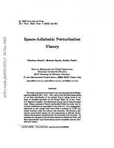
The diagrams contributing to χ at 3 loops are shown in Fig. 2. Absent from this list are circa 140 diagrams involving the 2-point vertex of QL as well as the effective vertex of Fig. 1c, since both these vertices vanish in the case of zero external momentum (provided no infrared divergences are generated in this case, which we explicitly check). γ) From an algorithmic point of view, the contraction for a given diagram entails the following: i) For each vertex involved, look up the corresponding expression for V and symmetrize it partially, according to the incidence matrix; thus, if two vertices are connected by n lines (bij =n), only one of the two need be symmetrized with respect to those lines. In a diagram like that of Fig. 2k, this means a potential saving of a factor of 4! in memory for intermediate expressions. Similar considerations apply for ei ≥ 2 and bii ≥ 4. ii) Form the product of all partially symmetrized vertices, renaming all indices (and momenta) as follows: Indices assigned to contracted legs become internal (µi →ρi′ , aj →cj ′ , kk →pk′ ), and both internal and external indices are placed in ascending order, so as to make sure that their names remain distinct. iii) For each element of bij (i>j) consider in pairs the first bij available powers of the gauge c

field from the ith and the jth vertex (say, Acρii (pi ) and Aρjj (pj )) and substitute them with the propagator:
1 (2π)4 pi,ρi pˆj,ρj δ(pi +pj ) δci cj 2 2 pˆ2i δρi ρj − (1 − α)ˆ 4 a (ˆ pi ) i pi ρi

( pˆi,ρi = e

− 1,

pˆ2i

=

4 X

(2.10)

pˆi,ρ pˆ∗i,ρ )

ρ=1

Similarly for self-contractions (bii ≥ 2).

iv) Simplify color structures. Using the identity: 1 1 a Tija Tkl = δil δkj − δij δkl (2.11) 2 2N (valid for SU (N )), all internal color indices are completely eliminated. The algorithms which implement this simplification are identical to the ones used in the continuum [15]. v) Eliminate all Kronecker δ’s involving internal Lorentz indices. Doing so requires a judicious partial expansion of the expression (which is a product of large sums), to avoid drastic increases in memory. 7

vi) Compactify the expression using the symmetry under permutations of the names of internal momenta and Lorentz indices. Allowed permutations for momenta are those consistent with the topology of the corresponding diagram, that is, permutations which leave invariant the momentum conservation delta functions δ(p1 + · · · +pn ) (or exp ix·(p1 + · · · +pn )) at each vertex; a table of these permutations is constructed right from the beginning. A conceptually easy algorithm would now generate all permuted versions of each subexpression and then select the first version in some order (e.g. lexicographic). The problem is that both intermediate memory and execution time will grow factorially with the number of indices; since we often encounter up to ten indices, already at three loops, it is clear that such an algorithm will not do. At the price of a rather complicated source code, we have come up with an ordering algorithm which is (quasi-)polynomial in nature. Other considerations made here are ordering momenta simultaneously with indices, and casting our expressions in a form involving at most four Lorentz indices (given that the theory is defined in four dimensions). vii) Finally, trigonometric simplifications are systematically performed throughout, in order to put all terms in a canonical form, which then makes identifications or cancellations automatic.

δ) Extracting the analytic, exact momentum dependence of an n-point function, in the limit a→0, is one of the most complicated tasks, both conceptually and algorithmically. This task does not enter the calculation which we present here; its elaboration is still in progress, and will be essential for the calculation of multiplicative renormalizations. Even in continuum regularizations this problem is only completely resolved at one loop [16], [17]. To arbitrary loops, no systematic analysis of n-point functions exists. On the lattice, the first step is to decompose a given expression (to be integrated over internal momenta) in terms of a limited set of potentially divergent integrands, plus other terms which can be evaluated by setting the external momenta directly to zero. A possible basis for this set is:

Qn Q4 i=1

µ=1 (sin piµ ) Qn p2i ) i=1 (ˆ

αiµ

,

8

0 ≤ αiµ ≤ αmax iµ

(2.12)

This decomposition poses no conceptual difficulty, but can cause disproportionate increases in memory, unless it is carefully implemented. One must now integrate the above set, expressing the result in terms of standard functions (logarithms, Spence functions, etc.) and numerical constants characteristic of the lattice. At one loop this has been done systematically [18], using a dimensional regularization technique [19]. At higher loops, not only do these integrals become quite complicated, but their number also grows significantly. We are presently developing algorithms for carrying out the integration of the basis functions (2.12) symbolically. ǫ) Having arrived this far, the only remaining task is the numerical evaluation of loop integrals with no dependence on external momenta. We do this both for finite and infinite lattices. On a finite lattice, loop integrals become nested multiple sums (with due attention paid to propagator zero modes). A mere conversion of the integrand to Fortran or C syntax is almost immediate. However, to produce optimized code one must take into account the following factors: i) Under certain changes of variables ({piµ ↔piν , ∀i}, {piµ →−piµ , ∀i}, etc.) the integrand stays invariant (or can be rendered invariant at a small expense in size). It thus suffices to integrate over a small hypertriangular region of the original domain {−π ≤ piµ ≤ π, ∀i, µ}. An added complication for finite lattices is that the boundaries of this region are sets of nonzero measure. ii) Most diagrams contain two or more loops with no propagator line in common. (Among three loop diagrams the ‘Mercedes’, Fig. 2f, is the only exception.) Integration over the corresponding loop momenta need not be nested, but can be done independently, since all denominators (propagators) can be factorized into terms containing at most one such momentum. In order to factorize numerators as well, one must expand trigonometric functions containing more than one of the above loop momenta (again, our algorithms are written with an eye on keeping expansions to a minimum). The computational load for the resulting code is comparable to that of lower loop integrals. iii) The trigonometric functions comprising each monomial in the integrand typically depend only on a very small subset of the integration variables and can thus be pulled 9

out of most nested integrals. Further, since such factors are shared among many monomials, one can organize them in an (inverse!) tree, to avoid redundant integrations. We have incorporated all the above considerations in an algorithm which takes an integrand as input and produces optimized Fortran code for its integration. For lattice sizes of interest (∼164 ), this optimization results in a gain in execution time of a factor of 107 ! On infinite lattices, a drastic optimization is achieved by putting all propagators in the Schwinger representation:

Z ∞ 1 −αi pˆ2i = e dαi (2.13) pˆ2i 0 In this representation, integrations over different spatial directions factorize, so that their effective number is reduced by 3L−P (L: # of loops, P : # of propagators). At least one of the remaining integrations can be done analytically in terms of Bessel functions, leaving fewer integrals to be done numerically and a less singular integrand. We illustrate this with a very simple example: Z ∞ Z +π 1 d4 p d4 q I≡ dα1 dα2 dα3 e−8(α1 +α2 +α3 ) Φ4 (α1 , α2 , α3) 2 (2π)4 (2π)4 = 2 2 d 0 −π p ˆ qˆ p+q Z +π dp dq exp(2α1 cos p + 2α2 cos q + 2α3 cos(p+q)) Φ(α1 , α2, α3 ) = 2 −π (2π) Z +π q dp 2α2 cos p = e I0 (2 α21 +α23 +2α1 α3 cos p) −π 2π

(2.14)

(2.15)

(I0 is the modified Bessel function.) The resulting expressions are amenable to highprecision Gauss-Legendre type integration. We also compare results for the infinite lattice to an extrapolation of finite lattice (L4 ) results, of the form: B (2.16) Ln In addition to A and B, the exponent n may also vary for different diagrams (and one may result(L) = A +

also expect logarithms of L, cf. Ref. 20). The discrepancy between this extrapolation and the infinite lattice result is typically a fraction of one per mille. In Table I we present the results for each diagram contributing to d4 , for lattices of different size. Adding up all the contributions, we obtain for d4 (on an infinite lattice): d4 = N 4 (N 2 − 1) (1.735N 2 − 10.82 + 73.83/N 2 ) 10−7 10

(2.17)

Our programs are implemented in the computer language Mathematica. All numerical computations are performed by separate Fortran programs generated by our Mathematica routines. The generation of all vertices of QL with up to six legs (needed for the two-loop calculation of Z(β)) requires approximately 30 hours on a SUN Sparc Station 2 with 32 Mbytes of RAM. The computation has to be split into ∼ 200 independently computed contributions (summed only at the very end) in order to fit intermediate results into available RAM.

3.

Results and Conclusions

The value obtained for d4 allows one in principle to extract χ with greater precision. With this value and those previously obtained for d3 we have performed a series of best fits of Eq. (2.4) to Monte Carlo data for SU (2) and SU (3). As in Refs. [7], [8] we have neglected the mixing with hF F i. The values obtained for χu (the non-renormalized topological susceptibility, χu =χ Z 2 (β)) are shown in Table II. They are in good agreement with those of Refs. [7], [8] (q.v. for details). At this stage, increased statistics of Monte Carlo data would be quite welcome on three counts: Improving the estimate of χ, assessing the importance of the hF F i mixing, and checking for nonperturbative contributions in dn (such contributions are possible only for sufficiently high n, cf. Ref. 21). In conclusion, the calculational scheme which we have developed allows us to perform lattice perturbative calculations automatically, with very little ‘human intervention’. Our aim is to be able to repeat the computation for different lattice operators without further programming, and this has not yet been completely achieved. The greatest difficulty that had to be overcome was the existing constraints on computer time and memory, which necessitate devising polynomial-type algorithms and optimizing every aspect of this scheme. One major task still left open is the algorithmic extraction of external momentum dependence. Our first original application was the evaluation to 3 loops of the perturbative tail of χ. We have also obtained three loop results for the gluonic condensate, and report them in a forthcoming publication [22]. Repeating these calculations in the presence of dynamical fermions is relatively straightforward: Only a few additional diagrams appear, requiring no further computational resources. The calculation of multiplicative renormalizations within 11

this scheme, as well as a technical description of our algorithms, are postponed to a future publication. Acknowledgements. It is a pleasure to thank Adriano Di Giacomo for many useful conversations. We acknowledge financial support from MURST (Italian Ministry of the University and of Scientific and Technological Research) and from the Spanish-Italian “Integrated Action” (contract A17). B.A. also acknowledges a Spanish CICYT contract.

12

References 1. G. ’t Hooft, Phys. Rev. Lett. 37 (1976) 8; Phys. Rev. D14 (1976) 3432. 2. E. Witten, Nucl. Phys. B156 (1979) 269. 3. G. Veneziano, Nucl. Phys. B159 (1979) 213. 4. R. J. Crewther, La Rivista del Nuovo Cimento, serie 3, Vol. 2, 8 (1979). 5. P. Di Vecchia, K. Fabricius, G. C. Rossi and G. Veneziano, Nucl. Phys. B192 (1981) 392; Phys. Lett. 108B (1982) 323. 6. M. Campostrini, A. Di Giacomo, H. Panagopoulos, Phys. Lett.212B (1988) 206. 7. M. Campostrini, A. Di Giacomo, H. Panagopoulos, E. Vicari, Nucl. Phys. B329 (1990) 683. 8. M. Campostrini, A. Di Giacomo, Y. G¨ und¨ uc., M. P. Lombardo, H. Panagopoulos, R. Tripiccione, Phys. Lett. B252 (1990) 436. 9. M. Teper, Nucl. Phys. B (Proc. Suppl.) 20 (1991) 159, and references therein. 10. K. Bitar et al., Nucl. Phys. B (Proc. Suppl.) 20 (1991) 390. 11. B. All´es, A. Di Giacomo, Phys. Lett. B294 (1992) 269. 12. A. Di Giacomo, E. Meggiolaro, H. Panagopoulos, Phys. Lett. B277 (1992) 491. 13. M. Campostrini, P. Rossi, Phys. Lett. 242B (1990) 81. 14. B. All´es, M. Giannetti, Phys. Rev. D44 (1991) 513. 15. P. Cvitanovic, Phys. Rev. D14 (1976) 1536. 16. G. ’t Hooft, M. Veltman, Nucl. Phys. B153 (1979) 365. 17. G. Passarino, M. Veltman, Nucl. Phys. B160 (1979) 151. 18. H. Panagopoulos, E. Vicari, Nucl. Phys. B332 (1990) 261. 19. H. Kawai, R. Nakayama, K. Seo, Nucl. Phys. B189 (1981) 40. 20. M. L¨ uscher, P. Weisz, Nucl. Phys. B266 (1986) 309. 21. V. A. Novikov, M. A. Shifman, A. I. Vainshtein, V. I. Zakharov, Nucl. Phys. B174 (1980) 378; 237 (1984) 525; 249 (1985) 445. 22. B. All´es, M. Campostrini, A. Feo, H. Panagopoulos, The Three-Loop Lattice Free Energy, Pisa preprint IFUP-TH 32/92. 13

Table I We list here the contribution to d4 of individual diagrams, shown in Fig. 2, in the Feynman gauge. We use an L4 lattice and gauge group SU(N). Each entry must be multiplied by N 6 (N 2 − 1) ×10−7 . Fig.

L=3

L=8

L = 16

L=∞

a

31.23−33.75/N 2

37.79−41.25/N 2

37.79−41.38/N 2

37.77−41.40/N 2

b

−2.137

−2.981

−3.081

−3.114

c+d

5.210

10.07

10.78

11.02

e

−4.328

−5.964

−6.162

−6.228

f

.3955

.7233

.7429

.7457

g

.0882

.3107

.3100

.3099

h

1.988

1.063

.8017

.7082

i+j

0

9.242 ×10−6

9.112 ×10−6

9.109 ×10−6

k

12.36−18.85/N 2

17.06−24.49/N 2

17.56−24.60/N 2

17.73−24.61/N 2

+56.56/N 4

+73.48/N 4

+73.81/N 4

+73.83/N 4

−44.09+44.99/N 2

−56.37+55.00/N 2

−57.02+55.17/N 2

−57.20+55.18/N 2

l

Table II We list the values of χu /Λ4QCD (for gauge groups SU (2) and SU (3), as obtained from Eq. (2.4) and Monte Carlo data [7], [8] through a series of fits, in which: a) d4 was an additional parameter to be fitted, or: b) the exact value of d4 was taken from our calculation, fitting instead d5 . χu /Λ4QCD

SU (2)

SU (3)

a

2.35(22) 104

2.58(64) 105

b

2.07(23) 104

2.70(69) 105

14

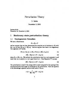
a)

b)

c)

Fig. 1 Effective vertices. Solid (dashed) lines represent gluons (ghosts). Bullets are insertions of Q.

a)

i)

b)

c)

d)

f)

g)

h)

j)

k)

e)

l)

Fig. 2 Diagrams contributing to d . A cross 4 stands for the integration measure.

15