Lattice Reduction for Modular Knapsackâ. Thomas Plantard, Willy Susilo, and Zhenfei Zhang. Centre for Computer and Information Security Research. School of ...
Lattice Reduction for Modular Knapsack? Thomas Plantard, Willy Susilo, and Zhenfei Zhang Centre for Computer and Information Security Research School of Computer Science & Software Engineering (SCSSE) University Of Wollongong, Australia {thomaspl, wsusilo, zz920}@uow.edu.au
Abstract. In this paper, we present a new methodology to adapt any kind of lattice reduction algorithms to deal with the modular knapsack problem. In general, the modular knapsack problem can be solved using a lattice reduction algorithm, when its density is low. The complexity of lattice reduction algorithms to solve those problems is upper-bounded in the function of the lattice dimension and the maximum norm of the input basis. In the case of a low density modular knapsack-type basis, the weight of maximum norm is mainly from its first column. Therefore, by distributing the weight into multiple columns, we are able to reduce the maximum norm of the input basis. Consequently, the upper bound of the time complexity is reduced. To show the advantage of our methodology, we apply our idea over the floating-point LLL (L2 ) algorithm. We bring the complexity from O(d3+ε β 2 + d4+ε β) to O(d2+ε β 2 + d4+ε β) for ε < 1 for the low density knapsack problem, assuming a uniform distribution, where d is the dimension of the lattice, β is the bit length of the maximum norm of knapsack-type basis. We also provide some techniques when dealing with a principal ideal lattice basis, which can be seen as a special case of a low density modular knapsack-type basis.
Keywords: Lattice Theory, Lattice Reduction, Knapsack Problem, LLL, Recursive Reduction, Ideal Lattice.
1
Introduction
To find the shortest non-zero vector within an arbitrary lattice is an NPhard problem [1]. Moreover, till now there is no polynomial algorithm that finds a vector in the lattice that is polynomially close to the shortest non-zero vector. However, there exist several algorithms, for example, LLL [14] and L2 [19], running in polynomial time in d and β, where d is the dimension of the lattice, and β is the bit length of the maximum norm ?
This work is supported by ARC Future Fellowship FT0991397.
2
Thomas Plantard, Willy Susilo, and Zhenfei Zhang
of input basis, that find vectors with exponential approximation (in d) to the shortest non-zero vector. Indeed, in some lattice based cryptography/cryptanalysis, it may not be necessary to recover the exact shortest non-zero vector, nor a polynomially close one. Finding one with exponential distance to the shortest one is already useful, for instance, to solve a low density knapsack problem or a low density modular knapsack problem. Definition 1 (Knapsack P Problem). Let {X1 , X2 , . . . , Xd } be a set of positive integers. Let c = d1 si Xi , where si ∈ {0, 1}. A knapsack problem is given {Xi } and c, find each si . The density of a knapsack, denoted by ρ, is d/β, where β is the maximum bit length of Xi -s. Definition 2 (Modular KnapsackPProblem). Let {X0 , X1 , . . . , Xd } be a set of positive integers. Let c = d1 si Xi mod X0 , where si ∈ {0, 1}. A modular knapsack problem is given {Xi } and c, find each si . ThePknapsack problem is also known as the subset sum problem [12]. When si � d, it becomes a sparse subset sum problem (SSSP). The decisional version of the knapsack problem is NP-complete [9]. However, if its density is too low, there is an efficient reduction to the problem of finding the shortest vector from a lattice (refer to [13, 21, 3]). In this paper, we deal with a (modular) knapsack problem assuming a uniform distribution, i.e., Xi -s are uniformly randomly distributed. We refer to BK as the knapsack-type basis, and BM as the modular knapsack-type basis. In the rest of the paper, for simplicity, we focus on knapsack-type basis, although the adoption over a modular knapsack-type basis is straightforward. X1 1 0 . . . 0 X0 0 0 . . . 0 X2 0 1 . . . 0 X1 1 0 . . . 0 X3 0 0 . . . 0 BK = BM = X2 0 1 . . . 0 . , .. .. .. . . .. .. .. .. . . .. . . . . . . . . . . Xd 0 0 . . . 1
Xd 0 0 . . . 1
We also consider a principal ideal lattice basis. A principal ideal lattice is an ideal lattice that can be represented by two integers. This type of lattice enables important applications, for instance, constructing fully homomorphic encryption schemes with smaller key size (see [5, 26] for an example of this optimization).
Lattice Reduction for Modular Knapsack
3
A basis of a principal ideal lattice (see Section 5) maintains a similar form of modular knapsack basis, with Xi = −αi mod X0 for i ≥ 1, where α is the root for the principal ideal. The security of the corresponding cryptosystem is based on the complexity of reducing this basis. In general, to solve any of the above problems using lattice, one always start by performing an LLL reduction on a lattice L(BK ) (L(BM ), respectively). Then depending on the type of problem and the result the LLL algorithm produces, one may perform stronger lattice reduction (BKZ [24, 7, 2] for example) and/or use enumeration techniques such as Kannan SVP solver [8]. To date, the complexity of best LLL reduction algorithms for the above three type of basis is upper bounded by O(d3+ε β 2 + d4+ε β) [19], although heuristically, one is able to obtain O(d2+ε β 2 ) in practice when ρ is significantly smaller than 1 [20]. Our Contribution: We propose a new methodology to reduce low density modular knapsack-type basis using LLL-type algorithms. Instead of reducing the whole knapsack-type basis directly, we pre-process its sub-lattices, and therefore, the weight of Xi -s is equally distributed into several columns and the reduction complexity is thereafter reduced. Although the idea is somewhat straightforward, the improvement is very significant. Algorithms Time Complexity LLL[14] LLL for knapsack L2 [19] L2 for knapsack[19] ˜ 1 [22] L
O(d5+ε β 2+ε ) O(d4+ε β 2+ε ) O(d4+ε β 2 + d5+ε β) O(d3+ε β 2 + d4+ε β) O(dω+1+ε β 1+ε + d5+ε β)
Our rec-L2 O(d2+ε β 2 + d4+ε β) ˜ 1 O(dω β 1+ε + d4+ε β) Our rec-L
Table 1: Comparison of time complexity
Table 1 shows a time complexity comparison between our algorithms and the existing algorithms. However, we note that the complexities of all the existing algorithms are in worst-case, or in another words, for any type of basis, the algorithms will terminate in the corresponding time. In contrast, in our algorithm, we assume a uniform distribution, and therefore, the complexity given for our recursive reduction algorithms is
4
Thomas Plantard, Willy Susilo, and Zhenfei Zhang
the upper bound following this assumption. Nevertheless, we note that such an assumption is quite natural in practice. Our result is also applicable to a principal ideal lattice basis. In addition, we provide a technique that further reduces the time complexity. Note that our technique does not affect the asymptotic complexity as displayed in Table 1. Paper Organization: In the next section, we review some related area to this research. In Section 3, we propose our methodology to deal with low density knapsack-type basis, introduce our recursive reduction algorithm, and analyze its complexity. Then, we apply our method to L2 and compare its complexity with non-modified L2 in Section 4. In Section 5, we analyze the special case of the principal ideal lattice basis. Finally, the last section concludes this paper.
2 2.1
Background Lattice Basics
In this subsection, we review some concepts of the lattice theory that will be used throughout this paper. The lattice theory, also known as the geometry of numbers, was introduced by Minkowski in 1896 [17]. We refer readers to [15, 16] for a more complex account. Definition 3 (Lattice). A lattice L is a discrete sub-group of Rn , or equivalently the set of all the integral combinations of d ≤ n linearly independent vectors over R. L = Zb1 + Zb2 + · · · + Zbd , bi ∈ Rn B = (b1 , . . . , bd ) is called a basis of L and d is the dimension of L, denoted as dim(L). L is a full rank lattice if d equals to n. For a given lattice L, there exists an infinite number of basis. However, its determinant (see Definition 4) is unique. Definition 4 (Determinant). Let L be a lattice. Its determinant, denoted as det(L), is a real value, such that for any basis B of L, det(L) = p det(B · B T ), where B T is the transpose of B. Definition 5 (Successive Minima). Let L be an integer lattice of dimension d. Let i be a positive integer. The i-th successive minima with
Lattice Reduction for Modular Knapsack
5
respect to L, denoted by λi , is the smallest real number, such that there exist i non-zero linear independent vectors ~v1 , ~v2 , . . . , ~vi ∈ L with kv1 k, kv2 k, . . . , k~vi k ≤ λi . The i-th minima of a random lattice (as defined in Theorem 1) is estimated by: r 1 d λi (L) ∼ det(L) d . (1) 2πe Definition 6 (Hermite Factor). Let B = (b1 , . . . , bd ) a basis of L. The Hermite factor with respect to B, denoted by γ(B), is defined as kb1 k 1 . det(L) d
Note that Hermite factor indicates the quality of a reduced basis. Additionally, following the result of [6]: Theorem 1 (Random Lattice). Let B be a modular knapsack-type basis constructing from a modular knapsack problem given by {Xi }. L(B) is a random lattice, if {Xi } are uniformly distributed.
2.2
Lattice Reduction Algorithms
In 1982, Lenstra, Lenstra and Lovasz [14] proposed an algorithm, known as LLL, that produces an LLL-reduced basis for a given basis. For a lattice L with dimension d, and a basis B, where the norm of all spanning vectors in B is ≤ 2β , the worst-case time complexity is polynomial O(d5+ε β 2+ε ). Moreover, it is observed in [20] that in practice, LLL seems to be much more efficient in terms of average time complexity. In 2005, Nguyen and Stehl´e [19] proposed an improvement of LLL, which is the first variant whose worst-case time complexity is quadratic with respect to β. This algorithm is therefore named L2 . This algorithm makes use of floating-point arithmetics, hence, the library that implements L2 is sometimes referred to as fplll [23]. It terminates with a worstcase time complexity of O(d4+ε β 2 + d5+ε β) for any basis. For a knapsacktype basis, it is proved that L2 terminates in O(d3+ε β 2 + d4+ε β), since there are O(dβ) loop iterations for these bases instead of O(d2 β) for random bases (see Remark 3, [19]). Moreover, some heuristic results show that when dealing with this kind of bases, and when d, β grow to infinity, one obtains Θ(d3 β 2 ) when β = Ω(d2 ), and Θ(d2 β 2 ) when β is significantly larger than d (see Heuristic 3, [20]).
6
Thomas Plantard, Willy Susilo, and Zhenfei Zhang
Recently, in 2011, Novocin, Stehl´e and Villard [22] proposed a new improved LLL-type algorithm that is quasi-linear in β. This led to the ˜ 1 . It is guaranteed to terminate in time O(d5+ε β + dω+1+ε β 1+ε ) name L for any basis, where ω is a valid exponent from matrix multiplications. To bound ω, we have 2 < ω ≤ 3. A typical setting in [22] is ω = 2.3. In [27], van Hoeij and Novocin proposed a gradual sub-lattice reductions algorithm based on LLL that deals with knapsack-type basis. Unlike other LLL-type reduction algorithms, it only produces a basis of a sublattice. This algorithm uses a worst-case O(d7 + d3 β 2 ) time complexity. For more improvements on LLL with respect to d, we refer readers to [18, 25, 10, 11]. With regard to the quality of a reduced basis for an arbitrary lattice, the following theorem provides an upper bound. Theorem 2. For a lattice L, if (b1 , . . . , bn ) form an LLL-reduced basis of L, then, d−1 ∀i, kbi k ≤ 2 2 max(λi (L)). (2) Therefore, assuming a uniform distribution, we have the following. 1. If a modular knapsack problem follows a uniform distribution, then its corresponding basis forms a random lattice. 2. If L is a random lattice, then λi (L) is with respect q to Equation 1.
3. From Equation 1 and 2, we have kbi k ≤ 2 random lattice.
d−1 2
d 2πe
1
det(L) d for a
Hence, for a modular knapsack-type basis, if B = (b1 , . . . , bd ) forms its LLL-reduced basis, then 1
kbi k < 2d det(L) d ,
1 ≤ i ≤ d.
In terms of the quality of kb1 k, the work in [4] shows that on average cases, LLL-type reduction algorithms is able to find a short vector with a Hermite factor 1.0219d , while on worst cases, 1.0754d , respectively. Further, heuristically, it is impossible to find vectors with Hermite factor < 1.01d using LLL-type algorithms [4]. By contrast, a recent work of BKZ 2.0 [2] finds a vector with a Hermite factor as small as 1.0099d . It has been shown that other lattice reduction algorithms, for instance, BKZ [24, 7], and BKZ 2.0 [2], produce a basis with better quality. However, in general, they are too expensive to use. We also note those methods require to perform at least one LLL reduction. As for low density knapsack-type basis, the Hermite factor of the basis is large. This implies that, in general, the output basis of most reduction
Lattice Reduction for Modular Knapsack
7
algorithms contains the demanded short vector. In this case, the time complexity is more important, compared with the quality of the reduced basis/vectors. For this reason, in this paper, we focus only on LLL-type reduction algorithms.
3 3.1
Our Reduction Methodology A Methodology for Lattice Reduction
In this subsection, we do not propose an algorithm for lattice reduction but rather a methodology applicable to all lattice reduction algorithms for the knapsack problem with uniform distribution. Let A be an LLL-type reduction algorithm that returns an LLLreduced basis Bred of a lattice L of dimension d, where Bred = (b1 , . . . , bd ), 1 0 < kbi k < cd0 det(L) d for certain constant c0 . The running time will be c1 da1 β b1 + c2 da2 β b2 , where a1 , b1 , a2 and b2 are all parameters, c1 and c2 are two constants. Without losing generality, assuming a1 ≥ a2 , b1 ≤ b2 (if not, then one term will overwhelm the other, and hence, making the other term negligible). We note that this is a formalization of all LLL-type reduction algorithms. For a knapsack-type basis B of L, where most of the weight of β are from the first column of the basis matrix B = (b1 , b2 , . . . , bd ), it holds that 2β ∼ det(L). Moreover, for any sub-lattice Ls of L that is spanned by a subset of row vectors {b1 , b2 , . . . , bd }, it is easy to prove that det(Ls ) ∼ 2β . In addition, since we assume a uniform distribution, the sub-lattice spanned by the subset of vectors can be seen as a random lattice. Note that the bases of those sub-lattice are knapsack-type basis, so if one needs to ensure the randomness, one is required to add a new vector hX0 , 0, . . . , 0i to the basis and convert it to a modular one. One can verify that this modification will not change the asymptotic complexity. Nevertheless, in practice, it is natural to omit this procedure. We firstly pre-process the basis, so that the weight is as equally distributed into all columns as possible, and therefore, the maximum norm of the new basis is reduced. Suppose we cut the basis into d/k blocks and each block contains k vectors. Then one applies A on each block. Since we know that the determinant of each block is ∼ 2β , this pre-processing gives us a basis with smaller maximum norm ∼ ck0 2β/k . Further, since the pre-processed basis and the initial basis span the same lattice, the preprocessing will not affect the quality of reduced basis that a reduction algorithm returns.
8
Thomas Plantard, Willy Susilo, and Zhenfei Zhang
Below, we show an example of how this methodology works with dimension 4 knapsack-type basis, where we cut L into two sub-lattices and β pre-process them independently. As a result, Xi ∼ 2β , while xi,j . c20 2 2 for a classic LLL-type reduction algorithm. X1 1 0 0 0 x1,1 x1,2 x1,3 0 0 X2 0 1 0 0 x2,1 x2,2 x2,3 0 0 Bbef ore = X3 0 0 1 0 =⇒ Baf ter = x3,1 0 0 x3,4 x3,5 X4 0 0 0 1 x4,1 0 0 x4,4 x4,5 Now we examine the complexity. The total time complexity of this preprocessing is c1 dk a1 −1 β b1 + c2 dk a2 −1 β b2 . The complexity of the final reduction now becomes c1 da1 (k log2 (c0 )+β/k)b1 +c2 da2 (k log2 (c0 )+β/k)b2 . Therefore, as long as c1 da1 (k log2 (c0 ) + β/k)b1 + c2 da2 (k log2 (c0 ) + β/k)b2 +c1 dk
a1 −1 b1
β
+ c2 dk
a2 −1 b2
β
a1 b1
< c1 d β
(3) a2 b2
+ c2 d β ,
conducting the pre-processing will reduce the complexity of whole reduction. In the case where k log2 (c0 ) is negligible compared with β/k, we obtain: c1 da1 (β/k)b1 + c2 da2 (β/k)b2 + c1 dk a1 −1 β b1 + c2 dk a2 −1 β b2 < c1 da1 β b1 + c2 da2 β b2 . Therefore, � � � � da2 da1 c1 da1 − b1 − dk a1 −1 β b1 +c2 da2 − b2 − dk a2 −1 β b2 > 0. k k Taking L2 as an example, where a1 = 4, b1 = 2, a2 = 5 and b2 = 1, let 15 5 k = d/2, we obtain c1 ( 87 d4 − 4d2 )β 2 + c2 ( 16 d − 2d4 )β from the left hand side, which is positive for dimension d > 2. This indicates that, in theory, when dealing with a knapsack-type basis, one can always achieve a better complexity by cutting the basis into two halves and pre-process them independently. This leads to the recursive reduction in the next section. 3.2
Recursive Reduction with LLL-type Algorithms
The main idea is to apply our methodology to an input basis recursively, until one arrives to sub-lattice basis with dimension 2. In doing so, we
Lattice Reduction for Modular Knapsack
9
achieve a upper bounded complexity of O(da1 −b1 β b1 + da2 −b2 β b2 ). For simplicity, we deal with lattice whose dimension equals to a power of 2, although same principle is applicable to lattices with arbitrary dimensions.
Algorithm We now describe our recursive reduction algorithm with LLL-type reduction algorithms. Let LLL(·) an LLL reduction algorithm that for any lattice basis B, it returns a reduced basis Br . Algorithm 1 describes our algorithm, where B is a knapsack-type basis of a d-dimensional lattice, and d is a power of 2. Since we have proven that, for any dimension of knapsack-type basis, it is always better to reduce its sub-lattice in advance as long as Equation 3 holds, it is straightforward to draw the following conclusion: the best complexity to reduce a knapsack-type basis with LLL-type reduction algorithms occurs when one cuts the basis recursively until one arrives with dimension 2 sub-lattices.
Algorithm 1 Recursive Reduction with LLL algorithm Input: B, d Output: Br number of rounds ← log2 d Bb ← B for i ← 1 → number of rounds do dim of sublattice ← 2i number of blocks ← d/dim of sublattice Br ← EmptyM atrix() for j ← 1 → number of blocks do Bt ← SubM atrix(Bb , (j − 1) ∗ dim of sublattice + 1, 1, j ∗ dim of sublattice, d) Bt ← LLL(Bt ) Br ← V erticalJoin(Br , Bt ) end for Bb ← Br end for
In Algorithm 1, EmptyM atrix(·) is to generate a 0 by 0 matrix; SubM atrix(B, a, b, c, d) is to extract a matrix from B, starting from ath row and b-th column, finishing at c-th row and d-th column; while V erticalJoin(A, B) is to adjoin two matrix with same number of columns vertically.
10
Thomas Plantard, Willy Susilo, and Zhenfei Zhang
Complexity In the following, we prove that the complexity of our algorithm is O(da1 −b1 β b1 + da2 −b2 β b2 ), assuming ρ < 1. β b1 For the i-th round, to reduce a single block takes c1 2ia1 ( 2i−1 ) + β b2 d ia 2 c2 2 ( 2i−1 ) , while there exist 2i such blocks. Hence, the total complexity is as follows: log2 d � � X d (c1 2ia1 (β/2i−1 )b1 + c2 2ia2 (β/2i−1 )b2 ) 2i i=1
log2 d
=d·
X
(c1 2i(a1 −b1 −1)+b1 β b1 + c2 2i(a2 −b2 −1)+b2 β b2 )
i=1
= c1 2b1 dβ b1
log2 d
X
log2 d
2(a1 −b1 −1)i + c2 2b2 dβ b2
X
i=1
2(a2 −b2 −1)i
i=1
�
�
�
< c1 2b1 dβ b1 2(log2 d+1)(a1 −b1 −1) + c2 2b2 dβ b2 2(log2 d+1)(a2 −b2 −1)
�
< c1 2b1 dβ b1 (2d)a1 −b1 −1 + c2 2b2 dβ b2 (2d)a2 −b2 −1 < c1 2a1 −1 da1 −b1 β b1 + c2 2a2 −1 da2 −b2 β b2 . As a result, we obtain a new time complexity O(da1 −b1 β b1 + da2 −b2 β b2 ).
4
Applying Recursive Reduction to L2
We adapt the classic L2 as an example. The L2 algorithm uses a worstcase complexity of c1 d4 β 2 + c2 d5 β for arbitrary basis. Therefore, applying our recursive methodology, one obtains � �2 � �! log2 d � � X d β β c1 24i + c2 25i 2i 2i−1 2i−1 i=1
log2 d
=
X
(4c1 d2i β 2 + 2c2 d23i β)
i=1
log2 d
= 4c1 dβ 2
X
log2 d
2i + 2c2 dβ
i=1 2
X
23i
i=1 3
< 4c1 dβ (2d) + 2c2 dβ1.15d < 8c1 d2 β 2 + 2.3c2 d4 β.
Now we compare our complexity with the original L2 algorithm. As mentioned earlier, when applying to a knapsack-type basis, the provable
Lattice Reduction for Modular Knapsack
11
worst-case complexity of L2 becomes c1 d3 β 2 + c2 d4 β rather than c1 d4 β 2 + c2 d5 β as for a random basis. However, it is worth pointing out that in practice, one can achieve a much better result than a worst case, since the weight of most Xi is equally distributed into all the columns. Heuristically, one can expect Θ(c1 d2 β 2 ) when d, β go to infinity and β � d. Input a knapsack-type basis, the L2 algorithm (and almost all other LLL-type reduction algorithms) tries to reduce the first k rows, then the k + 1 row, k + 2 row, etc. For a given k + 1 step, the current basis has the following shape: x1,1 x1,2 . . . x1,k+1 0 0 . . . 0 x2,1 x2,2 . . . x2,k+1 0 0 . . . 0 .. .. .. .. .. .. . . ··· . . . · · · . xk,1 xk,2 . . . xk,k+1 0 0 . . . 0 Bknap−L2 = Xk+1 0 . . . 0 1 0 . . . 0 Xk+2 0 . . . 0 0 1 . . . 0 . .. .. .. .. .. . . . ··· . . . · · · . Xd 0 . . . 0 0 0 . . . 1 L2 will reduce the first k + 1 rows during this step. Despite that most β of the entries are with small elements (kxi,j k ∼ O(2 k )), the worse-case complexity of current step still depends on the last row of current step, i.e., hXk+1 , 0, . . . , 0, 1, 0, . . . , 0i. For the recursive reduction, on the final step, the input basis is in the form of: x1,1 x1,2 . . . x1, d +1 0 0 ... 0 2 x2,1 x2,2 . . . x2, d +1 0 0 ... 0 2 .. .. .. .. .. .. . . · · · . . . · · · . xd 0 0 ... 0 2 ,1 xk,2 . . . x d2 , d2 +1 Brec−L2 = x d +1,1 0 . . . 0 x d +1, d +2 x d +1, d +3 . . . x d +1,d+1 2 2 2 2 2 2 x d 2 +2,1 0 . . . 0 x d2 +2, d2 +2 x d2 +2, d2 +3 . . . x d2 +2,d+1 . .. .. .. .. .. .. . ··· . . . ··· . xd,1 0 . . . 0 xd, d +2 xd, d +3 . . . xd,d+1 2
2
Note that the weight of Xi is equally distributed into d2 + 1 columns. Hence, the bit length of maximum norm of basis is reduced from β to approximately d log2 c0 + 2β/d. Therefore, we achieve a better time complexity. In fact, the provable new complexity is of the same level of the heuristic results observed in practice, when β � d.
12
5
Thomas Plantard, Willy Susilo, and Zhenfei Zhang
Special Case: Principal Ideal Lattice Basis
In this section, we present a technique when dealing with a principal ideal lattice basis. Due to the special form of a principal ideal lattice, we are able to reduce the number of reductions in each round to 1, with a cost of O(d) additional vectors for the next round. This technique does not effect the asymptotic complexity, however, in practice, it will accelerate the reduction. δ 0 0 ... 0 δ 0 0 ... 0 0 −α mod δ 1 0 . . . 0 −α 1 0 . . . 0 0 2 BI = −α mod δ 0 1 . . . 0 =⇒ BI0 = 0 −α 1 . . . 0 0 . .. .. .. . . .. .. .. .. .. . . .. . . . . . . . . . . . d−1 0 0 0 . . . −α 1 −α mod δ 0 0 . . . 1 Let X0 = δ, one obtains BI in the above form. From BI , one constructs a new basis BI0 . Then, one can obtain a generator matrix of L(BI ) by inserting some vectors in L to BI0 . The following example shows how to construct G with d = 5. In this example, since vector h0, 0, δ, 0, 0i is a valid vector in L(B), B and G span a same lattice. Applying a lattice reduction algorithm over G will return a matrix with the top row that is a zero vector, while the rest form a reduced basis of L. x1,1 x1,2 x1,3 0 0 δ 0 0 0 0 x2,1 x2,2 x2,3 0 0 −α 1 0 0 0 0 −α 1 0 0 =⇒ x3,1 x3,2 x3,3 0 0 G= 0 0 x1,1 x1,2 x1,3 0 0 δ 0 0 0 0 x2,1 x2,2 x2,3 0 0 −α 1 0 0 0 0 −α 1 0 0 x3,1 x3,2 x3,3 To reduce G, we adopt our recursive reduction methodology. We firstly reduce the top half of G. Since the second half is identical to the top half, except the position of the elements, we do not need to reduce the second half. Indeed, we use the result of the top half block and then shift all the elements. In this case, during our recursive reduction, for round i, instead of doing d/2i reductions, one need to perform only one reduction. Finally, one reduces the final matrix G, removes all the zero vectors and start a new round. With our technique, the number of vectors grows, and this may increase the complexity of the next round. For the i-th round, the number of vectors grows by d/2i−1 − 1. It will be negligible when d/2i � d. For
Lattice Reduction for Modular Knapsack
13
instance, if we adopt this approach between the second last round and the last round, this approach will only increase the number of vectors by 1, while if one uses it prior to the first round, the number of rows will almost be doubled. In practice, one can choose to adopt this technique for each round only when it accelerates the reduction. We note that the asymptotic complexity remains the same, since generally speaking, the number of vectors remains O(d) as before, while the asymptotic complexity concerns only d and β.
6
Conclusion
In this paper, we presented a methodology for lattice reduction algorithms used for solving low density modular knapsack problems. The complexity of polynomial time lattice reduction algorithms relies on the dimension d and the bit length β of maximum norm of input basis. We prove that for a knapsack-type basis, it is always better to pre-process the basis by distributing the weight to many columns as equally as possible. Using this methodology recursively, we are able to reduce β to approximately 2β/d, and consequently, we successfully reduce the entire complexity. We then demonstrated our technique over the floating-point LLL algorithm. We obtain a provable upper bounded complexity of O(d2+ε β 2 + d4+ε β), which is by far the best provable time complexity for a knapsacktype basis.
References 1. M. Ajtai. The shortest vector problem in l2 is NP-hard for randomized reductions (extended abstract). In Thirtieth Annual ACM Symposium on the Theory of Computing (STOC 1998), pages 10–19, 1998. 2. Y. Chen and P. Q. Nguyen. BKZ 2.0: Better lattice security estimates. In D. H. Lee and X. Wang, editors, ASIACRYPT, volume 7073 of Lecture Notes in Computer Science, pages 1–20. Springer, 2011. 3. M. J. Coster, A. Joux, B. A. LaMacchia, A. M. Odlyzko, C.-P. Schnorr, and J. Stern. Improved low-density subset sum algorithms. Computational Complexity, 2:111–128, 1992. 4. N. Gama and P. Q. Nguyen. Predicting lattice reduction. In Proceedings of the theory and applications of cryptographic techniques 27th annual international conference on Advances in cryptology, EUROCRYPT’08, pages 31–51, Berlin, Heidelberg, 2008. Springer-Verlag. 5. C. Gentry. Fully homomorphic encryption using ideal lattices. In M. Mitzenmacher, editor, STOC, pages 169–178. ACM, 2009. 6. D. Goldstein and A. Mayer. On the equidistribution of Hecke points. In Forum Mathematicum., volume 15, pages 165–189, 2006.
14
Thomas Plantard, Willy Susilo, and Zhenfei Zhang
7. G. Hanrot, X. Pujol, and D. Stehl´e. Analyzing blockwise lattice algorithms using dynamical systems. In P. Rogaway, editor, CRYPTO, volume 6841 of Lecture Notes in Computer Science, pages 447–464. Springer, 2011. 8. R. Kannan. Improved algorithms for integer programming and related lattice problems. In Proceedings of the fifteenth annual ACM symposium on Theory of computing, STOC ’83, pages 193–206, New York, NY, USA, 1983. ACM. 9. R. M. Karp. Reducibility among combinatorial problems. In R. E. Miller and J. W. Thatcher, editors, Complexity of Computer Computations, The IBM Research Symposia Series, pages 85–103. Plenum Press, New York, 1972. 10. H. Koy and C.-P. Schnorr. Segment LLL-reduction of lattice bases. In CaLC, pages 67–80, 2001. 11. H. Koy and C.-P. Schnorr. Segment LLL-reduction with floating point orthogonalization. In CaLC, pages 81–96, 2001. 12. J. C. Lagarias and A. M. Odlyzko. Solving low-density subset sum problems. J. ACM, 32(1):229–246, 1985. 13. M. K. Lai. Knapsack cryptosystems: The past and the future. 2001. 14. A. K. Lenstra, H. W. Lenstra, and L. Lov´ asz. Factoring polynomials with rational coefficients. Mathematische Annalen, Springer-Verlag, 261:513–534, 1982. 15. L. Lov´ asz. An Algorithmic Theory of Numbers, Graphs and Convexity, volume 50 of CBMS-NSF Regional Conference Series in Applied Mathematics. SIAM Publications, 1986. 16. D. Micciancio and S. Goldwasser. Complexity of Lattice Problems, A Cryptographic Perspective. Kluwer Academic Publishers, 2002. 17. H. Minkowski. Geometrie der Zahlen. B. G. Teubner, Leipzig, 1896. 18. I. Morel, D. Stehl´e, and G. Villard. H-LLL: using householder inside LLL. In ISSAC, pages 271–278, 2009. 19. P. Q. Nguyen and D. Stehl´e. Floating-point LLL revisited. In Advances in Cryptology - Eurocrypt 2005, Lecture Notes in Computer Science 3494, Springer-Verlag, pages 215–233, 2005. 20. P. Q. Nguyen and D. Stehl´e. LLL on the average. In 7th International Symposium on Algorithmic Number Theory (ANTS 2006), pages 238–256, 2006. 21. P. Q. Nguyen and J. Stern. Adapting density attacks to low-weight knapsacks. In B. K. Roy, editor, ASIACRYPT, volume 3788 of Lecture Notes in Computer Science, pages 41–58. Springer, 2005. 22. A. Novocin, D. Stehl´e, and G. Villard. An LLL-reduction algorithm with quasilinear time complexity: extended abstract. In L. Fortnow and S. P. Vadhan, editors, STOC, pages 403–412. ACM, 2011. 23. X. Pujol, D. Stehl´e, and D. Cade. fplll library. online. http://perso.ens-lyon. fr/xavier.pujol/fplll/. 24. C.-P. Schnorr. A more efficient algorithm for lattice basis reduction. J. Algorithms, 9(1):47–62, 1988. 25. C.-P. Schnorr. Fast LLL-type lattice reduction. Inf. Comput., 204(1):1–25, 2006. 26. N. P. Smart and F. Vercauteren. Fully homomorphic encryption with relatively small key and ciphertext sizes. In P. Q. Nguyen and D. Pointcheval, editors, Public Key Cryptography, volume 6056 of Lecture Notes in Computer Science, pages 420– 443. Springer, 2010. 27. M. van Hoeij and A. Novocin. Gradual sub-lattice reduction and a new complexity for factoring polynomials. Algorithmica, 63(3):616–633, 2012.