Lattice Study of the Conformal Window in QCD-like Theories

Lattice Study of the Conformal Window in QCD-like Theories Thomas Appelquist, George T. Fleming, and Ethan T. Neil Department of Physics, Sloane Laboratory, Yale University, New Haven, CT, 06520 We study the extent of the conformal window for an SU(3) gauge theory with Nf Dirac fermions in the fundamental representation. We present lattice evidence for 12 ≤ Nf ≤ 16 that the infrared behavior is governed by a fixed point, while confinement and chiral symmetry breaking are present for Nf ≤ 8.

arXiv:0712.0609v2 [hep-ph] 5 May 2008

PACS numbers: 11.10.Hi, 11.15.Ha, 11.25.Hf, 12.60.Nz, 11.30.Qc

With a small number of massless fermions, a vector-like gauge field theory such as QCD exhibits confinement and dynamical chiral symmetry breaking. But if the number of massless fermions, Nf , is larger, near but just below the value, Nfaf , at which asymptotic freedom sets in, the theory is conformal in the infrared, governed by a weak infrared fixed point (IRFP) which appears already in the two-loop beta function [1, 2]. There is no confinement, and chiral symmetry is unbroken. It is thought that this IRFP persists down to some critical value Nfc , where the coupling is sufficiently strong that the transition to the confined, chirally broken phase takes place. The range Nfaf > Nf > Nfc is the “conformal window”, where the theory is in the “nonAbelian Coulomb phase”. Theories in or near the conformal window could play a key role in physics beyond the standard model. For example, a theory near the conformal window could describe electroweak symmetry breaking. It is therefore important to study the extent of this window, as well as the order of the transition at Nfc and the properties of the theory inside the window and near it. Despite interest in these questions for many years, little is known with confidence. This can be contrasted with supersymmetric QCD, where duality arguments determine the extent of the conformal window and lead to weakly coupled effective low-energy theories at both ends [3]. An upper limit on Nfc for both supersymmetric and nonsupersymmetric theories has been proposed based on the counting of massless degrees of freedom, employing the thermodynamic free energy [4]. For a supersymmetric SU(N ) gauge theory with Nf massless Dirac fermions in the fundamental representation (where Nfaf = 3N ), one finds Nfc ≤ (3/2)N , a limit precisely saturated by the result from duality arguments. For a non-supersymmetric SU(N ) theory with Nf massless Dirac fermions in the fundamental representation (where Nfaf = (11/2)N ), one finds Nfc ≤ 4N [1 − (1/18N 2 ) + ...]. It is not known to what extent this limit is saturated. The most recent lattice studies [5], for N = 3, lead the authors to the conclusion that Nfc is much lower. They find 6 < Nfc < 7. In this letter, we describe a new lattice study of the conformal window for an SU(3) gauge theory with Nf Dirac fermions in the fundamental representation. We adopt a gauge-invariant definition of the running coupling, valid

for any strength, derived from the Schr¨odinger functional (SF) of the gauge theory [6, 7, 8]. For an asymptotically free theory, this coupling agrees with the perturbative running coupling at short enough distances [9]. Making use of staggered fermions as in Ref. [10], it is most straightforward to restrict attention to values of Nf that are multiples of 4. The value Nf = 16 leads to an IRFP that is sufficiently weak that it is best studied in perturbation theory. The value Nf = 4 is expected to be well outside the conformal window, leading to confinement and chiral symmetry breaking as with Nf = 2. Thus we focus on Nf = 8 and Nf = 12. The Schr¨odinger functional is the transition amplitude from a prescribed state at time t = 0 to another state at time t = T . It can be written as a Euclidean path integral in a spatial box of size L with Dirichlet boundary conditions at t = 0 and t = T where T is O(L). Periodic boundary conditions are imposed in the spatial direction. The Schr¨odinger functional can be written as Z ′ ′ ′ Z[W, ζ, ζ; W , ζ , ζ ] = [DU DχDχ]e−SG −SF (1) where U are the gauge fields and χ, χ are the staggered fermion fields. W and W ′ are the (fixed) boundary values ′ of the gauge fields, and ζ, ζ, ζ ′ , ζ are the boundary values of the fermion fields at t = 0 and t = T , taken here to be zero. The quantity SG is the Wilson gauge action and SF is the massless staggered fermion action. The gauge boundary values W (η), W ′ (η) are chosen such that the minimum action configuration is a constant chromo-electric field [11, 12] whose magnitude is of O(1/L) and is controlled by a dimensionless parameter η [13]. The SF running coupling g 2 (L, T ) is defined by taking k ∂ , (2) = − log Z 2 ∂η g (L, T ) η=0


L 2 a 2

2

[sin (2πa /3LT ) + sin (πa2 /3LT )] where k = 12 is chosen so that g (L, T ) equals the bare coupling at tree level. In general, g 2 (L, T ) measures the response of the system to small changes in the background chromo-electric field. For staggered fermions, L/a must be even but T /a must be odd, where a is the lattice spacing. To cancel the resultant O(a) bulk lattice artifact, the coupling is defined as the

2 average over T = L ± a:   1 1 1 1 = + . 2 g2 (L, L − a) g2 (L, L + a) g2 (L)

(3)

O(a) terms on the Dirichlet boundaries remain [10]. We include a perturbative one-loop counterterm of O(g04 a) in our calculations to remove partially the O(a) boundary artifact. Since g 2 (L) depends on only one IR scale, L, it provides a technical advantage for studying an IRFP over other possible non-perturbative definitions of the running coupling, such as from the static potential V (r), which must be computed from Wilson loops at scales r ≪ L to avoid finite-size effects [14]. To set the stage, we review briefly the behavior of g 2 (L) in continuum perturbation theory through three loops. By computing g 2 (L) in lattice perturbation theory and setting to zero terms that vanish as a/L → 0, a continuum beta function,
β , may be defined such that L(∂/∂L)g 2 (L) = β g 2 (L) = b1 g4 (L) + b2 g6 (L) + b3 g 8 (L) + · · · , where the first two (scheme-independent) coefficients are     2 2 11 − 23 Nf , b2 = (4π) 102 − 38 Nf . (4) b1 = (4π) 2 4 3 The third coefficient is scheme dependent, given in the SF scheme by [9]

b2 c2 b1 (c3 − c22 ) − , (5) 2π 8π 2 where c2 = 1.256 + 0.040Nf and c3 = c22 + 1.197(10) + 0.140(6)Nf − 0.0330(2)Nf2 , and where bMS 3 is the threeloop coefficient defined in the MS scheme (only in the loop expansion), given by  2857 5033  325 1 2 bMS − N + N . (6) f f 3 = (4π)6 2 18 54 MS bSF 3 = b3 +

For Nf = 16, a weak two-loop IRFP exists at g 2∗ ≃ 0.52. The higher order corrections are very small in both the SF and MS schemes. For Nf = 12, the two- and three-loop beta functions also exhibit an IRFP, although the reliability of the loop expansion is less clear. The two-loop IRFP is at g 2∗ ≃ 9.48. At three loops the fixed point strength is reduced by roughly 50%, to g 2∗ ≃ 5.18 (5.47) in the SF (MS) scheme. (In the MS scheme, where a four-loop result exists, the fixed point value increases slightly to 5.91.) Since the corresponding loop expansion parameter g 2∗ /4π 2 is smaller than unity, perturbation theory could provide a reasonable basis of comparison for our lattice simulations. For Nf = 8, there is no two-loop IRFP. While an IRFP can appear at three loops and beyond, its scheme dependence and typically large value means that there is no evidence for an IRFP accessible in perturbation theory. A non-perturbative study is essential. With this as background, we next describe our lattice simulations for Nf = 8 and 12. For Nf = 8 we compute g 2 (L) for bare lattice couplings β ≡ 6/g02 ∈ [4.5, 7.1] with typically 0.1 spacing. For Nf = 12 we choose

β ∈ [4.15, 6.5] also with typically 0.1 spacing [28]. In both cases, we use lattice extents L/a = 4, 6, 8, 10, 12, 16 and 20, with the larger L/a computations done at fewer β values due to the much higher computational cost. We use the standard hybrid molecular dynamics (HMD) R algorithm [15] with unit length trajectories. We generate three independent ensembles varying the number of steps per trajectory, typically in the range 64–128 steps but up to 512 steps at stronger couplings, and perform a quadratic extrapolation to remove finite step size errors. Within our statistics, the observed systematic shift in g 2 (L) due to finite step size is negligible over the chosen range of step sizes. For the majority of the simulations, those at relatively weak lattice coupling, we employ of order 40,000 HMD trajectories, sufficient to estimate reliably autocorrelations. At stronger couplings, the autocorrelations become much longer, with the time histories showing the previously observed phenomenon [13, 16] of large excursions lasting a few thousand trajectories. In such cases, simulations are run longer, up to 80,000 HMD trajectories. Error estimation is performed using the jacknife method with the block size adjusted to eliminate the effects of autocorrelations. To observe the running of the coupling over a large range of scales requires the generation of several hundred independent ensembles at various values of the box size, L/a, and bare gauge coupling, β ≡ 6/g02 . With so many independent statistical estimates of g 2 (L), occasional large statistical fluctuations of these estimates are expected. So, we model our estimates with a smooth interpolating function based on a truncated Laurent series g2 (β, a/L) =

3 X k=1

ck (a/L) [β − β0 (a/L)]

k

,

(7)

with polynomial dependence of the coefficients on a/L
l
l P2 P2 ck = l=0 ckl La , β0 = l=0 β0l La . (8)

Best-fit values for the coefficients at 8 and 12 flavors will be included in a future paper. This interpolating function is used only to describe the lattice data in the limited range where the data exists, well away from the poles. The extrapolation to the continuum is implemented using the step-scaling procedure [17, 18], a systematic method that captures the renormalization group evolution of the coupling in the continuum limit. The basic idea is to match lattice calculations at different values of a/L, by tuning the lattice coupling β ≡ 6/g02 so that the coupling strength g 2 (L) is equal on each lattice. Keeping g 2 (L) fixed while changing a/L allows one to extract the lattice artifacts. Previous work by the ALPHA collaboration has shown that perturbative counterterms greatly reduce O(a/L) artifacts from the running coupling. So, our preferred method of extrapolating to the continuum limit at each step assumes that O(a2 /L2 ) errors dominate. In practice, one calculates a discretized version of the running coupling, known as the step-scaling function. In

3 16

the continuum, it is designated

σ(s, g 2 (L)) = g 2 (sL),

(9)

14

where s is the step size. On the lattice, a/L terms are also present; one defines Σ(s, g 2 (L), a/L) similarly, so that it reduces to σ(s, g 2 (L)) in the continuum limit:

12

σ(s, g 2 (L)) = lim Σ(s, g2 (L), a/L) a→0

2

(10)

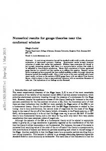
First, a value u = g (L) is chosen. Several ensembles with different values of a/L are then generated, with β ≡ 6/g02 tuned using our interpolating function Eq. (7) so that the measured value of g 2 (L) = u on each. Then for each β , a second ensemble is generated with larger spatial extent, L → sL. The measured value of g 2 (sL) on the larger lattice is exactly Σ(s, u, a/L). Extrapolation in a/L to the continuum then gives us the value of σ(s, u). Using the value of σ(s, u) as the new starting value, this process may then be repeated indefinitely, until we have a series of continuum running couplings with their scale ranging from L to sn L. In this paper, we take s = 2. Our results for Nf = 12 continuum running are presented in Fig. 1. We take L0 to be the scale at which g 2 (L) ≃ 1.6, a relatively weak coupling. The points shown are for values of L/L0 increasing by factors of two. The step-scaling procedure leading to these points involves stepping L/a from 4 → 8, 6 → 12, 8 → 16, and 10 → 20, and then extrapolating Σ(2, u, a/L) to the continuum limit assuming that O(a2 /L2 ) terms dominate. Various sources of systematic error must be accounted for. The interpolating function Eq. (7) may not contain enough terms to capture the true form of g 2 (L) at large L where there is sparse data, and although the O(a/L) terms are expected to be small, ignoring them completely in the continuum extrapolation may introduce a small systematic effect. In addition, a few simulations that had run at least 20% of their target length, but were not yet completed, were included in the fit. The statistical error in g 2 (L) for these cases was likely underestimated. Here we provide an estimate of our systematic error by varying our continuum extrapolation method between extremes. Inspection of Σ(2, u, a/L) as a function of a/L indicates that dropping the step from 4 → 8 and performing a constant extrapolation underestimates the true continuum running, while performing a linear fit to all four steps gives an overestimate. These define the upper and lower bounds of the shaded region in Fig. 1, which we take to be a conservative estimate of the overall systematic error. The observed IRFP for Nf = 12 agrees within the estimated systematic-error band with three-loop perturbation theory in the SF scheme. An important feature for Nf = 12 is that the interpolating curves are anchored by values of g 2 (L) that are also above the IRFP. For β ≤ 4.4, g 2 (L) is large, decreasing as L/a increases with fixed β . In the step-scaling function, values of u in this range lead to Σ(2, u, a/L) < u as a/L → 0. This behavior is similar to that found in Ref. [19] for Nf = 16, and consistent with

2-loop univ. 3-loop SF

10 g 2$L% 8 6 4 2 0

5

10

15 20 Log!L"L0#

25

30

35

FIG. 1: Continuum running coupling from step scaling for Nf = 12. The statistical error on each point is smaller than the size of the symbol. Systematic error is shown in the shaded band.

approaching the IRFP from above in the continuum limit. In a future paper, we will exhibit both the step-scaling results and the continuum evolution in this region. Our results for Nf = 8 continuum running are presented in Fig. 2, starting at a scale L0 where g 2 (L) ≃ 1.6, and exhibiting points with statistical error bars for values of L/L0 increasing by factors of two. The three step-scaling procedures are the same as in the Nf = 12 case. Stepping L/a from 4 → 8, 6 → 12, 8 → 16 and 10 → 20 with quadratic extrapolation again provides the points with statistical error bars, and the other two procedures define the upper and lower bounds of the systematic-error band. For comparison, we have also shown the results of twoand three-loop perturbation theory up to g 2 ≃ 10, beyond which there is no reason to trust the perturbative expansion. The Nf = 8 running coupling shows no evidence for an IRFP, or even an inflection point, up through values exceeding 14. The points with statistical errors begin to increase above three-loop perturbation theory well before this value. This behavior is similar to that found for the quenched theory [20] and for Nf = 2 [16], although, as expected, the rate of increase is slower than in either of these cases. The coupling strength reached for Nf = 8 exceeds rough estimates of the strength required to trigger dynamical chiral symmetry breaking [21, 22, 23], and therefore also confinement. This conclusion must be confirmed by simulations of physical quantities such as the quark-antiquark potential and the chiral condensate at zero temperature. To conclude, we have provided evidence from lattice simulations that for an SU(3) gauge theory with Nf Dirac fermions in the fundamental representation, the value Nf =8 lies outside the conformal window, and therefore leads to confinement and chiral symmetry breaking; while Nf =12 lies within the conformal window, governed by an IRFP. We stress that these conclusions do not depend crucially on the L/a = 4 data, which are of limited use in the SF scheme [6]. Thus the lower end of the conformal

4 16

Simulations were based in part on the MILC code [26], and were performed at Fermilab and Jefferson Lab on clusters provided by the DOE’s U.S. Lattice QCD (USQCD) program, the Yale Life Sciences Computing Center supported under NIH grant RR 19895, the Yale High Performance Computing Center, and on a SiCortex SC648 on loan to Yale from SiCortex, Inc.

2-loop univ.

14

3-loop SF

12 10 2

g $L% 8 6 4 2 0

2

4 6 Log!L"L0#

8

10

FIG. 2: Continuum running coupling from step scaling for Nf = 8. Errors are shown as in Fig. 1. Perturbation theory is shown up to only g 2 (L) ∼ 10.

[1] [2] [3] [4] [5] [6]

window, Nfc , lies in the range 8 < Nfc < 12. This conclusion, in disagreement with Ref. [5], is reached employing the Schr¨odinger functional (SF) running coupling, g 2 (L). This coupling is defined at the box boundary L with a set of special boundary conditions. It runs in accordance with perturbation theory at short enough distances, and is a gauge-invariant quantity that can be used to search for conformal behavior, either perturbative or non-perturbative, in the large L limit. For Nf =8, we have simulated g 2 (L) up to values that exceed rough estimates of the coupling strength required to trigger dynamical chiral symmetry breaking [21, 22, 23, 24], with no evidence for an IRFP. For Nf =12, our observed IRFP is rather weak, agreeing within the estimated errors with three-loop perturbation theory in the SF scheme. The simulations of g 2 (L) at Nf =8 and 12 should be continued to achieve more precision. It is also important to supplement the study of g 2 (L) by examining physical quantities such as the static potential, and demonstrating directly that chiral symmetry is spontaneously broken for Nf =8 through a zero-temperature lattice simulation. Simulations of g 2 (L) for other values of Nf , in particular Nf =10, will be crucial to determine more accurately the lower end of the conformal window and to study the phase transition as a function of Nf . All of these analyses should be extended to other gauge groups and other representation assignments for the fermions [25]. We acknowledge helpful discussions with Urs Heller, Walter Goldberger, Rich Brower, Chris Sachrajda and Aneesh Manohar. This work was supported partially by DOE grant DE-FG02-92ER-40704 (T.A. and E.N.), and took place partly at the Aspen Center for Physics (TA).

[7] [8] [9] [10] [11] [12] [13] [14] [15] [16] [17] [18] [19] [20] [21] [22] [23] [24] [25] [26] [27] [28]

W. E. Caswell, Phys. Rev. Lett. 33, 244 (1974). T. Banks and A. Zaks, Nucl. Phys. B196, 189 (1982). N. Seiberg, Nucl. Phys. B435, 129 (1995). T. Appelquist, A. G. Cohen, and M. Schmaltz, Phys. Rev. D60, 045003 (1999). Y. Iwasaki, K. Kanaya, S. Kaya, S. Sakai, and T. Yoshie, Phys. Rev. D69, 014507 (2004). M. L¨uscher, R. Narayanan, P. Weisz, and U. Wolff, Nucl. Phys. B384, 168 (1992). S. Sint, Nucl. Phys. B421, 135 (1994). A. Bode et al. (ALPHA), Phys. Lett. B515, 49 (2001). A. Bode, P. Weisz, and U. Wolff (ALPHA), Nucl. Phys. B576, 517 (2000), erratum-ibid.B608:481,2001. U. M. Heller, Nucl. Phys. B504, 435 (1997). G. ’t Hooft, Nucl. Phys. B153, 141 (1979). M. L¨uscher, Nucl. Phys. B219, 233 (1983). M. L¨uscher, R. Sommer, P. Weisz, and U. Wolff, Nucl. Phys. B413, 481 (1994). S. Necco and R. Sommer, Nucl. Phys. B622, 328 (2002). S. A. Gottlieb, W. Liu, D. Toussaint, R. L. Renken, and R. L. Sugar, Phys. Rev. D35, 2531 (1987). M. Della Morte et al. (ALPHA), Nucl. Phys. B713, 378 (2005). M. L¨uscher, P. Weisz, and U. Wolff, Nucl. Phys. B359, 221 (1991). S. Caracciolo, R. G. Edwards, S. J. Ferreira, A. Pelissetto, and A. D. Sokal, Phys. Rev. Lett. 74, 2969 (1995). U. M. Heller, Nucl. Phys. Proc. Suppl. 63, 248 (1998). J. Heitger, H. Simma, R. Sommer, and U. Wolff, Nucl. Phys. Proc. Suppl. 106, 859 (2002). T. Appelquist, A. Ratnaweera, J. Terning, and L. C. R. Wijewardhana, Phys. Rev. D58, 105017 (1998). H. Gies and J. Jaeckel, Eur. Phys. J. C46, 433 (2006). E. Gardi and G. Grunberg, JHEP 03, 024 (1999). T. Appelquist and S. B. Selipsky, Phys. Lett. B400, 364 (1997). F. Sannino and K. Tuominen, Phys. Rev. D71, 051901 (2005). C. DeTar et al. (MILC), Version 6. (2002), URL http://www.physics.utah.edu/%7Edetar/milc/. F. R. Brown et al., Phys. Rev. D46, 5655 (1992). In these ranges of bare coupling, we do not observe a bulk phase transition as in Brown et al. [27]