In section 2, we show that Karatsuba's algorithm can actually be made lazy, which leads to the following: Theorem 1. There exists a lazy multiplication al- gorithm ...
Lazy multiplication of formal power series Joris van der Hoeven
Abstract
For most fast algorithms to manipulate formal power series, a fast multiplication algorithm is essential. If one desires to compute all coe�cients of a product of two power series up to a given order, then several e�cient algorithms are available, such as fast Fourier multiplication. However, one often needs a lazy multiplication algorithm, for instance when the product computation is part of the computation of the coe�cients of an implicitly de ned power series. In this paper, we describe two lazy multiplication algorithms, which are faster than the naive method. In particular, we give an algorithm of time complexity O(n log2 n).
Key words: power series, multiplication, algorithm. 1 Introduction
In this paper, we are concerned with fast e�ective computations with power series in z over an e�ective eld of constants C. The time (and space) complexities we consider will be measured in terms of operations on the constants (and the number of constants we need to store). Most known algorithms for fast manipulations of formal power series are based on a fast multiplication algorithm. Since power series are in nite objects, we will be interested in computing the rst (but an arbitrary large number of) coe�cients of them. Now we distinguish two types of multiplication algorithms. First, we have static multiplication algorithms: let f and g be the power series we want to multiply. Then a static multiplication algorithm takes a natural number n and the rst n coe�cients f0 ; � � � ; fn 1; g0; � � � ; gn 1 of f and g on input, and returns the rst n coe�cients
(fg)0 ; � � � ; (fg)n 1 of the product fg. Classical static multiplication algorithms are naive multiplication, Karatsuba's algorithm, and FFT multiplication, of respective complexities O(n2); O(nlog 3= log 2 ) and O(n log n). We refer to [3] for more details. On the other hand, one often needs lazy multiplication algorithms. In this case, the successive coe�cients of f and g are only given one by one, and the lazy multiplication algorithm should output the coe�cient of z i in fg, as soon as f0 ; � � � ; fi ; g0; � � � ; gi are known. The advantage of lazy multiplication is that the coef cients of z i in f and g may be de ned in terms of the rst i coe�cients of fg. For this reason, lazy multiplication can be used as a subalgorithm, when we want to compute the coe�cients of an implicitly de ned power series. An easy example is the exponentiation of a power series h with h0 = 0, which can be computed lazily using the formula Z 0h h e = he : Although the complexity of static multiplication has been studied extensively, the best known bound for lazy multiplication is the naive bound O(n2 ). In section 2, we show that Karatsuba's algorithm can actually be made lazy, which leads to the following:
Theorem 1.
There exists a lazy multiplication algorithm for formal power series, of time complexity O(nlog 3= log 2 ) and space complexity O(n log n).
Let M (n) = n� log n log log n be a complexity bound for the multiplication of two polynomials of degree n 1 and coe�cients in C. In section 3, we prove the main result of this paper:
Theorem 2.
There exists a lazy multiplication algorithm for formal power series, of time complexity O(M (n) log n) and space complexity O(n).
In particular, if C supports FFT multiplication (i.e. the fast Fourier transform), then we may take M (n) =
n log n and we obtain a lazy multiplication algorithm of complexity O(n log2 n). In general, one may take M (N ) = n log n log log n (see [5]). In section 4 we apply theorem 2 to the resolution of implicit equations, and, in this context, we compare the performances of our and more classical algorithms. 2 Karatsuba's multiplication algorithm is lazy Karatsuba's algorithm for polynomials. Let us rst recall Karatsuba's method for multiplying two polynomials P and Q in z of degrees n 1 > 1. We write
P = Plo + Phi z bn=2c Q = Qlo + Qhi z bn=2c ; where the lower parts Plo and Qlo of P resp. Q have degrees 6 bn=2c 1. Then we have PQ = Plo Qlo + ((Plo + Phi )(Qlo + Qhi ) Plo Qlo Phi Qhi )z bn=2c + Phi Qhi z 2bn=2c: Karatsuba's algorithm consists of recursively applying the above formula in order to compute the product PQ. Since the multiplication of two polynomials of degree n 1 involves only three multiplications of polynomials of degrees 6 bn=2c, the asymptotic time complexity of the method is O(nlog 3= log 2). Important observation. If we apply the above algorithm symbolically to compute a formula for (PQ)i, then we notice that this only depends on the coe�cients P0 ;� � �;Pi and Q0 ; � � � ; Qi. Actually, this observation implies at once the existence of a lazy version of Karatsuba's algorithm, when applied to power series. We will now show how to implement such an algorithm. Truncated lazy multiplication. We rst consider the case when we want to multiply two power series f and g lazily up to the order O(z n) only, where n = 2p is a power of two (with n > 2). We de ne
P = f0 + f1 z + � � � + fn 1z n 1; Q = g0 + g1z + � � � + gn 1z n 1; and we want to use the above formulas to compute PQ. Hence, we are interested in multiplying P and Q, where the coe�cients of P and Q are given one by one, and we require the rst i coe�cients of PQ to be output as soon as the rst i coe�cients of P and Q are known. The truncated lazy multiplication of P and Q corresponds to the instance of a new type of hybrid lazy/static data structure H: as long as P and Q are only partially known, the status of the data structure is \lazy", and
the data structure contains extra information (see below) to continue the lazy multiplication. If P and Q are completely known, then this extra information is handled back to the memory manager and the status of the data structure becomes \complete"; only the result of the multiplication PQ is kept into memory. Now our algorithm consists simply of using the hybrid data structure H recursively for the computation of the products Plo Qlo ; (Plo + Phi )(Qlo + Qhi ) and Phi Qhi . More precisely, if the status of the computation is \lazy", then the extra information mentioned above consists of three pointers to objects of type H; these three objects correspond precisely to the lazy computations of the products Plo Qlo ; (Plo + Phi )(Qlo + Qhi ) and Phi Qhi . Of course, the case when n = 2 is treated apart, since in this case Plo ; Phi ; Qlo and Qhi are just constants, and the multiplication algorithm in C is used. Complexity analysis. It is clear that the time complexity of our algorithm is the same (up to a constant factor) as Karatsuba's static algorithm. As to the memory storage S (n) needed by the algorithm, we observe that S (n) 6 2S (n=2) + O(n): (1) Indeed, as long as less than n=2 coe�cients of P and Q are known, Phi and Qhi are not needed at all. As soon as n=2 coe�cients are known, Plo and Qlo are entirely determined, whence the computation of Plo Qlo is completed, and the result takes O(n) memory storage. Furthermore, Plo + Phi and Qlo + Qhi require another O(n) memory storage, while the computations of (Plo + Phi )(Qlo + Qhi ) and Phi Qhi require 2S (n=2) memory storage, by induction. From (1), we deduce that S (n) = O(n log n): The general case. Let us nally treat the original case, when we want to compute fg up to any order, and not merely up to order O(z n ). In this case, we use the algorithm from above between successive powers of two. Each time we have computed the rst n = 2p coe�cients of fg, we multiply n by two, and let the old P and Q play the r^oles of Plo and Qlo for the new P and Q. Clearly, the time and space complexities of this algorithm are O(nlog 3= log 2 ) and O(n log n) as above. This proves theorem 1. 3 A fast lazy multiplication algorithm Premature computations. The algorithm of the previous section has the important property that we compute more than we actually need at each stage. For instance, f1 g1 is computed as soon as f1 and g1 are
.. . g7 g6 g5 g4 g3 g2 g1 g0
.. . 7 6 5 4 3 2 1 0 � f0
.. . 8 7 6 5 4 3 2 1 f1
.. . 9 8 7 6 5 4 3 2 f2
.. . 10 9 8 7 6 5 4 3 f3
.. . 11 10 9 8 7 6 5 4 f4
.. . 12 11 10 9 8 7 6 5 f5
.. . 13 12 11 10 9 8 7 6 f6
.. . 14 13 12 11 10 9 8 7 f7
.. . g7 g6 g5 g4 g3 g2 g1 g0
.. . 7 6 5 4 3 2 1 0 � f0
��� ��� ��� ��� ��� ��� ��� ��� ���
.. . 7 7 5 5 3 3 1 1 f1
.. . 7 6 7 6 3 2 3 2 f2
.. . 7 7 7 7 3 3 3 3 f3
.. . 7 6 5 4 7 6 5 4 f4
.. . 7 7 5 5 7 7 5 5 f5
.. . 7 6 7 6 7 6 7 6 f6
.. . 7 7 7 7 7 7 7 7 f7
��� ��� ��� ��� ��� ��� ��� ��� ���
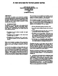
Figure 1: Lazy multiplication by the naive algorithm
Figure 2: Lazy multiplication by Karatsuba's algorithm
known. Although f1 g1 does not contribute to the coef cient (fg)1 = f0 g1 + f1 g0 , its premature computation accelerates the computation of (fg)2 at the next stage. The lazy computation process of fg by Karatsuba's algorithm is represented schematically in gure 2. Each box corresponds to the contribution of fi gj to the sum P i +j (fg)i+j = k=0 fk gi+j k. The number si;j in the box corresponds to the round when the contribution of fi gj is computed, i.e. when (fg)s is output. For comparison, we have represented the computation process of fg by the algorithm (i.e. (fg)n is computed by (fg)n = Pn naive k=0 fk gn k ) in gure 1. Let us now show how the idea of premature computations can be exploited even more. Observe rst, that if the rst 2p+1 coe�cients of f and g are known, then the multiplication
new array elements is zero. Now we undertake the following action to compute A[n] (where we assume that f0 ; � � � ; fn; g0; � � � ; gn are known and A[0]; � � � ; A[n 1] have already been computed):
i;j
+1
) �2 ;2 = (f2 z + � � � + f2 +1 1 z +1 1 2 2 ) (g2 z + � � � + g2 +1 1 z can be performed prematurely by any fast static multiplication algorithm. More generally, if the rst n = (k + 1)2p coe�cients of f and g are known, with k 2 f2; 3; � � �g and p > 1, then the multiplications p
p
p
2p
2p
p
p
1
p
p
p
�2 ;k2 = (f2 z 2 + � � � + f2 +1 1z 2 +1 1) (gk2 z k2 + � � � + g(k+1)2 1 z (k+1)2 and �k2 ;2 = (fk2 z k2 + � � � + f(k+1)2 1z (k+1)2 (g2 z 2 + � � � + g2 +1 1 z 2 +1 1 ) can be performed prematurely. p
p
p
p
p
p
p
p
p
p
p
p
p
1
)
p
1
)
p
p
p
p
p
p
Fast lazy multiplication. Let us now detail how the above observations can be transformed into a lazy multiplication algorithm. The coe�cients (fg)0 ; (fg)1 ; � � � of the result are stored in an array A, which is resized automatically, each time when necessary; the default value of
Step 1. [Border] If n = 0, then set A[0] := f g . 0 0
Otherwise, set A[n] := A[n] + f0 gn + fn g0. Step 2. [Diagonal] If n = 2p+1 for some p > 0, then compute �2 ;2 and set A[i] := A[i] + �2 ;2 ;i for all 2p+1 6 i 6 2p+2 2. Step 3. [Main] For each k > 2 and p > 0 such that n = (k + 1)2p , do the following: Compute �2 ;k2 and set A[i] := A[i] + �2 ;k2 ;i for all (k + 1)2p 6 i 6 (k + 3)2p 2. Compute �k2 ;2 and set A[i] := A[i] + �k2 ;2 ;i for all (k + 1)2p 6 i 6 (k + 3)2p 2. p
p
p
p
p
p
p
p
p
p
p
p
Correctness proof. The computation process is schematically represented in gure 3. From this gure, it is easily seen that the contribution of each fi gj to (fg)i+j is computed exactly once and before the coe�cient (fg)i+j is output. This proves the correctness of our algorithm. Complexity analysis. Let us now estimate the asymptotic complexity T (n) of the computation of (fg)n by our algorithm. If n = 2p , then in order to compute the contribution of (f0 + � � � + fn 1z n 1)(g0 + � � � + gn 1z n 1); (2) to fg, we need (2n 1) + (2n 3) constant multiplications, n 3 multiplications of polynomials of degree one, n=2 3 multiplications of polynomials of degree three, etc. (by looking at gure 3). Let M (d) = d� log d log log d be a complexity bound for the multiplication of two polynomials of degree d 1, as in the introduction. In view of what precedes, the time T~(n) needed to compute the contribution
.. . g7 g6 g5 g4 g3 g2 g1 g0
8 7 6 5 4 3 2 1 0 � f0
.. . 8 7 6 5 4 3 2 1 f1
.. .
.. .
8 6
���
8
4 6 3 4 5 6 2 3 4 5 f2 f3 f4 f5
8 ��� 7 8 ��� 6 7 8 f6 f7 � � �
Figure 3: Fast lazy multiplication of (2) to fg is bounded by pX1 2 2nk M (2k ) + O(n) = O(M (n) log n): (3) k=0 For general n > 2, this yields T (n) = O(M (n) log n), since T~(2blog2 nc) 6 T (n) 6 T~(2blog2 nc+1 ): The space needed for the computation of (fg)n is clearly bounded by O(n). This completes the proof of theorem 2.
Remark. Sometimes, we need a lazy multiplication algorithm for power series, which computes only the rst n coe�cients of the product (i.e. for the expansion of implicit functions). In this case, it is not hard to modify the above algorithm, so that no \unnecessary premature computations" are done, which anticipate the computations of (fg)n ; (fg)n+1 ; � � � . 4 Conclusion
Let us discuss some of the consequences of theorem 2. An important application of lazy multiplication is the resolution of algebraic di�erential equations X P f i0 � � � (f (r) )i = 0 (4) i0 ;��� ;i i0 ;��� ;ir
r
r
with power series coe�cients and suitable initial conditions. Although Brent and Kung have given an asymptotically better algorithm to solve such equations in [1], the constant involved in their asymptotic estimate O(n log n) of the time complexity depends badly on r, whereas the constant involved in our algorithm only depends on the size of (4) as an expression. Therefore, we expect our algorithm to be often faster for not all to large n. Similarly, both our algorithm and Brent and Kung's algorithm require O(n) memory space, but the constant factor involved in this bound is usually much smaller
for our algorithm. Here we notice that for many applications the available memory space is the main bottleneck. Another advantage of our algorithm is that it is easy to implement and that it can easily be applied to solve systems of ordinary di�erential equations as well. Our lazy multiplication algorithm can also be used to solve more general functional equations, such as 3 3 (5) s(z ) = 1 + z s(z ) +3 2s(z ) ; which occurs in the study of the number of stereoisomeres of alcohols of the form Cn H2n+1OH (see [4]). Then theorem 2 implies that the asymptotic complexity to compute the rst n coe�cients of s(z ) is O(n log2 n), which is much better than the previously best known bound O(n2). Many other di�erential di�erence equations arising in combinatorics and the analysis of algorithms are similar to (5) (see also [2]). This is in particular so for binary splitting algorithms, such as the algorithms presented in this paper themselves! Let us nally remark that for the fast expansion of power series which satisfy more complicated di�erential di�erence equations, it would be nice to extend the ideas of this paper in order to obtain lazy versions of Brent and Kung's fast algorithms for functional composition and inversion (see [1]). Acknowledgment. The author thanks the referees for their detailed comments, and for having pointed out some mistakes in the original version of this paper. References
[1] Brent, R., and Kung, H. Fast algorithms for manipulating formal power series. Journal of the Association for Computing Machinery 25, 4 (1978), 581{595. [2] Flajolet, P., and Sedgewick, R. An introduction to the analysis of algorithms. Addison Wesley, Reading, Massachusetts, 1996. [3] Knuth, D. The art of computer programming, vol. 2: seminumerical algorithms. Addison Wesley, Reading, Massachusetts, 1981. [4] Po�lya, G. Kombinatorische Anzahlbestimmungen fur Gruppen, Graphen und chemische Verbindungen. Acta Mathematica 68 (1937), 145{254. [5] Schonhage, A. Schnelle Multiplikation uber Korpern der Charakteristik 2. Acta Inform. 7 (1977), 395{398.