数理解析研究所講究録 1106 巻 1999 年 161-173
161
Lazy Narrowing Calculi: Strong Completeness, Eager Variable Elimination, Nondeterminism, Optimality Aart Middeldorp Institute of Information Sciences and Electronics University of Tsukuba, Tsukuba 305-8573, Japan ami@is. tsukuba.
http:
$//\mathrm{w}\mathrm{w}\mathrm{w}$
$\mathrm{a}\mathrm{c}$
. jp
. score. is. tsukuba.
$\mathrm{a}\mathrm{c}.\mathrm{j}\mathrm{p}/\sim \mathrm{a}\mathrm{m}\mathrm{i}$
Satoshi Okui Faculty of Engineering Mie University, Tsu 514-8507, Japan
[email protected] http: .inf .mie-u. $//\mathrm{w}\mathrm{w}\mathrm{w}.\mathrm{c}\mathrm{s}$
$0$
$\mathrm{a}\mathrm{c}.\mathrm{j}\mathrm{p}/\sim \mathrm{o}\mathrm{k}\mathrm{u}\mathrm{i}$
Abstract
Narrowing is an important method for solving unification problems in equational theories that are presented by confluent term rewriting systems. Because narrowing is a rather complicated operation, several authors studied calculi in which narrowing is replaced by more simple inference rules. In this paper we give an overview of the results that have been obtained by Middeldorp et al. $[19, 18]$ for the lazy narrowing calculus
1
$\mathrm{L}\mathrm{N}\mathrm{C}$
.
Introduction
Narrowing [13] is genera,1 method for solving unification problems in equational theories that are presented by confluent term rewrite systems (TRSs for short). Consider e.g. the TRS consisting of the following three rewrite rules, specifying subtraction on natural numbers:
$\mathcal{R}$
$0-y$
$arrow$
$0$
$x-0$
$arrow$
$x$
$\mathrm{s}(x)-\mathrm{s}(y)$
$arrow$
$x-y$
162 , i.e., we want to find a substituSuppose we want to solve the equation tion for the variables and such that both terms become equal in the equational theory generated by . The following rewrite sequence, where in each step the selected redex is is a solution: underlined, shows that the substitution $\mathrm{s}(\mathrm{s}(x-y))\approx \mathrm{s}(x)$
$x$
$y$
$\mathcal{R}$
$\theta=\{x\vdasharrow \mathrm{s}(\mathrm{O}), y\vdasharrow \mathrm{s}(\mathrm{O})\}$
$\mathrm{s}(\mathrm{s}(\mathrm{s}(0)-\mathrm{s}(0)))\approx \mathrm{s}(\mathrm{s}(0))$
$arrow \mathrm{s}(\mathrm{s}(\underline{0-0}))\approx \mathrm{s}(\mathrm{s}(0))$
$arrow \mathrm{s}(\mathrm{s}(0))\approx \mathrm{s}(\mathrm{s}(0))$
In term rewriting a subterm can be reduced only if it matches a left-hand side of a rewrite rule. In narrowing unification rather than matching is used, so variables in the term at hand may be instantiated before a rewrite step is performed. For instance, the equation for and cannot be reduced by rewriting but if we substitute can be reduced by applying for then the resulting equation . In order to guarantee a finitely branching the third rewrite rule to the subterm search space, variables are instantiated in a minimal way such that a rewrite step can be performed. Continuing the above example, a possible narrowing computation is $x$
$\mathrm{s}(x_{1})$
$\mathrm{s}(\mathrm{s}(x-y))\approx \mathrm{s}(x)$
$\mathrm{s}(y_{1})$
$\mathrm{s}(\mathrm{s}(\mathrm{s}(x_{1})-\mathrm{s}(y_{1})))\approx \mathrm{s}(\mathrm{s}(x_{1}))$
$y$
$\mathrm{s}(x_{1})-\mathrm{s}(y_{1})$
$\mathrm{s}(\mathrm{s}(x-y))\approx \mathrm{s}(x)$
$\sim+_{\theta_{1}}$
$\mathrm{s}(\mathrm{s}(\underline{x_{1}-y_{1}}))\approx \mathrm{s}(\mathrm{s}(x_{1}))$
$\mathrm{s}(\mathrm{s}(x_{1}))\approx \mathrm{s}(\mathrm{s}(x_{1}))$ $\sim*_{\theta_{2}}$
. Since the two sides of the final and with gives a solution to the initial equation equation are identical, the composition of and , as one easily verifies. The property that successful (i.e., ending in an equation whose sides are syntactically unifiable) narrowing derivations produce solutions is known as the soundness of narrowing. Narrowing is known to be complete for confluent TRSs with respect to normalized solutions. (A substitution is normalized if it substitutes for every confluent TRS , for every equation normal forms for the variables.) That $e=s\approx t$ , and for every normalized solution of , there exists a successful narrowing derivation starting from which produces a substitution that is, when restricted to the variables in , at least as general . The restriction to confluent TRSs is essential as shown with respect to the non-confluent TRS {a }: the by the equation empty substitution is a solution (as and are equal in the induced equational theory) but with respect to the one-rule narrowing is not applicable to . The equation shows the necessity of the normalization requirement: the non-normalized TRS is a solution of but narrowing is not applicable. substitution Narrowing is the underlying computation mechanism of many programming language that integrate the functional and logic programming paradigms (Hanus [7]). Since narrowing is a complicated operation, numerous calculi consisting of a small number of more elementary inference rules that simulate narrowing have been proposed, e.g. by Martelli al. $[16, 15]$ , H\"olldobler $[10, 11]$ , Snyder [20], Dershowitz et al. [3], Hanus $[8, 9]$ , Ida and Nakahara [14], and B\"utow et al. [2]. These calculi are highly nondeterministic: in general all choices of (1) $\theta_{2}=\{y_{1}rightarrow 0\}$
$\theta_{1}=\{x\vdash+\mathrm{s}(x_{1}), yrightarrow*\mathrm{s}(y_{1})\}$
$\theta_{2}$
$\theta_{1}$
$\mathrm{s}(\mathrm{s}(x-y))\approx \mathrm{s}(x)$
$\mathcal{R}$
$\mathrm{i}\mathrm{s}_{7}$
$\theta$
$e$
$\theta’$
$e$
$\theta$
$e$
$e=\mathrm{b}\approx \mathrm{c}$
$arrow \mathrm{b},$
$\mathrm{a}arrow \mathrm{c}$
$\mathrm{b}$
$\mathrm{c}$
$e=x\approx \mathrm{f}(x)$
$e$
$\{\mathrm{a}arrow \mathrm{f}(\mathrm{a})\}$
$\{x\vdasharrow \mathrm{a}\}$
$e$
$et$
163
the equation in the current goal, (2) the inference rule to be applied, and (3) the rewrite rule of the TRS (for certain inference rules) have to be considered in order to guarantee completeness. In this paper we investigate under what conditions which of these choices can be eliminated without affecting completeness. So the aim of our work is to reduce the huge search space by minimizing the nondeterminism while retaining completeness. We do this for the lazy nawowing calculus ( for short), which is the specialization to confluent TRSs and narrowing of the H\"olldobler’s calculus TRANS ([11]), which is defined for general equational systems and based on paramodulation. consists of the following five rules: $[0]$ outermost narrowing $\mathrm{L}\mathrm{N}\mathrm{C}$
$\mathrm{L}\mathrm{N}\mathrm{C}$
$\inf_{\backslash }\mathrm{e}\mathrm{r}\mathrm{e}\mathrm{n}\mathrm{c}\mathrm{e}$
$\frac{G’,f(s_{1},.\cdot.\cdot.,s_{n})\simeq t,G’’}{G’,s_{1}\approx l_{1},.,s_{n}\approx l_{n},r\approx t,G’’}$
$[\mathrm{i}]$
if there exists a fresh variant imitation
$f(l_{1}, \ldots, l_{n})arrow r$
of a rewrite rule in
$\mathcal{R}$
,
,
$\frac{G’,f(s_{1},\ldots,s_{n})\simeq x,G’’}{(G’,s_{1}\approx x_{1},\ldots,s_{n}\approx x_{n},G’)\theta}$
$[\mathrm{d}]$
if $\theta=\{x\vdash+f(x_{1}, \ldots , x_{n})\}$ with decomposition
$x_{1},$
$\ldots,$
$x_{n}$
fresh variables,
,
$, \frac{G’,f(s_{1},\ldots,s_{n}).\approx f(t_{1},\ldots,t_{n}),G’’}{G,s_{1}\approx t_{1},..,s_{n}\approx t_{n},G’’}$
$[\mathrm{v}]$
variable elimination
,
$\frac{G’,s\simeq x,G’’}{(G’,G’)\theta}$
if removal
and $\theta=\{x-*s\}$ , of trivial equations
$x\not\in \mathcal{V}\mathrm{a}\mathrm{r}(s)$
$[\mathrm{t}]$
$\frac{G’,x\approx x,G’’}{G’,G’},\cdot$
In the rules $[0],$ , and stands for or . Contrary to usual narrowing, the $[0]$ outermost narrowing rule generates new parameter-passing equations , besides the body equation . These parameter-passing equations must eventually be solved, but we do not require that they are solved right away. If and $G’$ are the upper and lower goal in the inference rule , we write . This is called an -step. The applied rewrite rule or substitution may be supplied as subscript, i.e., we will write things like and . A finite -derivation Inay be abbreviated to where . An -refutation is an LNCderivation ending in the empty goal . $[\mathrm{i}]$
$[\mathrm{v}],$
$s\simeq t$
$s\approx t$
$t\approx s$
$s_{1}\approx l_{1},$
$\ldots$
$s_{n}\approx l_{n}$
$r\approx t$
$G$
$[\alpha](\alpha\in\{0, \mathrm{i}, \mathrm{d}, \mathrm{v}, \mathrm{t}\})$
$G\Rightarrow_{[\alpha]}G’$
$\mathrm{L}\mathrm{N}\mathrm{C}$
$G\Rightarrow_{[\circ],larrow r}G’$
$G\Rightarrow_{[i],\theta}G’$
$\theta=\theta_{1}\cdots\theta_{n-1}$
$G_{1}\Rightarrow_{\theta}^{*}G_{n}$
$\square$
$\grave{G}_{1}\Rightarrow\theta_{1}\ldots\Rightarrow\theta_{n-1}G_{n}$
$\mathrm{L}\mathrm{N}\mathrm{C}$
$\mathrm{L}\mathrm{N}\mathrm{C}$
164 In the remainder of the paper we summarize the results obtained in $[18, 19]$ . In the next section we address the nondeterminism due to the choice of the equation in the inference rules. In Sections 3 and 4 we consider the nondeterminism due to the choice of the inference rule. We make some concluding remarks in Section 5. Due to lack of space, we omit several results and all proofs. The interested reader is referred to $[18, 19]$ for details.
2
Strong Completeness
Consider again the TRS -derivation: following
$\prime \mathcal{R}$
defined in the beginning of the previous section. We have the
$\mathrm{L}\mathrm{N}\mathrm{C}$
$\mathrm{s}(\mathrm{s}(x-y))\approx \mathrm{s}(x)$
$\Downarrow[\mathrm{d}]$
$\mathrm{s}(x-y)\approx x$
$\Downarrow[i]$
$\{xrightarrow \mathrm{s}(x_{1})\}$
$\mathrm{s}(x_{1})-y\approx x_{1}$
$\Downarrow[0]$
$\mathrm{s}(x_{1})\approx x_{2},$
$y\approx 0,$ $x_{2}\approx x_{1}$
$\Downarrow[\mathrm{v}]$
$y\approx 0,$
$x_{2}-0arrow x_{2}$
$\{x_{2}rightarrow \mathrm{s}(x_{1})\}$
$\mathrm{s}(x_{1})\approx x_{1}$
$\Downarrow[\mathrm{v}]$
$\{yrightarrow 0\}$
$\mathrm{s}(x_{1})\approx x_{1}$
$\Downarrow[\mathrm{i}]$
$\{x_{1}\vdasharrow \mathrm{s}(x_{3})\}$
$\mathrm{s}(x_{3})\approx x_{3}$
Since the only applicable inference rule at this point is , it is clear that this derivation will not produce any solution. To obtain a solution we have to use a different rewrite rule in the $[\mathrm{i}]$
$\Rightarrow 0$
-step: $\mathrm{s}(x_{1})-y\approx x_{1}$
$\mathrm{s}(x_{2})-\mathrm{s}(y_{2})arrow x_{2}-y_{2}$
$\Downarrow[0]$
$\mathrm{s}(x_{1})\approx \mathrm{s}(x_{2}),$
$y\approx \mathrm{s}(y_{2}),$
$x_{2}-y_{2}\approx x_{1}$
$\Downarrow[\mathrm{d}]$
$x_{1}\approx x_{2},$ $y\approx \mathrm{s}(y_{2}),$
$x_{2}-y_{2}\approx x_{1}$
$\Downarrow[\mathrm{v}]$
$y\approx \mathrm{s}(y_{2}),$
$\{x_{1}-\neq x_{2}\}$
$x_{2}-y_{2}\approx x_{2}$
$\Downarrow[\mathrm{v}]$
$\{y\mapsto+\mathrm{s}(y_{2})\}$
$x_{2}-y_{2}\approx x_{2}$
$\Downarrow[0]$
$0-x_{3}arrow 0$
$x_{2}\approx 0,$ $y_{2}\approx x_{3},0\approx x_{2}$
$\Downarrow[\mathrm{v}]$
$\{x_{2}rightarrow 0\}$
165
$y_{2}\approx x_{3},0\approx 0$
$\{y_{2}\mapsto+x_{3}\}$
$\Downarrow[\mathrm{v}]$
$0\approx 0$
$\Downarrow[\mathrm{d}]$
$\square$
In this refutation, which computes the solution , the leftmost equation in every goal is selected. We will later see that is always safe to select the leftmost equation. In other words, with respect to leftmost selection is complete (for confluent TRSs and normalized solutions). One may be tempted to think that the selection of equations in goals never matters, but this is not the case. Consider the TRS consisting of the three rewrite rules $\{x\vdasharrow \mathrm{s}(\mathrm{O}), y\vdash\Rightarrow \mathrm{s}(y_{3})\}$
$\mathrm{L}\mathrm{N}\mathrm{C}$
$\mathcal{R}$
$\mathrm{f}(x)$
$arrow$
$\mathrm{g}(\mathrm{h}(x), x)$
$\mathrm{g}(x, x)$
$arrow$
a
$\mathrm{b}$
$arrow$
$\mathrm{h}(\mathrm{b})$
and the equation . Confluence of can be proved by a routine induction argument on the structure of terms and some case analysis. The (normalized) empty substitution is a solution of because $e=\mathrm{f}(\mathrm{b})\approx \mathrm{a}$
$\epsilon$
$\mathcal{R}$
$e$
$\mathrm{f}(\mathrm{b})arrow \mathrm{g}(\mathrm{h}(\mathrm{b}), \mathrm{b})arrow \mathrm{g}(\mathrm{h}(\mathrm{b}), \mathrm{h}(\mathrm{b}))arrow \mathrm{a}$
There is essentially only one equation is selected: $\mathrm{f}(\mathrm{b})\approx \mathrm{a}$
$\mathrm{L}\mathrm{N}\mathrm{C}$
-derivation starting from
$\Rightarrow[0],\mathrm{f}(x)arrow \mathrm{g}(\mathrm{h}(x),x)$
$\Rightarrow[0],\mathrm{g}(x_{1},x_{1})arrow \mathrm{a}$
$\Rightarrow[\mathrm{d}]$
$\Rightarrow[\mathrm{v}],\{x_{1}rightarrow x\}$
$\Rightarrow[\mathrm{i}],\{x\mapsto \mathrm{h}(x_{2})\}$
$e$
in which always the rightmost
$\mathrm{b}\approx x,$ $\mathrm{g}(\mathrm{h}(x), x)\approx \mathrm{a}$
$\mathrm{b}\approx x,$
$\mathrm{h}(x)\approx x_{1},$
$\mathrm{b}\approx x,$
$\mathrm{h}(x)\approx x_{1},$ $x\approx x_{1}$
$\mathrm{b}\approx x,$
$\mathrm{h}(x)\approx x$
$x\approx x_{1},$
$\mathrm{a}\approx \mathrm{a}$
$\mathrm{b}\approx \mathrm{h}(x_{2}),$ $\mathrm{h}(x_{2})\approx x_{2}$
$\Rightarrow[i],\{x_{2}rightarrow \mathrm{h}(x_{3})\}$
This is clearly not a refutation. (The alternative binding in -step results in a variable renaming of the above -derivation.) Hence completeness of is not independent of selection funciions. In other words, lacks the so-called strong completeness property (contradicting H\"olldobler [11, Corollary 7.3.9]). In [19] it is shown that is strongly complete whenever basic narrowing is complete. Basic narrowing (Hullot [13]) is a restriction of narrowing with the property that narrowing steps are never applied to a subterm introduced by a previous narrowing substitution. Basic narrowing has a much smaller search space than narrowing. Hence additional requirements are needed to ensure $\{x\vdash\not\simeq x_{1}\}$
$\mathrm{t}\mathrm{h}\mathrm{e}\Rightarrow[\mathrm{v}]$
$\mathrm{L}\mathrm{N}\mathrm{C}$
$\mathrm{L}\mathrm{N}\mathrm{C}$
$\mathrm{L}\mathrm{N}\mathrm{C}$
$\mathrm{L}\mathrm{N}\mathrm{C}$
166
its completeness. Three such conditions are mentioned in the literature (Hullot [13], Middeldorp and Hamoen [17] : termination, right-linearity, and orthogonality (under the additional . condition stated below). Hence we obtain the following strong completeness results for $)$
$\mathrm{L}\mathrm{N}\mathrm{C}$
Theorem 2.1 Let
normalized solution $\theta’\leq\theta[\mathcal{V}\mathrm{a}\mathrm{r}(G)],$
$\mathcal{R}$
a selection function, and a goal. For every respecting such that there exists an -refuiation one of the following conditions is satisfied:
confluent
be a
of
$\theta$
1.
$\prime \mathcal{R}$
is terminating,
2.
$\mathcal{R}$
is
3.
$\mathcal{R}$
is orthogonal and
$G$
$S$
$G$
$provi,ded$
$right- linear_{f}$
$TRS,$
$G\Rightarrow_{\theta}^{*},$
$\mathrm{L}\mathrm{N}\mathrm{C}$
$S$
$\square$
or $G\theta$
has a normal form.
$\square$
The above counterexample against strong completeness does not refute the completeness can be solved by always selecting the leftmost equation: . The goal of $\mathrm{f}(\mathrm{b})\approx \mathrm{a}$
$\mathrm{L}\mathrm{N}\mathrm{C}$
$\mathrm{f}(\mathrm{b})\approx \mathrm{a}$
$\Rightarrow[0],\mathrm{f}(x)arrow \mathrm{g}(\mathrm{h}(x),x)$
$\mathrm{b}\approx x,$
$\mathrm{g}(\mathrm{h}(x), x)\approx \mathrm{a}$
$\mathrm{g}(\mathrm{h}(\mathrm{b}), \mathrm{b})\approx \mathrm{a}$ $\Rightarrow[\mathrm{v}],\{xrightarrow \mathrm{b}\}$
$\mathrm{h}(\mathrm{b})\approx x_{1},$
$\mathrm{b}\approx x_{1},$
$\mathrm{a}\approx \mathrm{a}$
$\Rightarrow[\circ],\mathrm{g}(x_{1},x_{1})arrow \mathrm{a}$
$\mathrm{b}\approx \mathrm{h}(\mathrm{b}),$
$\mathrm{a}\approx \mathrm{a}$
$\Rightarrow[\mathrm{v}],\{x_{1}rightarrow \mathrm{h}(\mathrm{b})\}$
$\mathrm{h}(\mathrm{b})\approx \mathrm{h}(\mathrm{b}),$
$\mathrm{a}\approx \mathrm{a}$
$\Rightarrow[0],\mathrm{b}arrow \mathrm{h}(\mathrm{b})$
$\mathrm{b}\approx \mathrm{b},$
$\mathrm{a}\approx \mathrm{a}$
$\Rightarrow[\mathrm{d}]$
$\mathrm{a}\approx \mathrm{a}$ $\Rightarrow[\mathrm{d}]$
$\square$ $\Rightarrow[\mathrm{d}]$
This is not a coincidence, because we have the following completeness theorem ([19]). Theorem 2.2 Let there exists an $G$
$\mathcal{R}$
$\mathrm{L}\mathrm{N}\mathrm{C}$
confluent -refutation be a
$TRS$
$G\Rightarrow_{\theta}^{*},$
$\square$
and a goal. For every normalized solution . respecting such that $G$
$S_{1\mathrm{e}\mathrm{f}\mathrm{t}}$
$\theta’\leq\theta[\mathcal{V}\mathrm{a}\mathrm{r}(G)]$
$\theta$
of $\square$
is the selection function that always selects the leftmost equation. So the Here due to the selection of the equation is avoided if we adopt the nondeterminism of leftmost equation, which we do from now on. Hence in the remainder of the paper we assume that the sequence of equations $G’$ to the left of the selected equation in the inference is empty. rules of $S_{1\mathrm{e}\mathrm{f}\mathrm{t}}$
$\mathrm{L}\mathrm{N}\mathrm{C}$
$\mathrm{L}\mathrm{N}\mathrm{C}$
167
$\mathrm{f}(\mathrm{b})\approx \mathrm{a}$
$\Downarrow[\circ]$
$\mathrm{b}\approx \mathrm{g}(x),$
$\mathrm{a}\approx \mathrm{a}$
$\Downarrow[0]$
$\mathrm{g}(\mathrm{b})\approx \mathrm{g}(x),$
$\mathrm{a}\approx \mathrm{a}$
$\Downarrow[\mathrm{d}]$
$\mathrm{b}\approx x,$
$\mathrm{a}\approx \mathrm{a}$
$\Rightarrow[0]$
$\mathrm{g}(\mathrm{b})\approx x,$
$\Rightarrow[\mathrm{i}]$
$\Downarrow[\mathrm{v}]$
$\mathrm{b}\approx x_{1},$
$\Downarrow[\mathrm{v}]$
$\mathrm{a}\approx \mathrm{a}$
$\Downarrow[\mathrm{d}]$
$\square$
Figure 1: The
$\mathrm{L}\mathrm{N}\mathrm{C}$
$\Rightarrow[0]$
$\mathrm{a}\approx \mathrm{a}$
$\Downarrow[\mathrm{d}]$
$\square$
$\mathrm{a}\approx \mathrm{a}$
$\Downarrow[\mathrm{v}]$
$\mathrm{a}\approx \mathrm{a}$
$\Downarrow[\mathrm{d}]$
3
$\mathrm{a}\approx \mathrm{a}$
$\square$
-refutations starting from
$\mathrm{f}(\mathrm{b})\approx \mathrm{a}$
.
Eager Variable Elimination
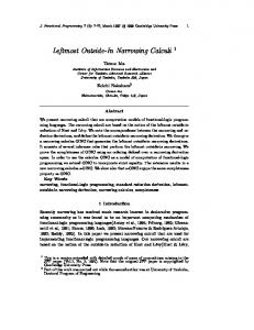
Next we turn out attention to the nondeterminism of due to the selection of the inference rule. The nondeterministic application of the various inference rules to selected (leftmost) equations causes to generate many redundant derivations. Consider for example the TRS consisting of the two rewrite rules $\mathrm{L}\mathrm{N}\mathrm{C}$
$\mathrm{L}\mathrm{N}\mathrm{C}$
$\mathrm{f}(\mathrm{g}(x))$
$\mathrm{b}$
$arrow$
$arrow$
a $\mathrm{g}(\mathrm{b})$
Figure 1 shows all -refutations starting from the goal . There are infinitely many such refutations, all computing the empty substitution. Hence for completeness it is suffices to compute only one of them. At several places in the literature it is mentioned that this type of redundancy can be greatly reduced by applying the variable elimination rule prior to other applicable inference rules, although to the best of our knowledge there is no supporting proof of this so-called eager variable elimination problem for the general case of confluent systems. In $[19, 18]$ it is shown that a restricted version of the eager variable elimination strategy is complete for left-linear confluent TRSs. The definition of the strategy relies on a notion of descendants for -derivations. The selected equation $f(s_{1}, \ldots, s_{n})\simeq t$ in the outermost narrowing rule $[0]$ has the body equation as only one-step descendant. In the imitation rule all equations are one-step descendants of the selected equation $f(s_{1}, \ldots, s_{n})\simeq x$ . The selected equation in the decomposition rule has all equations as one-step descendants. , the selected equations in and have no one-step descendants. One-step descendants of non-selected equations are defined as expected. Descendants are obtained from one-step descendants $\mathrm{L}\mathrm{N}\mathrm{C}$
$\mathrm{f}(\mathrm{b})\approx \mathrm{a}$
$[\mathrm{v}]$
$\mathrm{L}\mathrm{N}\mathrm{C}$
$r\approx t$
$s_{i}\theta\approx x_{i}(1\leq i\leq n)$
$[\mathrm{i}]$
$f(s_{1}, \ldots , s_{n})\approx f(t_{1}, \ldots, t_{n})$
$s_{1}\approx t_{1},$
$[\mathrm{d}]$
$[\mathrm{v}]$
$[\mathrm{t}]$
$\ldots,$
$s_{n}\approx t_{n}$
$\backslash \mathrm{F}\mathrm{i}\mathrm{n}\mathrm{a}\mathrm{l}\mathrm{l}\mathrm{y}$
168
-derivation descends by reflexivity and transitivity. Observe that every equation in an from either a parameter-passing equation or an equation in the initial goal. For example, descends from the parameter-passing equation in Figure 1 the equation -step. introduced in the -derivation is , is called solved. An An equation of the form $x\simeq t$ , with is applied to all selected solved equations that called eager if the variable elimination rule are descendants of a parameter-passing equation. $\mathrm{L}\mathrm{N}\mathrm{C}$
$\mathrm{b}\approx \mathrm{g}(x)$
$\mathrm{b}\approx x$
$\mathrm{f}\mathrm{i}\mathrm{r}\mathrm{s}\mathrm{t}\Rightarrow[\circ]$
$\mathrm{L}\mathrm{N}\mathrm{C}$
$x\not\in \mathcal{V}\mathrm{a}\mathrm{r}(t)$
$[\mathrm{v}]$
confluent $TRS$ -refutation
be a lefl-linear Theorem 3.1 Let solution of there exists an eager $\mathcal{R}$
$\theta$
4
$G$
and
$G\Rightarrow_{\theta}^{*},$
$\mathrm{L}\mathrm{N}\mathrm{C}$
$G$
a goal. For every normalized
$such$ that
$\theta’\leq\theta[\mathcal{V}\mathrm{a}\mathrm{r}(G)]$
.
Other Nondeterminism
In this section we address the remaining nondeterminism between the inference rules of First we consider descendants of parameter-passing equations. Consider the TRS :
$\mathrm{L}\mathrm{N}\mathrm{C}$
.
$\mathcal{R}$
$\mathrm{f}(\mathrm{a})$
$\mathrm{g}(\mathrm{f}(\mathrm{b}))$
$arrow$
$arrow$
$\mathrm{f}(\mathrm{b})$
$\mathrm{c}$
. Only the outermost narrowing rule $[0]$ is applicable to this goal, and the goal . To the parameter-passing equation resulting in the new goal we can either apply the decomposition rule followed by the variable elimination rule or and in the latter apply $[0]$ followed by . In the former case we obtain the solution . Since these solutions are incomparable (with respect to subsumption the solution modulo ), we cannot eliminate the nondeterminism between the outermost narrowing rule while retaining completeness. [o] and the decomposition rule The above situation cannot occur when we are dealing with left-linear constructor systems. A constructor system (CS for short) is a TRS with the property that the arguments of a rewrite rule are constructor terms. The of every left-hand side as folis partitioned into disjoint sets , and set of function symbols $F$ of a TRS such that if there is a rewrite rule lows: a function symbol belongs to $l=f(l_{1}, \ldots , l_{n})$ , otherwise are called constructors, those . Function symbols in defined symbols. A term built from constructors and variables is called a constructor in is not a CS because the defined symbol occurs in the term. Observe that the above . argument of the left-hand side In [18] it is shown that for left-linear confluent CSs all nondeterminism between the can be eliminated for descendants of parameter-passing equations. inferences rules of The proof is a consequence of the following lemma. $\mathrm{g}(\mathrm{f}(x))\approx \mathrm{c}$
$\mathrm{f}(x)\approx \mathrm{f}(\mathrm{b}),$
$\mathrm{f}(x)\approx \mathrm{f}(\mathrm{b})$
$\mathrm{c}\approx \mathrm{c}$
$[\mathrm{v}]$
$[\mathrm{d}]$
$\{x-t\mathrm{b}\}$
$[\mathrm{v}]$
$\{x\}arrow \mathrm{a}\}$
$\mathcal{R}$
$[\mathrm{d}]$
$l_{1},$
$f(l_{1}, \ldots , l_{n})$
$l_{n}$
$\ldots,$
$F_{D}$
$\mathcal{R}$
$f$
$larrow r\in \mathcal{R}$
$\mathcal{F}_{\mathcal{D}}$
$f\in \mathcal{F}_{C}$
$F_{C}$
$\mathcal{F}_{C}$
$F_{D}$
$\mathcal{R}$
$\mathrm{g}(\mathrm{f}(\mathrm{b}))$
$\mathrm{L}\mathrm{N}\mathrm{C}$
$\mathrm{f}$
169
Table 1: Selection of inference rule for descendant
root
$s\approx t$
of parameter-passing equation.
$(s)\backslash ^{\mathrm{r}\mathrm{o}\mathrm{o}\mathrm{t}(t)}$
$\mathcal{V} F_{C} F_{D}$
$\mathcal{V}$
$[\mathrm{v}] [\mathrm{v}] \cross$
$[\mathrm{v}] [\mathrm{d}] \cross$ $\mathcal{F}_{D}F_{C}$
$[\mathrm{v}] [0] \cross$
Lemma 4.1 Let be a lefl-linear $CS$ and an equation descends from a parameter-passing equation then is a constructor term. $\mathcal{R}$
$G\Rightarrow^{*}G’,$ $s\approx t,$
$G^{n}$
$\mathrm{L}\mathrm{N}\mathrm{C}$
-derivation. If the
$s\approx t$
$\mathcal{V}\mathrm{a}\mathrm{r}(G’, s)\cap \mathcal{V}\mathrm{a}\mathrm{r}(t)=\emptyset$
and
$t$
$\square$
The first part of Lemma 4.1 implies in particular that for every descendant of a parameter-passing equation, and have no variables in common. Hence we can forget about the occur-check in the variable elimination rule when dealing with such equations. The second part of the lemma implies that the outermost narrowing rule is only applicable to the left-hand side of descendants of parameter-passing equations. Moreover, if can be applied, then the decomposition rule is not applicable. Combining these observations with Theorem 3.1 yields complete determinism in the choice of inference rule for descendants of parameter-passing equations, provided of course we are dealing with left-linear confluent . Table 4 shows how the inference rule is completely determined by the root symbols of both sides of the selected descendant of a parameter-passing equation. The case root is impossible according to the second part of Lemma 4.1. Observe that the imitation rule is never applied to descendants of parameter-passing equations. This is because if is applicable then, according to the first part of Lemma 4.1, so is the variable elimination rule and by Theorem 3.1 the latter is given precedence. Next we turn our attention to descendants of equations in the initial goal. The following example shows that the restriction to left-linear confluent CSs is insufficient to remove all non-determinism in the choice of inference rule for descendants of initial equations. Consider the (left-linear ) CS $s\approx t$
$s$
$t$
$[\mathrm{v}]$
$[0]$
$[0]$
$[\mathrm{d}]$
$\mathrm{C}\mathrm{S}\mathrm{s}$
$s\approx t$
$(t)\in \mathcal{F}_{D}$
$[\mathrm{i}]$
$[\mathrm{i}]$
$[\mathrm{v}]$
$\mathrm{c}\mathrm{o}\mathrm{n}\mathrm{f}\mathrm{l}_{11}\mathrm{e}\mathrm{n}\mathrm{t}$
$\mathrm{f}(\mathrm{a})$
$arrow \mathrm{f}(\mathrm{b})$
and the goal . This goal has the two incomparable solutions and . The first solution can only be obtained if we apply the outermost narrowing rule $[0]$ . The second solution requires an application of the decomposition rule . There is also non-determinism in the outermost narrowing rule itself. Consider for example the CS $\mathrm{f}(x)\approx \mathrm{f}(\mathrm{b})$
$\{x\vdasharrow \mathrm{a}\}$
$\{x-+\mathrm{b}\}$
$[\mathrm{d}]$
$[0]$
$\mathrm{f}(\mathrm{a})$
$\mathrm{g}(\mathrm{b})$
and the goal
$\mathrm{f}(x)\approx \mathrm{g}(x)$
. The solution
$arrow$
$\mathrm{g}(\mathrm{a})$
$arrow$
$\mathrm{f}(\mathrm{b})$
$\{xrightarrow \mathrm{a}\}$
can only be obtained if we apply the
170
Table 2: Selection of inference rule for descendant root
$(s)\backslash ^{\mathrm{r}\mathrm{o}\mathrm{o}\mathrm{t}(t)}$
$\mathcal{V} F_{C} F_{D}$
$[\mathrm{v}]/[\mathrm{i}]^{b} [\mathrm{d}] [0]$
$F_{C}$
$[0] [0] [0]^{c}$
$F_{D}$
$b[\mathrm{v}]$
$c[0]$
of initial equation.
$[\mathrm{v}]/[\mathrm{t}] [\mathrm{v}]/[\mathrm{i}]^{a} [0]$
$\mathcal{V}$
$a[\mathrm{v}]$
$s\approx t$
is applied if and only if is applied if and only if is applied to the left-hand side
$t\in \mathcal{T}(F_{C}, \mathcal{V})$
$s\in \mathcal{T}(F_{C}, \mathcal{V})$
$s$
.
and and
$s\not\in \mathcal{V}\mathrm{a}\mathrm{r}(t)$
$t\not\in \mathcal{V}\mathrm{a}\mathrm{r}(s)$
.
.
, but in order to obtain the to the left-hand side of outermost narrowing rule to its right-hand side. it is essential that we apply incomparable solution In functional logic programming it is customary to consider two expressions to be equal if and only if they reduce to the same ground constructor normal form. This so-called strict as strict equality is adopted to model non-termination correctly $[4, 1]$ . If we interpret nor equality then the non-determinism in the above examples disappears: neither . A substitution and are (strict) solutions of the goals there exists a in if for every equation is said to be a strict solution of a goal . and constructor term such that Note that we do not require that the constructor term in the above definition is ground. Also note that a strict solution may substitute non-constructor terms for variables. In [18] it is shown that for confluent TRSs all nondeterminism between the inference rules of can be eliminated for descendants of initial equations with strict semantics. We would like to stress that the restriction to left-linear CSs is not needed here. Table 2 shows how the . It is interesting to note inference rule depends on the selected strictly solved equation that the resulting strategy is almost the opposite of eager variable elimination: conflicts are always and the outermost narrowing rule between the variable elimination rule resolved by giving preference to the latter and often the imitation rule $[i]$ is selected even if is applicable. $[0]$
$\mathrm{f}(x)\approx \mathrm{g}(x)$
$[0]$
$\{xrightarrow \mathrm{b}\}$
$\approx$
$\{xarrow+ \mathrm{a}\}$
$s\approx t$
$G$
$G$
$t\thetaarrow^{*}u$
$s\thetaarrow^{*}u$
$u$
$\theta$
$\mathrm{f}(x)\approx \mathrm{g}(x)$
$\mathrm{f}(x)\approx \mathrm{f}(\mathrm{b})$
$\{xrightarrow \mathrm{b}\}$
$u$
$\mathrm{L}\mathrm{N}\mathrm{C}$
$s\approx t$
$[0]$
$[\mathrm{v}]$
$[\mathrm{v}]$
5
Concluding Remarks
The results of the preceding two section can be directly incorporated into the inference for short, . This gives rise to the deterministic lazy narrowing calculus, rules of there is no nondeterminism between the whose inference rules can be found in [18]. In inference rules. In other words, at most one inference rule is applicable to every goal. $\mathrm{L}\mathrm{N}\mathrm{C}$
$\mathrm{L}\mathrm{N}\mathrm{C}_{\mathrm{d}}$
$\mathrm{L}\mathrm{N}\mathrm{C}_{\mathrm{d}}$
Theorem 5.1 Let be a lefl-linear confluent $CS$ and a goal. For every sfrict normalized , –such that . solution of there exists an -refutation $G$
$\prime \mathcal{R}$
$\theta$
$G$
$\mathrm{L}\mathrm{N}\mathrm{C}_{\mathrm{d}}$
$G\Rightarrow_{\theta}^{*}$
$\theta’\leq\theta[\mathcal{V}\mathrm{a}\mathrm{r}(G)]$
$\square$
171
In [18] it is further shown that substitutions computed by different derivations are incomparable, provided we are dealing with orthogonal . Hence for this subclass of TRSs solutions to goals are computed only once by . A similar result has been obtained for needed narrowing. Antoy et al. [1] define and prove the completeness of needed narrowing for inductively sequential TRSs. They present two optimality results for needed narrowing. First of all, only incomparable solutions are computed by needed narrowing. Since the class of inductively sequential TRSs coincides with the class of strongly sequential ([12]) orthogonal , our result shows that strong sequentiality is not essential for obtaining the incomparability of computed solutions. The second optimality result presented in [1] states that needed narrowing derivations have minimal length. This result has no counterpart in . We refer to [18] for a more thorough discussion of related work. We conclude this paper by mentioning that some of the results presented above have been extended to the more complicated setting of conditional term rewriting, see [5] and [6] for details. $\mathrm{L}\mathrm{N}\mathrm{C}_{\mathrm{d}}$
$\mathrm{C}\mathrm{S}\mathrm{s}$
$\mathrm{L}\mathrm{N}\mathrm{C}_{\mathrm{d}}$
$\mathrm{C}\mathrm{S}\mathrm{s}$
$\mathrm{L}\mathrm{N}\mathrm{C}_{\mathrm{d}}$
References [1] S. Antoy, R. Echahed, and M. Hanus. A needed narrowing strategy. In Proceedings of the 21st ACM Symposium on Principles of Programming Languages, pages 268-279,
1994. [2] B. B\"utow, R. Giegerich, E. Ohlebusch, and S. Thesing. Semantic matching for left-linear convergent rewrite systems. Journal of Functional and Logic Programming, 1999. To
appear.
[3] N. Dershowitz, S. Mitra, and G. Sivakumar. Decidable matching for convergent systems. In Proceedings of the 11th International Conference on Automated Deduction, volume 607 of LNAI, pages 589-602, 1992.
[4] E. Giovannetti, G. Levi, C. Moiso, and C. Palamidessi. Kernel-leaf: A logic plus functional language. Journal of Computer and System Sciences, $42(2):139-185$ , 1991. [5] M. Hamada and A. Middeldorp. Strong completeness of a lazy conditional narrowing calculus. In Proceedings of the 2nd Fuji International Workshop on Func tional and Logic Programming, pages 14-32. World Scientific, 1997.
[6] M. Hamada, A. Middeldorp, and T. Suzuki. Completeness results for a lazy conditional narrowing culus. In Combinatorics, Computaiion : Proceedings of 2nd Discrete Mathematics and Theoretical Computer Scie. onference and the 5th Australasian Theory Symposium, pages 217-231. Springer-Verlag Singapore, 1999. $\mathrm{c}\mathrm{a}\dot{\mathrm{l}}$
$\sim\backslash and\dot{L}_{\backslash }ogic$
$nce\grave{C}$
172
[7] M. Hanus. The integration of functions into logic programming: From theory to practice. Journal of Logic Programming, 19&20:583-628, 1994. [8] M. Hanus. Lazy unification with simplification. In Proceedings of the 5th European Symposium on Programming, volume 788 of LNCS, pages 272-286, 1994. [9] M. Hanus. Lazy narrowing with simplification. Computer Languages, $23(2-4):61-85$ ,
1997. [10] S. H\"olldobler. A unification algorithm for confluent theories. In Proceedings of the 14 th International Colloquium on Automata, Languages and Frogramming, volume 267 of LNCS, pages 31-41, 1987. [11] S. H\"olldobler. Foundations Springer Verlag, 1989.
of Equational
Logic Programming, volume 353 of LNAI.
[12] G. Huet and J.-J. L\’evy. Computations in orthogonal rewriting systems, I and II. In J.-L. Lassez and G. Plotkin, editors, Computational $Logic_{f}$ Essays in Honor of Alan Robinson, pages 396-443. The MIT Press, 1991. [13] J.-M. Hullot. Canonical forms and unification. In Proceedings of the 5th Automated Deduction, volume 87 of LNCS, pages 318-334, 1980.
Conference on
[14] T. Ida and K. Nakahara. Leftmost outside-in narrowing calculi. Journal Programming, $7(2):129-161$ , 1997.
of Functional
. Rossi. Lazy unification algorithms for canonical rewrite [15] A. Martelli, C. Moiso, and systems. In H. Ait-Kaci and M. Nivat, editors, Resolution of Equations in Algebraic Structures, Vol. II, Rewriting Techniques, pages 245-274. Academic Press, 1989. $\mathrm{G}.\mathrm{F}$
. Rossi, and C. Moiso. An algorithm for unification in equational [16] A. Martelli, theories. In Proceedings of the 1986 Symposium on Logic Programming, pages 180-186, $\mathrm{G}.\mathrm{F}$
1986. [17] A. Middeldorp and E. Hamoen. Completeness results for basic narrowing. Applicable Algebra in $Engineering_{f}$ Communication and Computing, 5:213-253, 1994. [18] A. Middeldorp and S. Okui. A deterministic lazy narrowing calculus. Journal bolic Computation, $25(6):733-757$ , 1998.
of Sym-
[19] A. Middeldorp, S. Okui, and T. Ida. Lazy narrowing: Strong completeness and eager variable elimination. Theoretical Computer Science, $167(1,2):95-130$ , 1996.
[20] W. Snyder. A
Proof Theory for General Unification. Birkh\"auser, 1991.
173
Solutions Week 2 2. No, the $\mathrm{f}(\mathrm{a}),$
not irreflexive. Consider for instance the infinite sequence . Since is a proper subterm of for all $i\geq 1$ , we have
$\mathrm{r}\mathrm{e}\mathrm{l}\mathrm{a}\mathrm{t}\mathrm{i}\mathrm{o}\mathrm{n}\subset \mathrm{i}\mathrm{s}$
$\mathrm{f}(\mathrm{f}(\mathrm{a})),$
$\ldots$
definition.
$t_{i}$
$t_{i+1}$
, by
$\mathrm{t}=\mathrm{a}$
$\mathrm{t}\subset \mathrm{t}$
3. Consider a signature $F$ consisting of a constant , a unary function symbol , and an -ary function symbol . We code natural numbers as terms in via the following mapping : $0$
$n$
$\mathrm{s}$
$\mathrm{c}$
$\mathcal{T}(\{0, \mathrm{s}\})$
$\phi$
$0$
$\phi(n)=\{$ $\mathrm{s}(\phi(n-1))$
if $n=0$ , if $n>0$ .
This mapping is extended to -tuples of natural numbers by defining $n$
$\phi((x_{1}, \ldots,x_{n}))$
$=$
$\mathrm{c}(\phi(x_{1}), \ldots, \phi(x_{n}))$
.
Now consider an infinite sequence of -tuples of natural numbers. By construction is an infinite sequence of terms in . According to Kruskal’s bee Theorem there exist $i