IEEE TRANSACTIONS ON COMMUNICATIONS, VOL. 58, NO. 2, FEBRUARY 2010
511
LDPC Code Design for Asynchronous Slepian-Wolf Coding Zhibin Sun, Chao Tian, Member, IEEE, Jun Chen, Member, IEEE, and Kon Max Wong, Fellow, IEEE
Abstract—We consider asynchronous Slepian-Wolf coding where the two encoders may not have completely accurate timing information to synchronize their individual block code boundaries, and propose LDPC code design in this scenario. A new information-theoretic coding scheme based on source splitting is provided, which can achieve the entire asynchronous Slepian-Wolf rate region. Unlike existing methods based on source splitting, the proposed scheme does not require common randomness at the encoder and the decoder, or the construction of super-letter from several individual symbols. We then design LDPC codes based on this new scheme, by applying the recently discovered source-channel code correspondence. Experimental results validate the effectiveness of the proposed method. Index Terms—Belief propagation, low density parity check codes, Slepian-Wolf coding, source splitting.
R2 H (Y ) achievable
H(Y | X)
H(X | Y)
I. I NTRODUCTION
I
N the seminal work [1], Slepian and Wolf showed that it is possible to compress two dependent sources in a distributed manner, at rates no larger than those needed when they are compressed jointly. More precisely, when two discrete memoryless sources 𝑋 and 𝑌 , jointly distributed as 𝑄𝑋𝑌 in the alphabets 𝒳 and 𝒴, are separately compressed using block codes of length-𝑛 at rates 𝑅1 and 𝑅2 , respectively, both sources can be reconstructed with asymptotically diminishing error probability at a central decoder, using any rates (𝑅1 , 𝑅2 ) such that 𝑅1 > 𝐻(𝑋∣𝑌 ), 𝑅2 > 𝐻(𝑌 ∣𝑋), 𝑅1 + 𝑅2 > 𝐻(𝑋, 𝑌 ). (1) This rate region is illustrated in Fig. 1. This result has been generalized in various ways [2]– [5], one of which is the asynchronous Slepian-Wolf (A-SW) coding scenario considered by Willems [4]. This consideration is practically important, because although we can assume perfect synchronization in the simplistic Slepian-Wolf setting such that the length-𝑛 block codes can be applied on each Paper approved by Z. Xiong, the Editor for Distributed Coding and Processing of the IEEE Communications Society. Manuscript received January 23, 2009; revised May 12, 2009. Z. Sun was with the Department of Electrical and Computer Engineering, McMaster University, Hamilton, ON, Canada. He is now with Hydro One Networks Inc., Toronto, ON, Canada (e-mail:
[email protected]). C. Tian is with AT&T Labs–Research, Florham Park, NJ, USA (e-mail:
[email protected]). J. Chen and K. M. Wong are with the Department of Electrical and Computer Engineering, McMaster University, Hamilton, ON, Canada (e-mail:
[email protected],
[email protected]). The material in this paper was presented in part at IEEE International Symposium on Information Theory, Seoul, Korea, June 2009. Digital Object Identifier 10.1109/TCOMM.2010.02.090034
Fig. 1.
H(X )
R1
The achievable rate region for Slepian-Wolf coding.
corresponding block pair, in practice the two encoders may not have such a perfectly accurate global clock to synchronize their block code boundaries. It was shown in [4] that even in this case, the rate region result (1) still holds, as long as the decoder is aware of this asynchronism. Thus, the restriction on the synchronization is in fact unnecessary and can be effectively removed, when the system is properly designed. In this work, we consider the code design in the A-SW setting. Formally, the encoders are associated with an integer delay pair (𝑑𝑥 , 𝑑𝑦 ), each in the range of 0 to 𝑛 − 1. The values of 𝑑𝑥 and 𝑑𝑦 are unknown to the encoders but known to the decoder. Thus the 𝑞-th block of the source 𝑋 consists of {𝑋(𝑡)}𝑡=𝑞𝑛+1+𝑑𝑥 ,...,(𝑞+1)𝑛+𝑑𝑥 and the 𝑞-th block of the source 𝑌 consists of {𝑌 (𝑡)}𝑡=𝑞𝑛+1+𝑑𝑦 ,...,(𝑞+1)𝑛+𝑑𝑦 . It is easy to see that for the two corner points of the achievable rate region, this problem is not very different from that in the synchronous case. Thus our focus is on the general rate pairs, i.e., rate pairs on the dominant face of the rate region. Previous works on the synchronous Slepian-Wolf (S-SW) code design mostly focus on the corner points of the rate region [7]–[10], with only a few exceptions [11][12]. The code design at the corner points is reasonably well understood, particularly with the recent development [13], where it was shown that when encoding 𝑌 𝑛 with side information 𝑋 𝑛 at the decoder, the error probability of any single linear coset code is exactly the decoding error probability of the same channel code on a corresponding channel under optimal decoding or belief propagation decoding. Thus the linear Slepian-Wolf
c 2010 IEEE 0090-6778/10$25.00 ⃝
512
code design problem at a corner point can be conveniently converted into the code design problem for a specific channel. Though this connection was mentioned in earlier works [14], [15], it was made precise in [13] for general (non-symmetric non-binary) sources. The code design for the S-SW problem cannot be applied directly to the asynchronous case. One may wonder if the information-theoretic coding scheme given in [4] can be used for such a purpose, however, it unfortunately requires optimization of the auxiliary random variable and complex joint typicality encoding usually seen in quantization modules, thus not convenient for practical code design. The usual timesharing approach to achieve general rate pairs in S-SW coding also does not apply in the asynchronous setting. In [16], an information-theoretic scheme based on source splitting was given to overcome this difficulty due to asynchronism, by introducing common randomness at one encoder and the decoder. However, common randomness is not desirable in practical systems and should be avoided if possible. It is clear that a new coding approach is needed for the A-SW code design, and since Slepian-Wolf coding is well understood for the corner points of the rate region, it is also desirable to utilize these existing results. Indeed, in this work we first present an information-theoretic scheme based on source splitting, which does not require common randomness (or the construction of a threshold function which operates on multiple source symbols as a super-letter [12]). Then based on this coding scheme, we utilize the source-channel correspondence result in [13] to design good LDPC codes. Experimental results confirm the effectiveness of the proposed design. Moreover, the proposed method does not significantly increase either system design or system implementation complexity compared to those of synchronized systems, and the performance is also comparable to state of the art design for synchronized systems in the literature. It should be clarified at this point that the asynchronism here only refers to the mismatch in the block code boundaries of the two encoders, but not the timing mismatch in the sampling process. When sampling a continuous process, such timing inaccuracy may incur uncertainty in the probability distribution 𝑃𝑋𝑌 , and this problem is usually considered in the framework of universal Slepian-Wolf compression [5][6], thus is beyond the scope of this work. II. A N EW S OURCE S PLITTING S CHEME FOR A-SW C ODING In this section, we first briefly explain the difficulty of using time-sharing in the asynchronous setting and then review how source splitting together with common randomness can be used to overcome this difficulty, as proposed in [16]. Then a new information-theoretic scheme based on source splitting is proposed, which does not require common randomness. An overview of the proposed LDPC code design in the context of this new scheme will be subsequently discussed. A. Time-sharing and Source Splitting With Common Randomness It is easy to see that a simple time-sharing can be used to achieve any general rate pair in the achievable rate region
IEEE TRANSACTIONS ON COMMUNICATIONS, VOL. 58, NO. 2, FEBRUARY 2010
…… X:
n samples encoded n samples encoded n samples encoded at rate H(X) at rate H(X|Y) at rate H(X)
…… ……
…… dx=½ n
Y:
……
(2k)-th block
…… n samples encoded at rate H(Y|X)
Fig. 2.
(2k+1)-th block
(2k+2)-th block
n samples encoded n samples encoded at rate H(Y) at rate H(Y|X)
…… ……
The difficulty of time-sharing in the asynchronous setting.
for the S-SW problem. Essentially we only need to use the following two kinds of coding alternately: 1) first encode 𝑋 directly, then encode 𝑌 with 𝑋 as decoder side information, and 2) first encode 𝑌 directly, then encode 𝑋 with 𝑌 as decoder side information. When the first kind of code is used with a proportion 𝑝, and the second is used with proportion 1 − 𝑝, it is clear that the following rate pair is achieved. 𝑅1 = 𝑝𝐻(𝑋) + (1 − 𝑝)𝐻(𝑋∣𝑌 ) 𝑅2 = 𝑝𝐻(𝑌 ∣𝑋) + (1 − 𝑝)𝐻(𝑌 ).
(2)
An example makes clear the difficulty of using this approach in the asynchronous setting. Let us assume 𝑝 = 0.5 and the two kinds of codes used in timesharing both are of length-𝑛. Thus in the synchronous setting, the first kind of code is used in the even block, i.e., the (2𝑚)-th block, and the second kind of code is used in the odd block, i.e., the (2𝑚 + 1)-th block. Now consider the asynchronous setting, and let 𝑑𝑥 = 12 𝑛 and 𝑑𝑦 = 0, which are unknown to the encoders but known to the joint decoder. When the original time-sharing codes are used, it is clear that at the first half of the even blocks, source 𝑌 is encoded assuming 𝑋 at the decoder, yet the source 𝑋 is also encoded assuming 𝑌 at the decoder. This clearly results in decoder failure. Another way to see this is that in this portion, the sources are encoded with sum rate 𝐻(𝑌 ∣𝑋) + 𝐻(𝑋∣𝑌 ), which is less than 𝐻(𝑋, 𝑌 ), and thus it is impossible to ensure reliable communication; see Fig. 2 for an illustration. To overcome this difficulty, common randomness was introduced in [16] such that source splitting can be applied. Let {𝑇 (𝑡)}𝑡=1,...,∞ be a binary discrete memoryless process distributed in {0, 1} such that at each time instance, Pr[𝑇 (𝑡) = 1] = 𝑝; it is independent of the sources (𝑋, 𝑌 ). Let this process be available at both the encoder observing 𝑋 and the decoder. Without loss of generality, let us assume 𝒳 = {1, 2, . . . , ∣𝒳 ∣}. Now define two new sources 𝑍 = 𝑋 ⋅ 𝑇,
𝑊 = 𝑋 ⋅ (1 − 𝑇 ).
(3)
In other words, {𝑍(𝑡)}𝑡=1,...,∞ is {𝑋(𝑡)}𝑡=1,...,∞ with certain position assigned to zero, while {𝑊 (𝑡)}𝑡=1,...,∞ is {𝑋(𝑡)}𝑡=1,...,∞ with the complement positions assigned to zero. Thus the source 𝑋 is split into two sources 𝑍 and 𝑊 . Notice that by definition 𝑇 is a deterministic function of 𝑍, since 𝑇 is only zero when 𝑍 is zero. With these two new sources, the original problem is transformed into Slepian-Wolf coding of sources (𝑍, 𝑊 ) and 𝑌 . The encoding can now be performed in a sequential order as follows: 1) Encode the source 𝑍 conditioned on 𝑇 ;
SUN et al.: LDPC CODE DESIGN FOR ASYNCHRONOUS SLEPIAN-WOLF CODING
2. n samples encoded at rate (1-p)H(Y)+pH(Y|X)
……
2) Encode source 𝑌 assuming 𝑍 at the decoder; 3) Encode 𝑊 assuming (𝑍, 𝑌 ) at the decoder. The rates at the two encoders are
……
X: ……
i-th block
(i+1)-th block
(i+2)-th block
……
dx>0
(4)
……
Observe that 𝑅1 + 𝑅2 = 𝐻(𝑍∣𝑇 ) + 𝐻(𝑊 ∣𝑍, 𝑌 ) + 𝐻(𝑌 ∣𝑍) = 𝐻(𝑋, 𝑌 ∣𝑇 ) = 𝐻(𝑋, 𝑌 ).
……
Y: ……
𝑅1 = 𝐻(𝑍∣𝑇 ) + 𝐻(𝑊 ∣𝑍, 𝑌 ) 𝑅2 = 𝐻(𝑌 ∣𝑍) = 𝐻(𝑌 ∣𝑍, 𝑇 ).
513
……
1. k samples 3. (n-k) samples Encoded at Encoded at rate rate H(X) H(X|Y) (a)
……
(5)
The rate pair in (4) is on the dominant face of the achievable rate region. By varying 𝑝 from 0 to 1, all the rate pairs on the dominant face can be achieved, at least for the S-SW case. A moment of thought should convince the readers that by applying the above block codes consecutively, the coding scheme can also be used in the asynchronous case without any change. Although this scheme can indeed achieve all rate pairs in the A-SW setting, it requires common randomness at one encoder and the decoder, which is not desirable in practice because the common randomness essentially requires the system to be more flexible in order to handle a large number of the side information erasure patterns. This problem is exacerbated in practice since pseudo-randomness must be used to replace this common randomness, which introduces the possibility that certain pseudo-random erasure pattern blocks may incur large decoding error probability and it may occur periodically. Next we propose a new scheme which does not require the common randomness (or pseudo-randomness) and thus avoids this problem; this new method only requires the system to handle a few side information erasure patterns, and it can be understood as an efficient de-randomized version of the afore-given scheme using common randomness. B. A Source Splitting Scheme Without Common Randomness From the source splitting scheme with common randomness afore-given, we can make the following two observations: 1) In the second coding step, for each length-𝑛 block of source 𝑌 , there are approximately 𝑝⋅𝑛 source 𝑋 samples available at the decoder; furthermore, the exact positions of these 𝑋 samples are known at the decoder. 2) Though the random sequence 𝑇 (𝑡) can potentially split 𝑋(𝑡) at each time instance into two random variables 𝑍(𝑡) and 𝑊 (𝑡), the overall effect is in fact to split the length-𝑛 source 𝑋 sequence in the time domain, such that the first item above can be made true. Based on these two observations, we propose the following information-theoretic scheme, which does not require common randomness. Instead of the random sequence 𝑇 (𝑡), let us consider a deterministic one { 1 ⌊𝑡⌋𝑛 − 𝑑𝑥 = 1, . . . , 𝑘 (6) 𝑇 (𝑡) = 0 otherwise where ⌊⋅⌋𝑛 is modulo-𝑛 operation. In other words, the first 𝑘 positions in a block aligned with the length-𝑛 source 𝑋 block are assigned 1, while the remaining 𝑛 − 𝑘 positions are assigned 0. After we apply the first coding step in the original source splitting scheme, a partial 𝑋 sequence is available
2. n samples encoded at rate (1-p)H(Y)+pH(Y|X)
……
Y: ……
…… dy>0
X: ……
i-th block ……
(i+1)-th block
……
(i+2)-th block
1.k samples 3. (n-k) k samples encoded at samples encoded at rate H(X) encoded at rate H(X) rate H(X|Y)
……
(b)
Fig. 3.
Illustration of the new scheme without common randomness.
at the decoder. Such a choice of 𝑇 (𝑡) indeed approximately satisfies the first observation discussed above, regardless the exact value of 𝑑𝑥 ; see Fig. 3 for an illustration. At this point, the second coding step in the original source splitting scheme still cannot be directly applied, since now there is no explicit source 𝑍 to simplify the coding module. We can now focus on the second coding step of encoding source 𝑌 using a length-𝑛 block code, where 𝑘 out of 𝑛 of the corresponding 𝑋 source samples are available at the decoder, whose positions are unknown to the encoder, but known to the decoder. These 𝑘 positions of source 𝑋 samples can be from a single length-𝑛 source 𝑋 coding block, or two separate length-𝑛 source 𝑋 coding blocks, which are illustrated in Fig. 3(a) and Fig. 3(b), respectively. The following (random) coding scheme for the second step is the key difference between the one in [16] and the one proposed in this work. For convenience, let us denote the set of positions (indexed) within this length-𝑛 block for which source 𝑋 samples are available at the decoder as 𝒜, where 𝒜 ⊆ {1, 2, . . . , 𝑛}. Consequently the set of the remaining positions within this block is denoted as 𝒜𝑐 . ∙ ∙ ∙
Random binning: each of 𝑦 𝑛 sequence is uniformly and independently assigned to one of 2𝑛𝑅2 bin indices; Encoding: the encoder sends the bin index of the 𝑌 source sequence; Decoding: if the known length-𝑘 source 𝑋 sequence from 𝒜 is 𝛿1 -typical, we then find a length-𝑛 source 𝑌 sequence in the corresponding bin, such that the following two typicality conditions hold (i) the length𝑘 vector by collecting the 𝑌 samples at the positions corresponding to 𝒜 is jointly 𝛿1 -typical with the known length-𝑘 𝑋 sequence, and (ii) the length-(𝑛−𝑘) vector by collecting the 𝑌 samples at the positions corresponding to 𝒜𝑐 is 𝛿2 -typical by itself.
In the above procedure, we have used the (weak) typicality definition in [22] (p. 51 and pp. 384-385). It is easier to
514
IEEE TRANSACTIONS ON COMMUNICATIONS, VOL. 58, NO. 2, FEBRUARY 2010
bound the decoding error if we view a single length-𝑛 source 𝑌 sequence as the combination of a length-𝑘 and a length(𝑛 − 𝑘) sequence. When both 𝑘 and 𝑛 − 𝑘 are sufficiently large, it is clear that with high probability, the original source sequence 𝑦 𝑛 indeed satisfy the two typicality conditions with high probability; we shall denote the probability of such error event that a source sequence fails one of the two conditions as 𝑃𝑒′ . We only need to bound the probability that another 𝑌 sequence is decoded instead of the correct one. By the wellknown properties of the typical sequences (see [22] pp. 51-53 and pp. 385-387), we see there are less than 2𝑘(𝐻(𝑌 ∣𝑋)+2𝛿1 ) length-𝑘 source 𝑌 sequences that are jointly 𝛿1 -typical with the known 𝛿1 -typical length-𝑘 source 𝑋, and there are less than 2(𝑛−𝑘)(𝐻(𝑌 )+𝛿2 ) 𝛿2 -typical length-(𝑛 − 𝑘) source 𝑌 sequences. Thus the decoding error in this step is bounded by 𝑃𝑒 ≤ 𝑃𝑒′ + 2−𝑛𝑅2 2𝑘(𝐻(𝑌 ∣𝑋)+2𝛿1 ) 2(𝑛−𝑘)(𝐻(𝑌 )+𝛿2 ) + 𝛿1 𝑛−𝑘 𝑘 = 𝑃𝑒′ + 2−𝑛[𝑅2 − 𝑛 (𝐻(𝑌 ∣𝑋)+2𝛿1 )− 𝑛 (𝐻(𝑌 )+𝛿2 )] + 𝛿1 , (7) where the last term 𝛿1 accounts for the error event that the known 𝑋 sample sequence at the decoder is in fact not typical. Thus if we choose sufficiently small 𝛿1 and 𝛿2 , as long as 𝑘 𝑛−𝑘 𝐻(𝑌 ) + 𝐻(𝑌 ∣𝑋) 𝑛 𝑛 ≈ (1 − 𝑝)𝐻(𝑌 ) + 𝑝𝐻(𝑌 ∣𝑋),
𝑅2 >
the decoding error vanishes as 𝑛 → ∞. This solves the second step in the source splitting scheme without any common randomness. It should be noted that the scheme inherently requires both 𝑘 and 𝑛 − 𝑘 to be large. For the third coding step, the decoding may have to wait until the next 𝑌 block is decoded; see Fig. 3(a) for an illustration. Nevertheless, it is not difficult to see that the third coding step in the original source splitting scheme can be used without much change. Thus we only need 𝑛−𝑘 𝑘 𝐻(𝑋) + 𝐻(𝑋∣𝑌 ) 𝑛 𝑛 ≈ 𝑝𝐻(𝑋) + (1 − 𝑝)𝐻(𝑋∣𝑌 ).
𝑅1 >
(8)
For sufficiently large 𝑛, by adjusting 𝑘, all rate pair on the dominant face of the Slepian-Wolf rate region can be effectively approached. We have shown that for a fixed set 𝒜, there indeed exists a sequence of codes that can approach the Slepian-Wolf limit. However, one key requirement in the A-SW problem is that a single code has to guarantee small error probability for all the possible cyclic shifts of 𝒜 induced by the asynchronism. By refining the probability bound for decoding error given above, we can indeed show that such a sequence of codes exists. However instead of proving this more technical result here, in the appendix we provide a proof for an even stronger and relevant result that linear codes under the same source splitting paradigm can achieve the A-SW limit. This serves as a more rigorous proof, as well as the theoretical basis for designing the LDPC codes, which are indeed linear. The following two observations are now worth noting. Firstly, the position of 𝑇 (𝑡) being 1 does not need to be the first 𝑘 positions. In fact, any pattern can be used with
𝑘 positions assigned 1, as long as the pattern is repeated for all the blocks. More specifically, for 𝑘/𝑛 = 𝑘 ′ /𝑛′ where 𝑘 ′ and 𝑛′ are coprime of each other, we can choose 𝑇 (𝑡) to be a sequence alternating between 𝑘 ′ ones, and 𝑛′ − 𝑘 ′ zeros; this choice gives the smallest number of side information erasure patterns that need to be considered among all (𝑛, 𝑘) pairs of the same ratio. In the simulations given in Section IV, this kind of 𝑇 (𝑡) sequences will always be assumed. Secondly the proposed scheme has the advantage that decoding errors do not propagate across blocks, because a single encoding (and decoding) step is essentially isolated to two consecutive blocks. The overall decoding procedure restarts when the first decoding step is used in each cycle. C. Overview of the LDPC Code Design In each step of the proposed source splitting scheme, with a given LDPC code, the encoding and decoding procedure is well known (see [10]), and thus we only need to focus on finding good codes. The overall code design consists of finding the following three codes. 1) A lossless code for encoding length-𝑘 source 𝑋 sequences. This is a well understood module, and any good lossless compression algorithm can be used. 2) An LDPC code of rate approximately 𝑝𝐻(𝑌 ∣𝑋) + (1 − 𝑝)𝐻(𝑌 ) to encode the length-𝑛 source 𝑌 block, with length-𝑘 source 𝑋 samples at the decoder, the positions of which are unknown to the encoder but known to the decoder. This step is discussed in more details in Section III. 3) An LDPC code of rate approximately 𝐻(𝑋∣𝑌 ) to encode the rest 𝑛 − 𝑘 samples in the source 𝑋 block, with 𝑌 block as side information at the decoder. This step is similar, and in fact simpler than the second step. We also discuss this design step using the result of [13] in Section III. III. E QUIVALENT C HANNEL M ODEL AND C ODE D ESIGN IN THE A-SW S ETTING LDPC code in conjunction with belief propagation has shown extremely good performance in channel coding, which can in fact approach the capacity of many classes of channels [17]. The application of LDPC codes to the Slepian-Wolf problem was first suggested in [18] and further investigated in [10]. These results on S-SW coding mostly focus on the case that the (symmetric) source 𝑋 and 𝑌 can be understood as connected by a symmetric channel, and sources with general distribution structure were largely overlooked. Recently, a link between Slepian-Wolf coding and channel coding, referred to as source-channel correspondence, has been established in [13]. Through this link, coding for a corner point of the Slepian-Wolf rate region, i.e., the problem of source coding with decoder side information, can be transformed to a channel coding problem with the same error probability; consequently, given an arbitrary source 𝑌 and side information 𝑋, capacity-achieving LDPC codes for the equivalent channel can be designed using existing algorithms, which also approach the Slepian-Wolf limit of the source. In this section, we discuss the code design problems of step two and step three in our source splitting scheme using this link.
SUN et al.: LDPC CODE DESIGN FOR ASYNCHRONOUS SLEPIAN-WOLF CODING
problem, then use the algorithm in [20] to design good LDPC code. This will yield good codes for the original source coding problem. We give a design example using this method in Section IV.
X
+
U
Y
V1 V2
channel Fig. 4. The equivalent channel for source coding with decoder side information, where the channel input is 𝑈 and the channel output is (𝑉1 , 𝑉2 ).
A. Source Coding With Decoder Side Information We now briefly review the source-channel correspondence result in [13]. This will provide an explicit code design for the third step in the splitting scheme, i.e, encoding a block of 𝑋 samples with the corresponding side information 𝑌 block at the decoder. For notational simplicity, let us only consider the special setting when the source 𝑋 is in certain finite field, but this requirement is by no means necessary; see [13]. Let the two sources in the alphabets (𝒳 , 𝒴) be distributed as 𝑄𝑋𝑌 , where 𝒳 is a certain finite field and 𝒴 = {1, 2, . . . , 𝐽}. The equivalent channel [13] with input 𝑈 in the alphabet 𝒳 and output 𝑉 = [𝑉1 , 𝑉2 ] is depicted in Fig. 4, where 𝑉1 = 𝑈 ⊕ 𝑋 and 𝑉2 = 𝑌 , with the addition ⊕ in the finite field 𝒳 . Here 𝑈 is independent of 𝑋 and 𝑌 . It can be shown that the capacity of the channel is achieved when 𝑈 has a uniform distribution [13], resulting in 𝐶 = log ∣𝒳 ∣ − 𝐻(𝑋∣𝑌 ).
515
(9)
The key result given in [13] is that when the same linear codes are used, the decoding error probability of the channel coding problem on this equivalent channel and that of the source coding with decoder side information problem are exactly the same, under maximum likelihood decoder or belief propagation decoding. Because in the source coding with side information problem, the compression rate using the linear coset code is given as log ∣𝒳 ∣ − 𝑅𝑐 , where 𝑅𝑐 is the rate of the channel code, if we can design the LDPC code to approach the capacity of this channel, then the same code can be used to approach the Slepian-Wolf limit because of the fact 𝐻(𝑋∣𝑌 ) = log ∣𝒳 ∣ − 𝐶, with the same error probability. The density evolution algorithm developed in [19] can be used to design the parity check matrix for a given channel; more precisely, the degree distribution of the variable nodes and the check nodes in the bipartite graph [17] can be designed this way. An improved density evolution based algorithm, called discretized density evolution [20], was further developed in order to reduce the design complexity. Thus given a source and its side information structure, we can first transform the problem into an equivalent channel coding
B. Source Coding With Partial Decoder Side Information In the previous subsection, we see that the source-channel correspondence result [13] can be used to aid the design of LDPC code for the third step in the splitting scheme. For the second step, this method does not directly apply because only a partial side information sequence is available for the length𝑛 source block. To apply the source-channel correspondence result [13], an explicit single-letter probability structure between the source and the side information needs to be found. For this purpose, we return to the original source splitting scheme with common randomness. As we have discussed, the deterministic sequence 𝑇 (𝑡) in fact approximates the effect of the randomized one. Due to this reason, we shall use the split source 𝑍(𝑡) defined in (3) to replace the length-𝑘 partial side information sequence, the positions of which are unknown to the encoder. Now assume the alphabet is given by 𝒳 = {1, 2, . . . , ∣𝒳 ∣}, then the joint distribution 𝑄𝑌 𝑍 is clearly 𝑄𝑌 𝑍 (𝑦, 𝑥) = 𝑝 ⋅ 𝑄𝑌 𝑋 (𝑦, 𝑥) 𝑄𝑌 𝑍 (𝑦, 0) = (1 − 𝑝) ⋅ 𝑄𝑌 (𝑦).
(10)
With this explicit distribution between the source 𝑌 and the side information 𝑍, we can now again first apply the transform to the equivalent channel, then use the design algorithm in [20] to find good LDPC codes. This is turned into an almost identical design problem as that for the third step, with the only difference being the insertion of erasure symbol 0 into the original problem. In Section IV, we give a detailed example on the design of such codes. IV. DESIGN EXAMPLES AND NUMERICAL RESULTS In this section, we give several code design examples and results. We start with the third and the second steps in the splitting scheme, then the overall performance is discussed. To be more concrete, we focus on the distribution 𝑄𝑋𝑌 ⎧ 0.45 𝑥 = 1, 𝑦 = 1 ⎨0.05 𝑥 = 1, 𝑦 = 2 𝑄𝑋𝑌 (𝑥, 𝑦) = (11) 0.09 𝑥 = 2, 𝑦 = 1 ⎩ 0.41 𝑥 = 2, 𝑦 = 2, however, the design method is general and can be applied on any joint distributions. Note that we have chosen the alphabet {1, 2} instead of the usual binary field {0, 1} in order to be consistent with the discussion in the previous section. More precisely, when the source is 𝑋 and side information is 𝑌 , the alphabet {1, 2} of source 𝑋 in this probability distribution is mapped in a one-to-one manner to the finite field {0, 1} together with the associated finite field operations; when 𝑌 is the source, the alphabet of 𝑌 is mapped in a similar manner. This source distribution cannot be modeled as a binary symmetric channel and thus using codes designed for binary symmetric channels is not suitable.
516
IEEE TRANSACTIONS ON COMMUNICATIONS, VOL. 58, NO. 2, FEBRUARY 2010
A. Example of Source Coding With Decoder Side Information
⎧ log 5 for 5 𝑃𝑈∣𝑉 (1∣𝑣) ⎨log 41 for = log 1 log 5 for 𝑃𝑈∣𝑉 (2∣𝑣) ⎩ log 41 5 for
−2
−3
10
−4
10
Slepian−Wolf limit −5
10
𝑣 𝑣 𝑣 𝑣
= (1, 1) = (1, 2) = (2, 1) = (2, 2)
with with with with
prob. prob. prob. prob.
0.45 0.05 0.09 0.41
Several good degree distributions with code rates 0.6, 0.602, 0.604, 0.607, 0.609, 0.610, 0.612 0.614 are obtained by setting the maximum variable node degree to be 20, 𝛿(𝑒𝑙−1 − 𝑒𝑙 ) = 0.001 and Δ𝜆 = 0.0005, where 𝛿(𝑒𝑙−1 − 𝑒𝑙 ) and Δ𝜆 are the parameters involved in the linear programming setting of [21]. As an example, the degree distribution of code rate 0.614 is given below: 𝜆(𝑥) = 0.213389𝑥 + 0.173764𝑥2 + 0.063𝑥3 + 0.063𝑥4 + 0.056087𝑥5 + 0.036943𝑥6 + 0.37𝑥7 + 0.42𝑥8 + 0.314816𝑥19 𝜌(𝑥) = 𝑥6 . In the simulation of each code, source sequences of length 108 are generated by the joint distribution shown in (11). Each sequence is divided into 500 blocks with block length 𝑛 = 2 × 105 bits. Each block is decoded with the belief propagation algorithm, for which the number of iteration is limited to 150. The same belief propagation algorithm is also used in simulations discussed in later sub-sections. Fig. 5 shows the performance of these Slepian-Wolf codes under two testing scenarios. In the first test, all the testing source sequences are 𝜖-jointly-typical blocks with 𝜖 = 0.001 [22], and in the second test the testing source sequences are randomly generated by the joint distribution in (11) so that they can be either typical or atypical. Apparently, we expect the first test to yield better results than the second one, since the codes are specifically designed for the given distribution. In Fig. 5, we see that the gap to the Slepian-Wolf limit of 0.57921 is 0.03 bit in the first test and 0.035 bit for the second. These results are comparable to the 0.033 and 0.06 bit gap for results on the symmetric sources using the LDPC codes in [10] [11], with code length 105 , bit error rate (BER) less than 10−5 , and similar decoding algorithms; recall that the source distribution in (11) cannot be modeled as connected by a symmetric channel, and thus it is expected to be more difficult to code.
all possible sequences typical sequences
10
BER
We first consider the design for the third step in our splitting scheme, i.e., design LDPC code to encode 𝑋 with side information 𝑌 based on the equivalent channel model shown in Fig. 4. The initial log-likelihood ration (LLR) messages 𝑃 (𝑢=1∣𝑣) log 𝑃𝑈𝑈 ∣𝑉 and their associated probabilities need ∣𝑉 (𝑢=2∣𝑣) to be determined in order to apply the discretized density evolution (DE) [20] [21] algorithm. Using the equivalent channel given in Section III-A, it is straightforward to verify that these LLRs and associated probabilities are as follows, assuming an all-zero codeword:
−1
10
0.57
0.58
0.59
0.6
Slepian−Wolf code rate (bits)
0.61
0.62
Fig. 5. The performances of 8 irregular LDPC codes of length 2 × 10⁵ , with side information 𝑌 at the decoder.
B. Example of Source Coding With Partial Decoder Side Information We now consider the second step in our source splitting scheme, and focus on encoding for the mid-point on the dominant face of the Slepian-Wolf region, i.e, 𝑝 = 0.5. We need to design code for source 𝑌 with the (randomized) partial side information 𝑍 at the decoder, whose joint distribution is ⎧ 0.27 𝑦 = 1, 𝑧 = 0 0.225 𝑦 = 1, 𝑧 = 1 ⎨0.045 𝑦 = 1, 𝑧 = 2 𝑄𝑌 𝑍 (𝑦, 𝑧) = 0.23 𝑦 = 2, 𝑧 = 0 0.025 𝑦 = 2, 𝑧 = 1 ⎩ 0.205 𝑦 = 2, 𝑧 = 2 The initial (LLR) messages and their associated probabilities are as shown below: ⎧ log( 27 23 ) for 𝑣 = (1, 0) with prob. 0.27 log(9) for 𝑣 = (1, 1) with prob. 0.225 9 𝑃𝑈∣𝑉 (1∣𝑣) ⎨log( 41 ) for 𝑣 = (1, 2) with prob. 0.045 log = 23 𝑃𝑈∣𝑉 (2∣𝑣) log( 27 ) for 𝑣 = (2, 0) with prob. 0.23 1 log( 9 ) for 𝑣 = (2, 1) with prob. 0.025 ⎩ log( 41 9 ) for 𝑣 = (2, 2) with prob. 0.205 Under the same assumption and the same parameters setting as the previous example, we apply the discretized density evolution algorithm [20] [21], and find several LDPC codes of rates 0.8060.8080.8100.8140.816, respectively. The SlepianWolf limit is 0.7850, and thus these codes are less than 0.031 bit away from this lower bound. As an example, the degree distribution of code rate 0.816 is given below: 𝜆(𝑥) = 0.394235𝑥 + 0.212846𝑥2 + 0.011𝑥3 + 0.092328𝑥4 + 0.078893𝑥5 + 0.210698𝑥14 𝜌(𝑥) = 0.1𝑥2 + 0.9𝑥3 Since 𝑝 = 0.5, we can choose the pattern of 𝑇 (𝑡) to be a sequence alternating between one and zero, and subsequently we can assume 𝑑𝑥 = 0 without loss of generality. By doing so,
SUN et al.: LDPC CODE DESIGN FOR ASYNCHRONOUS SLEPIAN-WOLF CODING
517
TABLE II OVERALL CODE PERFORMANCE OPERATING UNDER DIFFERENT 𝑑𝑦 FOR , 𝑝 = 1/2, 𝑝 = 1/3 AND 𝑝 = 2/3, RESPECTIVELY.
−1
10
all possible sequences
Encoding rates in step 1, 2, 3 0.5, 0.812, 0.311 (𝑝 = 1/2)
−2
10
BER
0.5, 0.814, 0.311 (𝑝 = 1/2) −3
10
0.5, 0.816, 0.311 (𝑝 = 1/2) 0.33, 0.8902, 0.412 (𝑝 = 1/3)
−4
10
Slepian−Wolf limit
0.67, 0.746, 0.208 (𝑝 = 2/3)
−5
10
0.78
0.79
0.8
0.81
Slepian−Wolf code rate (bits)
0.82
0.83
Fig. 6. The performances of 6 irregular LDPC codes of length 2 × 10⁵ , with partial 𝑋 side information at the decoder. TABLE I P ERFORMANCES OF DIFFERENT CODES UNDER VARIOUS 𝑑𝑦 WITH 𝑝 = 0.5. 𝑅2
𝑑𝑦
BER
0.812
0 1
7.01 × 10⁻⁵ 6.12 × 10⁻⁵
0.814
0 1
3.13 × 10⁻⁵ 4.21 × 10⁻⁵
0.816
0 1
0.98 × 10⁻⁶ 1.17 × 10⁻⁵
for a single fixed code, all the odd 𝑑𝑦 values induce exactly the same error probability, and all the even 𝑑𝑦 values induce exactly the same error probability. Thus we only need to perform the simulation for the two cases 𝑑𝑦 = 0 and 𝑑𝑦 = 1. The performance of these codes is shown in Fig. 6, where the code length is again 2 × 10⁵ , and source sequences of length 108 are generated by the given joint probability without removing the atypical blocks. Results of the same code for both 𝑑𝑦 = 0 and 𝑑𝑦 = 1 are shown in Table I, for three different codes with rates 0.812, 0.814, 0.816, respectively. It can be seen that for each code the error probability is consistent between the two 𝑑𝑦 delay values, implying the effectiveness of this coding step in the asynchronous setting.
𝑑𝑦 0 1 0 1 0 1 0 1 2 0 1 2
BER 3.61 × 10⁻⁵ 3.21 × 10⁻⁵ 1.72 × 10⁻⁵ 2.26 × 10⁻⁵ 6.41 × 10⁻⁶ 7.35 × 10⁻⁶ 9.79 × 10⁻⁶ 1.00 × 10⁻⁵ 1.01 × 10⁻⁵ 2.81 × 10⁻⁶ 4.83 × 10⁻⁶ 2.87 × 10⁻⁶
both 𝑋 and 𝑌 sequences, and thus the BER may be smaller than the corresponding ones shown in Table. I. For 𝑝 = 12 , in order to drive the overall error probability smaller, we choose a slightly larger rate in the third coding step than the ones given in Section IV-A. We again assume 𝑑𝑥 = 0, and recall for this case we only need to test the cases 𝑑𝑦 = 0 and 𝑑𝑦 = 1. Using the same design method we also find codes for the rate pairs associated with time sharing parameter 𝑝 = 13 and 𝑝 = 23 , respectively. The resulting performances of these codes are summarized in Table III, where we again assumed 𝑑𝑥 = 0. The degree distributions in the second encoding step (rate 0.8902) and the third encoding step (rate 0.6185) for the case 𝑝 = 13 are: 𝜆(𝑥) = 0.480869𝑥 + 0.206888𝑥2 + 0.010614𝑥3 + 0.070857𝑥4 + 0.094407𝑥5 + 0.136366𝑥14 𝜌(𝑥) = 0.75𝑥2 + 0.25𝑥3 . and 𝜆(𝑥) = 0.213124𝑥 + 0.170764𝑥2 + 0.06𝑥3 + 0.06𝑥4 + 0.053352𝑥5 + 0.039944𝑥6 + 0.4𝑥7 + 0.45𝑥8 + 0.317816𝑥19 𝜌(𝑥) = 𝑥6 . The degree distributions in the second encoding step (rate 0.746) and the third encoding step (rate 0.623) for the case 𝑝 = 23 are respectively: 𝜆(𝑥) = 0.356665𝑥 + 0.248526𝑥2 + 0.028𝑥3 + 0.027575𝑥4 + 0.173207𝑥5 + 0.028611𝑥6 + 0.072795𝑥15 + 0.064621𝑥16
C. Overall Code Performance We are now ready to evaluate the overall code performance in the A-SW setting. It is clear that by using variable-length codes, the first coding step in the source splitting scheme can achieve zero error with a negligible rate increase over 𝐻(𝑋) compared to the latter two steps, and thus we shall omit the error probability and assume the rate is simply 𝐻(𝑋) in the first step when calculating the overall rates and error probability. The block length 𝑛 is fixed at 3 × 10⁵ for all simulation in this subsection and as such the length of code used in the third step is in fact (1 − 𝑝)𝑛. Each source sequence of length 3×10⁸ is generated, and the error probability is averaged over
𝜌(𝑥) = 0.7𝑥3 + 0.3𝑥4 . and 𝜆(𝑥) = 0.212855𝑥 + 0.167764𝑥2 + 0.057𝑥3 + 0.057𝑥4 + 0.050621𝑥5 + 0.042944𝑥6 + 0.43𝑥7 + 0.48𝑥8 + 0.320816𝑥19 𝜌(𝑥) = 𝑥6 . To quantify the coding efficiency without the asynchronous requirement, we include the performances for 𝑑𝑦 = 0 in Table II. The desired rate pair on the dominant face of the SlepianWolf region is shown together with the actual code rate pair
518
IEEE TRANSACTIONS ON COMMUNICATIONS, VOL. 58, NO. 2, FEBRUARY 2010
TABLE III R ESULTS IN TERMS OF DISTANCE TO THE S LEPIAN -W OLF LIMIT. 𝑝
Target rates
Actual rates
Gap
BER
1 3 1 2 2 3
(0.7195, 0.8551)
(0.7457, 0.8902)
0.044
6.88 × 10⁻⁶
(0.7896, 0.7850)
(0.8108, 0.8162)
0.038
9.96 × 10⁻⁶
(0.8597, 0.7148)
(0.8743, 0.7460)
0.034
3.50 × 10⁻⁶
(𝑅1 , 𝑅2 ) from the design in Table III. The average BER is kept below 10−5 and the gap is measured in terms of the Euclidean distance. These results are roughly on the same order as the best known designs [23] for symmetric sources to achieve general S-SW rate pairs, where by using IRA code with block length 105 , a gap of 0.039 to the Slepian-Wolf limit is reported. Thus the design proposed in this work can achieve satisfactory performance in the S-SW setting, even it is in fact designed for the more general A-SW setting. V. C ONCLUSION In this paper we introduced a new information-theoretic scheme based on source splitting for the asynchronous Slepian-Wolf problem. Combined with the source-channel correspondence result, the proposed LDPC code design leads to promising performance which is validated by simulations. The advantage of the proposed method is that it does not require common randomness and super-letter construction, and it can utilize existing code design results for the corner points of S-SW problem. A PPENDIX In this appendix, we prove the sufficiency of linear codes in the A-SW setting. Since the sufficiency for the first and third steps is well known, we only need to focus on the second step, more precisely as follows: encoding a length-𝑛 source 𝑌 sequence, where 𝑘 = 𝑛𝑝 out of 𝑛 of the corresponding 𝑋 side information samples are available at the decoder, whose positions (the non-erased pattern within a block due to shifts of a given 𝑇 (𝑡)) are unknown to the encoder, but known to the decoder. We have the following theorem. Theorem 1: There exists a sequence of linear codes with rate approaching 𝑝𝐻(𝑌 ∣𝑋) + (1 − 𝑝)𝐻(𝑌 ), indexed by the code length 𝑛, with uniformly diminishing error probability for the above problem of source coding with partial decoder side information for all cyclic shifts. We prove this theorem using the method of types [5], and particularly the techniques in [24]. The type of a sequence 𝑥𝑛 ∈ 𝒳 𝑛 is the distribution 𝑃𝑋 on 𝒳 by 1 𝑃𝑋 (𝑎) ≜ 𝑁 (𝑎∣𝑥𝑛 ) for every 𝑎 ∈ 𝒳 , 𝑛 where 𝑁 (𝑎∣𝑥𝑛 ) is the number of occurrences of symbol 𝑎 in the sequence 𝑥𝑛 . Denote the set of types for length-𝑛 sequences in the alphabet 𝒳 as 𝒫𝑛 (𝒳 ). The set of length-𝑛 sequences of type 𝑃 will be denoted as 𝒯𝑃𝑛 . Similar concepts can be defined for joint types, marginal types and conditional types, but are omitted here for brevity. We need the following elementary results in [5]. Lemma 1: The number of different types of sequences in 𝒳 𝑛 is less than (𝑛 + 1)∣𝒳 ∣ , i.e., ∣𝒫𝑛 (𝒳 )∣ ≤ (𝑛 + 1)∣𝒳 ∣ .
Lemma 2: For any type 𝑃𝑋 of sequences in 𝒳 𝑛 , ∣𝒯𝑃𝑛𝑋 ∣ ≤ 2 . Similarly, for any conditional type 𝑃𝑌 ∣𝑋 of sequences in 𝒴 𝑛 , ∣𝒯𝑃𝑛𝑌 ∣𝑋 (𝑥𝑛 )∣ ≤ 2𝑛𝐻(𝑃𝑌 ∣𝑋 ) for any 𝑥𝑛 of the consistent type. Here we use the notation 𝐻(𝑃𝑌 ∣𝑋 ) to denote the conditional entropy of the given joint type. Let 𝑄 be an arbitrary distribution on 𝒳 and 𝑄𝑛 be the corresponding product distribution on 𝒳 𝑛 . We have the following simple identity [24], 𝑛𝐻(𝑃𝑋 )
𝑄𝑛 (𝑥𝑛 ) = 2−𝑛(𝐷(𝑃𝑋 ∥𝑄)+𝐻(𝑃𝑋 ))
(12)
for any 𝑃𝑋 ∈ 𝒫𝑛 (𝒳 ) and 𝑥𝑛 ∈ 𝒯𝑃𝑛𝑋 . Proof of Theorem 1: Consider the source sequence 𝑌 𝑛 and the side information 𝑋 𝑘 . Divide 𝑌 𝑛 into two parts with length 𝑘 and 𝑛 − 𝑘, respectively, the first of which is aligned with the known side information sequence 𝑋 𝑘 . We associate the first part with a generic random variable 𝑌1 and the second part with a generic random variable 𝑌2 . It is understood that the sequence associated with 𝑌1 is of length 𝑘 while the sequence associated with 𝑌2 is of length 𝑛 − 𝑘. Let us consider constructing linear encoding function 𝑓 (⋅) using an 𝑛 × 𝑙 parity check matrix with entries independently and uniformly selected from 𝒴, where 𝒴 is assumed to be a finite field. For each joint type pair (𝑃𝑌1 𝑌˜1 𝑋 , 𝑃𝑌2 𝑌˜2 ) ∈ (𝒫𝑘 (𝒴 × 𝒴 × 𝒳 ), 𝒫𝑛−𝑘 (𝒴 × 𝒴)), (13) we also write the marginal type associated with (𝑌1 , 𝑋) as 𝑃𝑌1 𝑋 , and write the marginal type associated with 𝑌2 also as 𝑃𝑌2 . The basic idea is to investigate the probability that the decoder decodes incorrectly some pair of sequences (˜ 𝑦1𝑘 , 𝑦˜2𝑛−𝑘 ), when the original pair of sequences observed is in fact (𝑦1𝑘 , 𝑦2𝑛−𝑘 ), by analyzing their joint types. For each joint type pair in (13), let 𝑁𝑓 (𝑃𝑌1 𝑌˜1 𝑋 , 𝑃𝑌2 𝑌˜2 ) denote the number of sequences (𝑦1𝑘 , 𝑥𝑘 , 𝑦2𝑛−𝑘 ) with , such that for some (𝑦1𝑘 , 𝑥𝑘 ) ∈ 𝒯𝑃𝑘𝑌 𝑋 and 𝑦2𝑛−𝑘 ∈ 𝒯𝑃𝑛−𝑘 𝑌2 1 𝑘 𝑛−𝑘 𝑘 𝑛−𝑘 𝑘 𝑘 (˜ 𝑦1 , 𝑦˜2 ) ∕= (𝑦1 , 𝑦2 ) with (𝑦1 , 𝑦˜1 , 𝑥𝑘 ) ∈ 𝒯𝑃𝑘 ˜ 𝑌1 𝑌1 𝑋
and (𝑦2𝑛−𝑘 , 𝑦˜2𝑛−𝑘 ) ∈ 𝒯𝑃𝑛−𝑘˜ , and furthermore, the relation 𝑌2 𝑌2
𝑓 (𝑦1𝑘 𝑦2𝑛−𝑘 ) = 𝑓 (˜ 𝑦1𝑘 𝑦˜2𝑛−𝑘 ) holds. Due to the random construction of the linear function 𝑓 (⋅), it is straightforward to see that for two distinct sequences, we have 𝑦1𝑘 𝑦˜2𝑛−𝑘 )] = ∣𝒴∣−𝑙 . Pr[𝑓 (𝑦1𝑘 𝑦2𝑛−𝑘 ) = 𝑓 (˜
(14)
It follows that for any joint type pair in (13), we have 𝔼𝑁𝑓 (𝑃𝑌1 𝑌˜1 𝑋 , 𝑃𝑌2 𝑌˜2 ) (𝑎)
≤ ∣𝒯𝑃𝑘𝑌1 𝑋 ∣∣𝒯𝑃𝑛−𝑘 ∣2𝑘𝐻(𝑃𝑌˜1 ∣𝑌1 𝑋 ) 2(𝑛−𝑘)𝐻(𝑃𝑌˜2 ∣𝑌2 ) ∣𝒴∣−𝑙 𝑌 2
(𝑏)
≤ ∣∣𝒯𝑃𝑘𝑌1 𝑋 ∣∣𝒯𝑃𝑛−𝑘 ∣2𝑘𝐻(𝑃𝑌˜1 ∣𝑋 ) × 2(𝑛−𝑘)𝐻(𝑃𝑌˜2 ) ∣𝒴∣−𝑙 , (15) 𝑌 2
where in (a) we have used Lemma 2, and (b) is due to conditioning reduces entropy. By applying Markov’s inequality and defining 𝑅 = 𝑛𝑙 log ∣𝒴∣, we have { Pr 𝑁𝑓 (𝑃𝑌1 𝑌˜1 𝑋 , 𝑃𝑌2 𝑌˜2 ) ≥ } 𝑘 ∣𝒯𝑃𝑘𝑌1 𝑋 ∣∣𝒯𝑃𝑛−𝑘 ∣2−𝑛[𝑅− 𝑛 𝐻(𝑃𝑌˜1 ∣𝑋 )− 𝑌2
𝑛−𝑘 ˜ )−𝛿𝑛 ] 𝑛 𝐻(𝑃𝑌 2
≤ 2−𝑛𝛿𝑛 . (16)
SUN et al.: LDPC CODE DESIGN FOR ASYNCHRONOUS SLEPIAN-WOLF CODING
As afore-mentioned, there are at most a total of 𝑛 side information erasure patterns (within the cyclic group), and the 2 number of types is upper-bounded by (𝑘 + 1)∣𝒳 ∣∣𝒴∣ (𝑛 − 𝑘 + 2 1)∣𝒴∣ by applying Lemma 1, and thus the probability of the event 𝐸0 , that for some type pair and some side information erasure pattern the condition in the brace of (16) is satisfied, is bounded by 2
2
Pr(𝐸0 ) ≤ 𝑛(𝑘 + 1)∣𝒳 ∣∣𝒴∣ (𝑛 − 𝑘 + 1)∣𝒴∣ 2−𝑛𝛿𝑛 ,
(17)
which is strictly less than one for sufficiently large 𝑛, by choosing 𝛿𝑛 appropriately such 𝛿𝑛 → 0 as 𝑛 → ∞; such a sequence of 𝛿𝑛 indeed exists by the 𝛿-convention in [5] (p. 34). It is thus seen that there exists 𝑓 (⋅) such that for sufficiently large 𝑛 𝑁𝑓 (𝑃𝑌1 𝑌˜1 𝑋 , 𝑃𝑌2 𝑌˜2 ) 𝑘
≤ ∣𝒯𝑃𝑘𝑌1 𝑋 ∣∣𝒯𝑃𝑛−𝑘 ∣2−𝑛[𝑅− 𝑛 𝐻(𝑃𝑌˜1 ∣𝑋 )− 𝑌
𝑛−𝑘 ˜ )−𝛿𝑛 ] 𝑛 𝐻(𝑃𝑌 2
2
, (18)
for all joint type pairs in (13) and all possible erasure patterns. By observing ∣, 𝑁𝑓 (𝑃𝑌1 𝑌˜1 𝑋 , 𝑃𝑌2 𝑌˜2 ) ≤ ∣𝒯𝑃𝑘𝑌1 𝑋 ∣∣𝒯𝑃𝑛−𝑘 𝑌 2
(19)
we may write without loss of generality that 𝑁𝑓 (𝑃𝑌1 𝑌˜1 𝑋 , 𝑃𝑌2 𝑌˜2 ) 𝑘
∣2−𝑛∣𝑅− 𝑛 𝐻(𝑃𝑌˜1 ∣𝑋 )− ≤ ∣𝒯𝑃𝑘𝑌1 𝑋 ∣∣𝒯𝑃𝑛−𝑘 𝑌
𝑛−𝑘 + ˜ )−𝛿𝑛 ∣ 𝑛 𝐻(𝑃𝑌 2
2
, (20)
where ∣𝑥∣+ ≜ max(𝑥, 0). We shall use the linear code 𝑓 (⋅) with the above property (20) as the encoding function. The decoder now chooses (ˆ 𝑦1𝑘 , 𝑦ˆ2𝑛−𝑘 ) such that 𝑛𝑘 𝐻(𝑃𝑌ˆ1 ∣𝑋 )+ 𝑛−𝑘 𝑛 𝐻(𝑃𝑌ˆ2 ) is minimized. The decoding error probability can be bounded as (𝑎) ∑ 𝑃𝑒 ≤ 𝑁𝑓 (𝑃𝑌1 𝑌˜1 𝑋 , 𝑃𝑌2 𝑌˜2 )2−𝑘[𝐷(𝑃𝑌1 𝑋 ∥𝑄𝑌 𝑋 )+𝐻(𝑃𝑌1 𝑋 )] (𝑏)
≤
∑
× 2−(𝑛−𝑘)[𝐷(𝑃𝑌2 ∥𝑄𝑌 )+𝐻(𝑃𝑌2 )] 𝑘
2−𝑛∣𝑅− 𝑛 𝐻(𝑃𝑌˜1 ∣𝑋 )−
𝑛−𝑘 + ˜ )−𝛿𝑛 ∣ 𝑛 𝐻(𝑃𝑌 2
× 2−𝑘𝐷(𝑃𝑌1 𝑋 ∥𝑄𝑌 𝑋 ) 2−(𝑛−𝑘)𝐷(𝑃𝑌2 ∥𝑄𝑌 ) (𝑐)
2
2
≤ (𝑘 + 1)∣𝒳 ∣∣𝒴∣ (𝑛 − 𝑘 + 1)∣𝒴∣ 2−𝑛𝐸1 ,
(21)
where (a) is by (12) and by taking summation over joint type pairs in (13) such that 𝑘 𝑛−𝑘 𝐻(𝑃𝑌˜1 ∣𝑋 ) + 𝐻(𝑃𝑌˜2 ) 𝑛 𝑛 𝑛−𝑘 𝑘 𝐻(𝑃𝑌2 ), (22) ≤ 𝐻(𝑃𝑌1 ∣𝑋 ) + 𝑛 𝑛 because only this case may lead to a decoding error; in (b) we used (20) and Lemma 2; in (c) we define [
+
𝑛−𝑘 𝑘 𝐻(𝑃𝑌˜2 ) − 𝛿𝑛
𝐸1 = min
𝑅 − 𝐻(𝑃𝑌˜1 ∣𝑋 ) − 𝑛 𝑛 ] 𝑘 𝑛−𝑘 𝐷(𝑃𝑌2 ∥𝑄𝑌 ) , + 𝐷(𝑃𝑌1 𝑋 ∥𝑄𝑌 𝑋 ) + 𝑛 𝑛 and the minimization is over the joint type pairs in (13) such that (22) holds. By choosing 𝑅 such that 𝑛−𝑘 𝑘 𝐻(𝑌 ), (23) 𝑅 > 𝐻(𝑌 ∣𝑋) + 𝑛 𝑛
519
it is clear that 𝐸1 is bounded below from zero when 𝑛 is sufficiently large, which completes the proof. R EFERENCES [1] D. Slepian and J. K. Wolf, “Noiseless coding of correlated information sources," IEEE Trans. Inf. Theory, vol. 19, no. 4, pp. 471-480, July 1973. [2] R. F. Ahlswede and J. Korner, “Source coding with side information and a converse for degraded broadcast channels," IEEE Trans. Inf. Theory, vol. 21, no. 6, pp. 629-637, Nov. 1975. [3] T. M. Cover, “A proof of the data compression theorem of Slepian and Wolf for ergodic sources," IEEE Trans. Inf. Theory, vol. 21, no. 2, pp. 226-228, Mar. 1975. [4] F. Willems, “Totally asynchronous Slepian-Wolf data compression", IEEE Trans. Inf. Theory, vol. 34, no. 1, pp. 35-44, Jan. 1988. [5] I. Csiszar and J. Korner, Information Theory: Coding Theorems for Discrete Memoryless Systems. New York: Academic, 1981. [6] I. Csiszar and J. Korner, “Towards a general theory of source networks," IEEE Trans. Inf. Theory, vol. 26, no. 2, pp. 155-165, Mar. 1980. [7] J. Garcia-Frias and Y. Zhao, “Compression of correlated binary sources using turbo codes," IEEE Commun. Lett., vol. 5, no. 10, 417-419, Oct. 2001. [8] J. Bajcsy and P. Mitran, “Coding for the Slepian-Wolf problem with turbo codes," in Proc. IEEE GLOBECOM, San Antonio, TX, Nov. 2001, pp. 1400-1404. [9] A. Aaron and B. Girod, “Compression with side information using turbo codes," in Proc. Data Compression Conf., Snowbird, UT, Apr. 2002, pp. 252-261. [10] A. D. Liveris, Z. Xiong, and C. N. Georghiades, “Compression of binary sources with side information at the decoder using LDPC codes," IEEE Commun. Lett., vol. 6, no. 10, pp. 440-442, Oct. 2002. [11] D. Schonbery, S. S. Pradhan, and K. Ramchandran, “Distributed code constructions for the entire Slepian-Wolf rate region for arbitrarily correlated sources," in Proc. Data Compression Conf., Snowbird, UT, Mar. 2004, pp. 292. [12] T. P. Coleman, A. H. Lee, M. Medard, and M. Effros, “Low-complexity approaches to Slepian-Wolf near-lossless distributed data compression," IEEE Trans. Inf. Theory, vol. 52, no. 8, pp. 3546-3561, Aug. 2006. [13] J. Chen, D.-K. He, and E.-H. Yang, “On the codebook-level duality between Slepian-Wolf coding and channel coding," Inf. Theory Apllications Workshop, San Diego, CA, Jan. 2007. [14] A. Wyner, “Recent results in the Shannon theory," IEEE Trans. Inf. Theory, vol. 20, no. 1, pp. 2-10, Jan. 1974. [15] S. S. Pradhan and K. Ramchandran, “Distributed source coding using syndromes (DISCUS): design and construction," IEEE Trans. Inf. Theory, vol. 49, no. 3, pp. 626-643, Mar. 2003. [16] B. Rimoldi and R. Urbanke, “Asynchronous Slepian-Wolf coding via source-splitting," in Proc. IEEE Int. Symp. Inf. Theory, Ulm, Germany, July 1997. [17] T. J. Richardson, M. A. Shokrollahi, and R. L. Urbanke, “Design of capacity-approaching irregular low-density parity-check codes," IEEE Trans. Inf. Theory, vol. 47, no. 2, pp. 619-637, Feb. 2001. [18] T. Murayama, “Statistical mechanics of linear compression codes in network communication," Europhysics Lett., preprint, 2001. [19] T. J. Richardson and R. L. Urbanke, “The capacity of low-density parity check codes under message-passing decoding," IEEE Trans. Inf. Theory, vol. 47, no. 2, pp. 599-618, 2001. [20] S.-Y. Chung, G. D. Forney, T. J. Richardson, and R. Urbanke, “On the design of low-desity parity check codes within 0.0045 dB of the Shannon limit," IEEE Commun. Lett., vol. 5, no. 2, pp. 58-60, Feb. 2001. [21] S.-Y. Chung, “On the construction of some capacity-approaching coding schemes," Ph.D. dissertation, Massachusetts Institute of Technology, Department of Electrical Engineering and Computer Science, Combrige, MA, 2000. [22] T. M. Cover and J. A. Thomas, Elements of Information Theory. New York: Wiley, 1991. [23] V. Stankovic, A. D.Liveris, Z. Xiong, and C. N. Georghiades, “On code design for the Slepian-Wolf problem and lossless multiterminal networks," IEEE Trans. Inf. Theory, vol. 52, no. 4, Apr. 2006. [24] I. Csiszar, “Linear codes for sources and source networks: error exponents, universal coding," IEEE Trans. Inf. Theory, vol. 28, no. 4, pp. 585-592, July 1982.
520
IEEE TRANSACTIONS ON COMMUNICATIONS, VOL. 58, NO. 2, FEBRUARY 2010
Zhibin Sun received the B.Eng and M.A.Sc degrees in Electrical Engineering from McMaster University, Hamilton, ON, Canada, in 2007 and 2009, respectively. He joined the Department of Standards and New Technology Engineering at Hydro One Networks Inc. Toronto, ON, Canada in 2009, where he is now an Engineering Trainee.
Chao Tian (S’00, M’05) received the B.E. degree in Electronic Engineering from Tsinghua University, Beijing, China, in 2000 and the M.S. and Ph. D. degrees in Electrical and Computer Engineering from Cornell University, Ithaca, NY in 2003 and 2005, respectively. Dr. Tian was a postdoctoral researcher at Ecole Polytechnique Federale de Lausanne (EPFL) from 2005 to 2007. He joined AT&T Labs–Research, Florham Park, NJ in 2007, where he is now a Senior Member of Technical Staff. His research interests include multi-user information theory, joint source-channel coding, quantization design and analysis, as well as image/video coding and processing. Jun Chen (S’03, M’06) received the B.E. degree with honors in communication engineering from Shanghai Jiao Tong University, Shanghai, China, in 2001 and the M.S. and Ph.D. degrees in electrical and computer engineering from Cornell University, Ithaca, NY, in 2003 and 2006, respectively. He was a Postdoctoral Research Associate in the Coordinated Science Laboratory at the University of Illinois at Urbana-Champaign, Urbana, IL, from 2005 to 2006, and a Josef Raviv Memorial Postdoctoral Fellow at the IBM Thomas J. Watson Research Center, Yorktown Heights, NY, from 2006 to 2007. He is currently an Assistant Professor of Electrical and Computer Engineering at McMaster University, Hamilton, ON, Canada. He holds the Barber-Gennum Chair in Information Technology. His research interests include information theory, wireless communications, and signal processing.
Kon Max Wong (SM’81-F’02) received his BSc(Eng), DIC, PhD, and DSc(Eng) degrees, all in electrical engineering, from the University of London, England, in 1969, 1972, 1974 and 1995, respectively. He started working at the Transmission Division of Plessey Telecommunications Research Ltd., England, in 1969. In October 1970 he was on leave from Plessey pursuing postgraduate studies and research at Imperial College of Science and Technology, London. In 1972, he rejoined Plessey as a research engineer and worked on digital signal processing and signal transmission. In 1976, he joined the Department of Electrical Engineering at the Technical University of Nova Scotia, Canada, and in 1981, moved to McMaster University, Hamilton, Canada, where he has been a Professor since 1985 and served as Chairman of the Department of Electrical and Computer Engineering in 1986-87, 1988-94 and 2003-08. Professor Wong was on leave as Visiting Professor at the Department of Electronic Engineering of the Chinese University of Hong Kong from 1997 to 1999. At present, he holds the Canada Research Chair in Signal Processing at McMaster University. His research interest is in signal processing and communication theory and has published over 240 papers in the area. Professor Wong was the recipient of the IEE Overseas Premium for the best paper in 1989, and is also the co-author of the papers that received the IEEE Signal Processing Society Best Young Author awards of 2006 and 2008. He is a Fellow of IEEE, a Fellow of the Institution of Electrical Engineers, a Fellow of the Royal Statistical Society, and a Fellow of the Institute of Physics. More recently, he has also been elected as Fellow of the Canadian Academy of Engineering as well as Fellow of the Royal Society of Canada. He was an Associate Editor of the IEEE T RANSACTION ON S IGNAL P ROCESSING, 1996-98 and served as Chair of the Sensor Array and Multi-channel Signal Processing Technical Committee of the IEEE Signal Processing Society in 2002-04. Professor Wong was the recipient of a medal presented by the International Biographical Centre, Cambridge, England, for his "outstanding contributions to the research and education in signal processing" in May 2000, and was honored with the inclusion of his biography in the two books: Outstanding People of the 20th Century and 2000 Outstanding Intellectuals of the 20th Century published by IBC to celebrate the arrival of the new millennium.