Leader/Follower Synchronization of Satellite Attitude without Angular ...

Proceedings of the 44th IEEE Conference on Decision and Control, and the European Control Conference 2005 Seville, Spain, December 12-15, 2005

ThB09.3

Leader/Follower synchronization of satellite attitude without angular velocity measurements Anne Karin Bondhus, Kristin Y. Pettersen and J. Tommy Gravdahl Department of Engineering Cybernetics, Norwegian University of Science and Technology N-7491 Trondheim, Norway

Abstract— In this paper we propose a Leader/Follower output feedback synchronization scheme for control of the attitude of two satellites when angular velocity measurements are not available. Nonlinear observers are used to estimate the angular velocities. The attitudes of the satellites are represented by unit quaternions, and the control design is based on vectorial observer backstepping. The analysis of the method shows that the rotation matrices representing the attitude errors between the follower and the leader, and between the leader and its reference attitude, converge to the identity matrix for any initial conditions. The control scheme is simulated to validate the results.

I. I NTRODUCTION Formation flying of satellites introduces several advantages compared to single spacecraft missions. These include increased flexibility, distributed functionality, lowered total cost and risk, and redundancy. Precise formation flying of satellites and other spacecraft makes applications such as large-scale distributed sensing (radar, interferometry, imaging etc.) possible. On the other hand, the advantages of using multiple spacecraft in formation comes at a cost of increased complexity, and introduces the need for simultaneous launch, configuration initialization and coordinated control. The topic of this paper is formation attitude control. The literature in the field of spacecraft formation flying control has to a large extent focused on the relative position control problem, see [1] for an extensive overview, however notable exceptions exist. State Feedback Tracking: In [2] and [3] nearest neighbour full state feedback tracking control laws to maintain relative position and attitude between several spacecraft in a formation were developed. Exponential stability was proved. [4] propose a coordination architechture for spacecraft formation flying that includes Leader/Follower as a special case. The control problem is solved as a tracking problem and global convergence is proven. A similar result for attitude control of a single spacecraft is found in [5]. In [6], a globally convergent adaptive control law for a follower spacecraft tracking both position and orientation of a leader spacecraft assuming full state knowledge of both craft but no knowledge of mass and inertia is derived. Output Feedback Tracking: [7] presents a globally convergent output feedback attitude tracking control law without angular velocity measurements for a single spacecraft and in [8] an output feedback controller for control of the relative positions of a formation of spacecraft is presented. Based

0-7803-9568-9/05/$20.00 ©2005 IEEE

on the results of [9], [10] derived a convergent scheme for tracking of attitude and formation keeping for multiple spacecrafts in a formation where information flows in a bidirectional ring structure. Note that if tracking by state or output feedback is used for coordinated attitude control of a formation of satellites, the coordination is made at the trajectory planning level. The reference attitude trajectories are chosen such that the satellite motion is coordinated if all the satellites are able to follow their reference trajectory accurately. Disturbances may however prevent the satellites from following their reference trajectories precisely. A synchronization control scheme copes with this by controlling the relative errors between some or all of the satellite attitudes in a more direct manner. Syncronization: Using a framework similar to that of [11] for formation position control, [12] proposes a scheme for coordinated attitude control by state feedback for the case where the leader satellite is not able to follow its reference attitude trajectory due to environmental disturbances. A reference projection is proposed, so that the follower satellite is commanded to follow a combination of its reference attitude and the measured or communicated leader satellite attitude. In this paper we propose a Leader/Follower output feedback synchronization scheme for control of the attitude of two satellites when angular velocity measurements are not available. Instead of designing reference trajectories for each satellite, the coordination of the two satellites is made directly in the control law. The attitude of the follower satellite should track the attitude of the leader satellite, i. e. the relative error is controlled directly. The attitude of the leader system, on the other hand, should track any time-varying reference attitude, which is typically given mathematically. When the leader satellite is subjected to disturbances, controlling the relative error directly may give smaller relative errors than traditional tracking control . It is assumed that attitude is measured using sensors such as startracker, sun sensor, earth sensor, magnetometer, GPS or a combination of these. We assume that angular velocity measurement is not present. The motivation for avoiding rate gyros is that they are expensive, failure-prone, heavy and use a significant amount of power [13]. If gyros are present for angular velocity measurement, the angular rate estimate is still useful as backup or in case of failure of equipment. The attitude determination and control system (ADCS) of most satellites includes an observer, usually an extended Kalman

7270

filter (EKF), and the observer in the present paper is regarded as part of such a system. Based on vectorial observer backstepping we develop an output feedback synchronization control scheme that gives asymptotic stability of the Leader/Follower system. For attitude synchronization of a formation of many satellites, one may use one satellite as the leader and apply Leader/Follower synchronization between the leader and each of the other satellites. The paper is organized as follows. In Sec. II notation and preliminaries are given. Sec. III presents the system equations, and Sec. IV describes the control objective. In section V the type of observer used in the synchronization scheme is presented, and the special observer used for the simulations in this paper is described. Sec. VI presents the main result of the paper, which is the controller design method for output synchronization and tracking. Section VII presents an analysis of the transient response. Simulations are presented in Sec. VIII in order to validate the results.

˜⇔q ˜ = q−1 q2 = q1 ⊗ q 1 ⊗ q2

This section describes the notation for rotation matrices, unit quaternions and angular velocities, and some of their properties used in this paper. In addition the kinematic differential equations for rotation matrices and quaternions are presented [14], [15]. The attitude of system b relative to system a is given by the rotation matrix Rab with columns equal to the basis vectors of system b decomposed in the a-frame. For the attitude relative to the inertial system the upper index is not used, i. e. Rb := Rib , where i is the inertial system. In this paper rotation matrices will be parameterized in terms of unit quaternions. The representation in terms of quaternions is a 4-parameter singularity-free representation, as opposed to 3-parameter representations, which cannot be used for all attitudes because of singularities. Therefore the representation in terms of quaternions is much used for systems where large rotations may occur, for example for satellites. According to Euler’s theorem on rotation, the rotation of system b relative to system a can be given as a rotation through an angle θ about an axis k. The unit quaternion that represents the rotation matrix Rab is defined by a real part η := cos θ2 and an imaginary part, vector part,
T = [ 1 2 3 ] := sin θ2 kT . The rotation matrix is then given by (1)

Both q and −q give the same rotation matrix. It can be shown that Rac = Rab Rbc . A general relation on this form is R = R1 R2 where the quaternion for R1 is qT1 = [ η1
T1 ] and the quaternion for R2 is qT2 = [ η2
T2 ]. The quaternion q for R is then q = q1 ⊗ q2 , where ⊗ denotes quaternion multiplication defined by

 η2 η1 −
T1 q1 ⊗ q2 := (2)
1 η1 I + S(
1 )
2

(3)

The angular velocity of system b relative to system a will k , where the upper index k denotes the frame be denoted ωab in which the angular velocity is decomposed. It can be shown that in terms of the rotation matrix the kinematic differential equation is ˙ a = S(ω a )Ra = Ra S(ω b ) R b ab b b ab

(4)

and written in terms of the quaternion q that represents Rab it is 1 a 1 b q˙ = [ωab ]q ⊗ q = q ⊗ [ωab ]q (5) 2 2 For an angular velocity ω we define [ω]q as the quaternion with real part equal to 0 and imaginary part equal to ω. It can be shown that k k k ωab = ωib − ωia

II. P RELIMINARIES

Rab (q) = I3×3 + 2ηS(
) + 2S2 (
)

T T The inverse of q1 is q−1 1 = [ η1 −
1 ] , and satisfies −1 = q1 ⊗ q1 = 1q , where 1q := [ 1 0T ]T is the identity quaternion. This gives that

q−1 1 ⊗ q1

(6)

for representation in any frame k. For a reference attitude qd (t) given mathematically, q˙ d and higher order derivatives can be calculated by direct differentiation of the expression for qd . The angular velocity i of qd can be calculated from qd and q˙ d . From ωid 1 i [ω ]q ⊗ qd (7) 2 id it is found by quaternion multiplication on the right with 2q−1 d on both sides that q˙ d =

i [ωid ]q = 2q˙ d ⊗ q−1 d

(8)

The real part of the calculation in (8) is necessarily because i |qd | = 1, and the vector part of the result is equal to ωid (t). We define the following quaternions for use in the tracking/synchronization scheme to give rotations relative to the inertial system: qd ql qf ˆl q ˆf q

: : : : :

Desired attitude of the leader. Attitude of the leader. Attitude of the follower. Estimated attitude of the leader. Estimated attitude of the follower.

(9)

It will be implied that for any index k the matrix Rk is the ˆ k corresponds rotation matrix corresponding with qk , and R ˆk. with q The error quaternions are defined according to (3) and are given by el := q−1 d ⊗ ql

ef := q−1 l ⊗ qf ˆl ˜ l := q−1 q l ⊗q

ˆl ˆl := q−1 e d ⊗q

ˆ −1 ˆf ˆf := q e l ⊗q

ˆf ˜ f := q−1 q f ⊗q

(10)

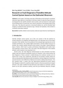
The error quaternions are illustrated in Fig. 1. They are all unit quaternions, i.e. have length one. For any measurable function u : [0, ∞ → Rn we define

and S(x) is the skew-symmetric cross-product operator matrix such that x1 × x2 = S(x1 )x2 .

7271

||u||∞ := sup |u(t)| t∈[0,∞

||u||a := lim sup |u(t)| (11) t→∞

qd

qf

ql ef

el q~l

eˆl

q~ f eˆ f

qˆ l Fig. 1.

qˆ f

Illustration of quaternion error variables

where each supremum is understood to be an essential supremum. The norm ||u||∞ is referred to as the L∞ -norm of u, while ||u||a is referred to as the asymptotic L∞ -norm of u. The initial value of a variable or function x will be denoted x0 . III. S YSTEM EQUATIONS The system equations are given by the kinematic differential equation (5) together with the dynamical equation: q˙ k =

1 i [ω ]q ⊗ qk 2 ik

(12)

d i i (J ω ) = τki (13) dt k ik where k = l for the leader and k = f for the follower. The last equation is the dynamics as seen from the inertial system, with Jik = Rk Jkk RTk where Jkk is the inertia matrix calculated in the k-frame, see [15]. Since the system does not move in the k-frame Jkk is constant. It can be shown that Jkk and Jik are symmetric and positive definite. The control is τki . The output of the system is qk , since it is assumed that the attitude is measured, whereas measurement of the i is assumed to be unavailable (see the angular velocity ωik Introduction). IV. C ONTROL OBJECTIVE The objective of the tracking/synchronization control is to design τfi and τli by output feedback control such that (1213) for k = l and k = f together with the observer dynamics presented in the next section give asymptotic convergence of ql to qd , and of qf to ql . We will call the problem of getting ql to track qd “the tracking problem”, while the problem of getting qf to track ql will be called “the synchronization problem”. These problems are different, because for the tracking problem the desired trajectory qd is given mathematically, while for the synchronization problem the desired trajectory is ql , which is a measured trajectory. For qd all higher order derivatives i can be calculated, and from this the angular velocity ωid of qd and all higher order derivatives of the angular velocity can be found. On the other hand, the angular velocity ωili of the desired trajectory in the synchronization problem is unavailable. This adds an extra difficulty to the problem, and implies that in the synchronization problem an observer must be used to estimate the angular velocity of the desired

trajectory. In addition comes that the angular velocity of the follower itself is not measured, such that we need an observer for this as well. The problem is thus an output feedback synchronization control problem. Also, since the angular velocity of the leader is not available, the problem of getting ql to track qd is an output feedback tracking control problem. Although there are differences between the tracking and synchronization problem the controller for both problems will be designed in a similar manner by the control design method presented in this paper. The control objective is therefore to use angular velocity observers and find control laws i i ˆl, ω ˆ ili ) , ω˙ id , . . . , ql , q τli = τli (qd , ωid

(14)

i ˆl, ω ˆ ili , qf , q ˆf , ω ˆ if τfi (ql , q )

(15)

τfi

=

such that el → ±1q and ef → ±1q , which implies ql → qd i ˆ ik and qf → ql . In (14-15) ω for k = l or k = f is the estimate of the angular velocity. The dots in (14) indicate that derivatives of any order may be used. However, we i . In Fig. will not use derivatives of higher order than ω˙ id 2 the structure of the system is shown. The input aD to the follower observer will be a function of the other variables and is therefore not included in (15). V. A NGULAR VELOCITY NONLINEAR OBSERVER In this section the observer used to estimate the angular velocities of the systems is presented. A nonlinear observer for estimation of angular velocity for rigid body motion was presented in [16]. This observer was modified in [17] in order to include different types of correction terms in the observer, and to give the error quaternion between system a and b in the a-coordinates instead of in the inertial coordinates as in [16]. We consider observers that have the following structure 1 i ˆ + g1k ] ⊗ q ˆk ˆ˙ k = [ω q 2 ik

(16)

d i i ˆ ) = τki + g2k (J ω (17) dt k ik where k = l for the leader and k = f for the follower. In the simulations we apply the observer presented in [17, Sec. 6.2], which has the form in (16-17) with (18) g1k (qk , zk ) := −Kv,k Rk zk 1 1 g2k (qk , zk ) := − kp,k (Jik )−1 Rk zk = − kp,k Rk (Jkk )−1 zk 2 2 (19) and zk = −

dH
˜k d˜ ηk

(20)

T where kp,k is a positive  v,k = Kv,k > 0. The  scalar,T K T ˜ k = η˜k
˜k .. observer error is q In [17] general properties that H must satisfy are given, and different choices for H are presented. One of the choices is  1 + η˜k for η˜k < 0 (21) H(˜ ηk ) = 1 − η˜k for η˜k ≥ 0 ⇒ zk = sgn(˜ ηk )˜
k (22)

7272

Output feedback synchronization control Output feedback tracking control

qd ωidi ω& idi

Fig. 2.

Leader Controller + System

ql

Leader Observer.

qˆ l ωˆ ili aD ≈ ω&ˆili

Follower Controller + System

qf

Follower Observer

qˆ f

ωˆ ifi

Leader-follower synchronization of attitude



where sgn(˜ ηk ) =

−1 for η˜k < 0 +1 for η˜k ≥ 0

(23)

which is the function used in the simulations in this paper. It is important to define the sgn-function as in (23), and not such that sgn(0) = 0 as this would lead to an extra equilibrium point for η˜k = 0. In [17, Sec. 6.2.1] a stability result was deduced for the use of any H-function with specified properties. We here state the theorem only for the H-function used in this paper: Theorem 1: If the observer given by (16-21) with g1k and g2k defined by (18-19), is applied to the system (12-13), it can be concluded that for any initial values of the attitude ˜ k → ±1q , which implies error and angular velocity error, q i i ˜ k converges asymptotically to I, and ω ˜ ik ˆ ik that R := (ω − i ) → 0. ωik From (16) it can be seen that the angular velocity of the estimated system is given by i ˆ ik + g1k ωiikˆ = ω

(24)

i ˆ ik is not equal Notice that the estimated angular velocity ω to the angular velocity of the estimated system. The control design presented in this paper may be used for any observer on the form (16-17). In the control design the only assumption about the observer will be Assumption 1: The observer is in the form (16-17), where the observer terms g1k , g2k are any expressions such that for any angular velocity of the observed trajectory, it can ˜ k → ±1q be shown that the observer errors are bounded, q i ˜ ik and ω → 0. This implies that g1k and g2k will converge to zero, since the observer dynamics must be equal to the actual dynamics after convergence of the observer errors.

VI. C ONTROLLER DESIGN A. Design method We propose a controller design based on vectorial observer backstepping [18], [19], in which backstepping design is applied to the observer equations. In [18] vectorial observer backstepping was applied to the design of nonlinear output feedback control of dynamically positioned ships. In [20] some comments to [18] were given in order to enlarge the method to a larger class of ships. In [21] a sliding mode observer (with the saturation function) was developed for a ship, and the vectorial observer backstepping method was

used to design the control input. In [22] a controller for attitude based on backstepping was developed, with full state feedback and for rest-to-rest maneuver. ˆf as error dynamics coordinates, and ˆl and e We choose e ˆl and e ˆf converge the controllers will be designed such that e to ±1q if an observer satisfying Ass. 1 is used. Another alternative would be to use el and ef as error coordinates ˆf lead to ˆl and e instead, but it was found that the use of e simpler design of the controller. For instance, the term (??) could not be calculated exactly if e := e1 or e := ef because the angular velocity of e would then be unknown. ˆl , e ˆf , q ˜ l and q ˜ f converge to From Fig. 1 it is seen that if e ±1q also el and ef converge to ±1q . This implies that ql → qd and qf → ql , which is the objective of the controller design. B. Error dynamics for the tracking/synchronization errors ˆl and This section presents the differential equations for e ˆf . From (5) and (6) it can be seen that the differential e ˆl is given by equation for e 1 d ˆ˙ l = [ωidˆl − ωid ˆl e ]q ⊗ e 2 1 i ˆl = [RTd (ωiiˆl − ωid )]q ⊗ e 2

(25)

By inserting for ωiiˆl from (24) with k = l (25) becomes 1 i ˆ ili − ωid ˆl ˆ˙ l = [RTd (ω + g1l )]q ⊗ e (26) e 2 ˆf can be written Similarly the differential equation for e as 1 ˆ ˆ ˆ˙ f = [ωilfˆ − ωilˆl ]q ⊗ e ˆf e 2 1 ˆT i ˆ −ω ˆ ili + g1f − g1l )]q ⊗ e ˆf = [R (ω (27) 2 l if ˆl and e ˆf are similar, except The differential equations for e ˆl is only influenced by the observer error for the leaderthat e ˆf is influenced by the observer errors of observer, while e both the observer for the leader satellite and the observer for the follower satellite. It is assumed that the observers satisfy Ass. 1. Since no assumptions about the trajectory to be observed is necessary for the observer, there is no coupling between the observer dynamics and tracking dynamics as was the case for synchronization of robots in [23]. The

7273

observer errors, and therefore g1f and g1l , can be treated as inputs to (26) and (27) with given bounds, and according to Ass. 1 g1f → 0 and g1l → 0. C. The controllers By using the equations (17), (26-27) we are able to design the output tracking controller for the leader and the output synchronization controller for the follower in a similar manner using vectorial observer backstepping. Both (26) and (27) are in the form 1 ˆ − ωD + vO )]q ⊗ e e˙ = [RT1 (ω (28) 2 with (17) in the form d ˆ = τ + g2 (Jω) (29) dt For the output feedback tracking problem of the leader ˆl , system (28) represents (26). This implies that e = e i ˆ = ω ˆ ili , ωD = ωid and vO = g1m . For the R1 = Rd , ω problem of output feedback synchronizing of the follower i ˆ l, ω ˆ =ω ˆ if ˆf , R1 = R , (28) represents (27). In this case e = e i ˆ il and vO = g1f − g1l . ωD = ω The term vO is a disturbance term caused by the observer errors. For both problems there is a bound for |vO | from the analysis of the observer, and vO goes to 0 as the observer errors go to zero. Equation (29) represents the observer equation (17). This i ˆ := ω ˆ ik gives that J := Jik , ω , τ = τki and g2 = g2k where k = l for the tracking problem of the leader and k = f for the synchronization problem. We also define J0 = Jkk , such that J = Rk J0 RTk . A difference between the tracking problem and the synchronization problem is that while for the tracking problem ω˙ D can be accurately calculated, this is not the case for the synchronization problem. For the synchronization of the ˆ˙ ili . However, from the observer follower to the leader ω˙ D = ω d ˆ ili ) = τli + g2l (Jil ω equations for the leader system only dt is known, and from this it is not possible to calculate ˆ˙ ili , because this requires knowledge of J˙ il that cannot be ω calculated since it depends on ωili . Using the idea of vectorial observer backstepping design ˆ as a virtual control for (28), and design τ such we choose ω ˆ converges towards a desired reference for the virtual that ω ˆ and define ˆ r be the desired ideal value for ω, control. Let ω ˆ as the tracking error for ω ˆ =ω ˆr + s ˆ −ω ˆr ⇒ ω s=ω

(30)

By inserting (30) into (28) the dynamics of e become 1 ˆ r − ωD + s + vO )]q ⊗ e (31) e˙ = [RT1 (ω 2 We define the reference trajectory as ˆ r = R1 α1 (e) + ωD ω

(32)

ˆ r implies where α1 (e) is defined later. The definition of ω that (31) becomes 1 (33) e˙ = [α1 (e) + RT1 (s + vO )]q ⊗ e 2

In Section VII the dynamics in (33) is analysed and possible choices of α1 (e) are given such that e → ±1q if |s|,|vO | are bounded and s, vO → 0 as t → 0. We assume that α1 (e) is defined as in Section VII. The aim of the control design is then to find a control such that the dynamics of s is asymptotically stable. The dynamics of vO is asymptotically stable as shown by the observer analysis. d ˆ r ) was exactly known we could define the control If dt (Jω as d ˆ r ) − As Js τideal = −g2 + (Jω (34) dt with As = ATs > 0. From (29) it is seen that the closed loop system would then be d (Js) = −As Js (35) dt which would give convergence to zero of Js, and therefore d ˆ r ) is unknown, (Jω of s, since J is non-singular. However, dt both for the tracking problem and the synchronization problem, since J˙ is unknown. For the synchronization problem ˆ˙ r is unknown. It is therefore difficult to design a also ω controller such that s → 0 no matter what the observer errors are. We therefore design a controller such that the dynamics of s depend on the observer errors, but still s → 0 as t → ∞, under Ass. 1 for the observer. This will be done by finding an approximation to the expression in (34) such that the approximation error go to zero as the observer errors converge. We propose to use an approximation ω˙ D ≈ aD in the synchronization problem, where the expression for aD is given in the Appendix. The approximation is such that ω˙ D = aD + δD

(36)

˜ ili goes where the approximation error δD goes to zero as ω to zero. To use the same equations for both the tracking problem and the synchonization problem we define δD = 0 i for the tracking problem. and aD = ω˙ D := ω˙ id By differentiating (32) and using (36) it is seen that d ˆ˙ r = ar + δD with ar = (R1 α1 (e)) + aD (37) ω dt where ar is known, since aD and the angular velocity of R1 , e˙ are known. From (62-63) we get d ˆ r ) = Jω ˆ˙ r + (LJ (ω, ˆ J) − LJ (ω, ˜ J))ω ˆr (Jω (38) dt where LJ is an operator defined by (62). We now use (37-38) to propose the following approximation to the ideal controller in (34) ˆ J)ω ˆ r − As Js τ = −g2 + Jar + LJ (ω,

(39)

For the theoretical analysis the control in (39) can be written as ˜ J)ω ˆr τ = τideal − JδD + LJ (ω,

(40)

˜ J) converge to zero as the observer error Both δD and LJ (ω, for the angular velocity converges to zero.

7274

˜ J)ω ˆ r the By defining z1 = Js and w1 = −JδD + LJ (ω, closed loop dynamics become z˙ 1 = −As z1 + w1

(41)

One may also remove g2 from (39) and instead add it to w1 , since also g2 converge to 0 under Ass. 1. Use of the Lyapunov function Vz = 12 zT1 z1 and the theorem about uniform ultimated boundedness, [24, Th. 4.18], gives that ||z1 ||∞ ≤ max{βz (|z0 |, t − t0 ),

||w1 ||∞ } Asm

(42)

where βz is a class-KL function and Asm is the smallest eigenvalue of As . It is possible to choose βz (|z10 |, 0) ≤ 1 ||∞ |z10 |, since if |z10 | ≥ ||w it can be seen that Vz Asm decreases, which implies |z1 | < |z10 |. Using time invariance and the bound on ||z1 ||∞ it can be shown from (42) that ||z1 ||a =

||w1 ||a Asm

(43)

see [25, p. 1258]. We know from the analysis of the observer that ||w1 ||a = 0, and therefore we have now shown that ||z1 ||a = 0, which implies ||s||a = 0 since J is nonsingular. We now return to the analysis of (33). We have just shown that the dynamics of s is asymptotically stable and from the analysis of the observer we also have that vO → 0 as t → ∞. This together with Th. 3 gives the following result: Theorem 2: If the controller given by (39) with α1 (e) as defined in Th. 3 is applied to the system (28-29), and the states of the leader and follower are estimated by an observer satisfying Ass. 1, then e → ±1q for any initial value such that |e0 | = 1. This implies global asymptotic stability of R(e) = I. ˆl for the tracking problem of the leader We have e = e ˆf for the synchronization problem of the follower, and e = e but are mainly interested in showing that el → ±1q and ef → 1q . Fig. 1 shows that ˆl ⊗ q ˜ −1 el = e l ˜l ⊗ e ˆf ⊗ ef = q

˜ −1 q f

(44)

We can look at Hα either as a function of |
e | or as a function of ηe . A possible choice of Hα is given by (21), which comes from the choice V (u) = u. Let α1 in (46) be chosen as dHα α1 (e) = Λ1
e (50) dηe with Λ1 = ΛT1 > 0. We have that dHα dV (ue ) = −sgn(ηe ) (51) dηe due The above definition of α1 and (46) implies that if |∆ω| → 0 as t → ∞ then e → ±1q . Since both e = 1q and e = −1q correspond to the rotation matrix Re = I there is no attitude error as t → ∞. Proof: Because ηe2 + |
e |2 = 1 for all time we can use only |
e | or only |ηe | in the analysis. We will look at Hα as a function of |
e | because Hα is a positive definite function of |
e |, and can therefore be used as a Lyapunov function. However, it is a decreasing function of |ηe |. We have that dHα dHα d|
e | = H˙ α = η˙ e d|
e | dt dηe

(45)

ˆf , q ˜ l and q ˜ f converge to ±1q ˆl , e This implies that as e also el and ef converge to ±1q . VII. A NALYSIS OF THE ATTITUDE ERROR From the analysis in the last section it is seen that the differential equation for the attitude error is given by (33): 1 [α1 (e) + ∆ω]q ⊗ e with ∆ω = RT1 (s + vO ) (46) 2 In this section possible choices of α1 are given such that e → ±1q as t → ∞ if ∆ω → 0. If ||∆ω||∞ is smaller than a value defined later and |
e0 | < 1 we in addition find a bound for ||
e ||∞ which is smaller than the a priori bound of 1. The following Lemma is a well known fact which will be used in the analysis e˙ =

Lemma 1: For any ωe := α1 (e) + ∆ω (46) gives that if the initial value |e0 | = 1 we get |e| = 1 ∀t, and therefore ηe2 ≤ 1 ∀t and |
e |2 ≤ 1 ∀t. Proof: By differentiating lx := ηe2 +
Te
e = |e|2 along the trajectories of (46) we get 1 1 l˙x = 2ηe (− ωeT
e ) + 2
Te [ηe ωe − S(
e )ωe ] = 0 (47) 2 2 and therefore lx is constant. We always have |e0 | = 1 because it is a unit quaternion from the definition of e0 . The following Theorem defines some possible choices of α1 (e): Theorem 3: Let V (u) be a strictly increasing function defined on [0, 1] and let V (0) = 0. Assume that V has a bounded derivative such that dV (u) ≤ k2 k1 ≤ (48) du for all u ∈ [0, 1]. Define  Hα = V (ue ) with ue := 1 − 1 − |
e |2 = 1 − |ηe | (49)

(52)

Although we look at Hα as a function of |
e | we will calculate the derivative by the last expression in (52), because this is somewhat simpler. Because we have |e| = 1 ∀t from Lemma 1 we know that ue ≤ 1 ∀t which implies Hα ≤ V (1) ∀t. Define ||∆ω||[t1 ,∞ = supt∈[t1 ,∞ |∆ω|

(53)

From the assumption |∆ω| → 0 as t → 0 we have that ||∆ω||[t1 ,∞ → 0 as t1 → 0. For t ≥ t1 where t1 is any time larger than the initial time t0 we get from (46), (50) and (2) :    dHα dHα 1 H˙ α = Λ1
e + ∆ω (54) −
Te dηe 2 dηe 1 ≤ − |
e |(k12 Λ1m |
e | − k2 ||∆ω||[t1 ,∞ ) (55) 2

7275

We see that H˙ α ≤ −WH (|
e |) where WH is a positive definite function if k2 ||∆ω||[t1 ,∞ := µt1 (56) |
e | > k12 Λ1m

(57)

we have that H˙ α ≤ −WH (|
e |) for Hα (|
e |) > Hα (µt1 ), and therefore Hα decreases until ultimately Hα (|
e |) ≤ Hα (µt1 ) ⇒ |
e | ≤ µt1

(58)

The arguments above are from [24, Th. 4.18]. By letting t1 → ∞ in the above analysis we get µt1 → 0 and therefore |
e | → 0, which by using |e| = 1 implies ηe → ±1, and therefore e → ±1q . If ||∆ω||∞ and |
e0 | are small we can find a smaller bound than 1 for |
e | during the transient response, by using the following theorem: Theorem 4: If k2 ||∆ω||∞ µt0 := µt0 we will have H˙ α < 0 until |
e0 | ≤ µt0 , and this implies that for |
e0 | > µt0 Hα (|
e |) < Hα (|
e0 |) ⇔ |
e | ≤ |
e0 |. This implies the bound in (60).

VIII. S IMULATION A simulation was performed in order to validate the method. The inertia matrices were set to Jll = Jff = diag(5.3, 6.0, 6.7). The observer gains for the observer in Sec. V were Kv,l = Kv,f = 2I and kp,l = kp,f = 0.7. The function α1 (e) was defined as in (50) for both the leader and the follower with Λ1 = 0.5I for both. The control input was as in (39) with As = 0.5I for both the leader and the follower, but without the g2 term as explained below (39). The gains were chosen so low because low available torque has been assumed, since the maximum available torque from thrusters and reaction wheels is mostly not higher than 0.05 Nm for small satellites. Band-limited white noise was added to the measurements of the attitudes in order to simulate measurement noise. This was done by adding band-limited white noise with standard deviation σ = 0.01 to each  component of
and calculating η with noise as ηn = 1 −
Tn
n , where
n is the vector part of the quaternion after noise is added. Since 2 arcsin(0.01) ≈ 1◦ , this corresponds with an error of about

1 0.62 0.62 0.8 0.8

2 0.35 0.35 0.5 0.5

3 0.5771 0.5771 0.2646 0.2646

ω1 1e − 4 0 2e − 4 0

ω2 5e − 5 0 4e − 4 0

ω3 3e − 4 0 15e − 4 0

TABLE I I NITIAL VALUES , L: L EADER , LO: O BSERVER FOR THE LEADER , F: F OLLOWER , FO: O BSERVER FOR THE FOLLOWER .

1◦ in the measurement of angles. The noise was different on each element. The desired attitude for the leader was given by ˜ 1 (t) with q1 = [ 0.3 0.7 0.4 0.5099 ]T qd (t) = q1 ⊗ q θ(t) T T . The rota˜ 1 (t) = [ cos( θ(t) and q 2 ) sin( 2 )k ] tion axis k was constant and defined by kT = − t [ 0.1574 0.9861 −0.0551 ] and θ(t) = θTMθ e Tθ with θM = π/3 and Tθ = 60 seconds. The initial values are shown in table I. We assume that the synchronization scheme starts after detumbling of the satellites, and therefore it is known that the initial angular velocity of each satellite is small. In Fig. 3 the results for the quaternion elements of the desired attitude, the leader attitude and the follower attitude are shown. The control torque varied between ±0.02 Nm after the transient response, and between ±0.15 Nm during the transient response. In order to have torques smaller than ±0.05 Nm all the time one would therefore have to use smaller gains during the transient response, and the response would then take longer time. Before t = 55 seconds the attitudes are plotted without the added noise, since we want to see how well the actual trajectories converge to each other. In Fig. 4 the rotation angle corresponding with the tracking error el for the leader, and synchronization error ef for the follower is shown after the

transient response. It was calculated by θk = 2 arcsin(
Tek
ek ) for k = l, f . The angle is higher for the synchronization than for the tracking, but we see that in both cases the angle is small. It was seen that el ≈ 1q and ef ≈ 1q . With other initial values we got convergence to −1q . 1 desired leader follower

0.9 0.8

ε3

0.7

ε1

0.6

ε

2

0.5 0.4

k

Hα (|
e |) > Hα (µt1 ) ⇒ |
e | > µt1

η 0.4 0.4 0.2 0.2

q (i), i=1,2,3,4, k=d,l,f

Choose t1 so large that µt1 < 1. This is possible because of the assumption ||∆ω||[t1 ,∞ → 0 as t1 → ∞. For µt1 > 1 (56) is never satisfied because |
e | ≤ 1. We know that Hα ≤ V (1) ∀t, and therefore Hα is bounded for t = t1 , and we can start the analysis at t1 instead of at t0 . Since

L LO F FO

0.3

η

0.2 0.1 0

0

10

20

30 time [s]

40

50

60

Fig. 3. Quaternion elements for the desired attitude, leader and follower . Before t = 55 minutes the attitudes are plotted without the added noise

7276

θl

Rotation angle for el and ef [degrees]

0.35

θf

0.3 0.25 0.2 0.15 0.1 0.05

30

35

40

45

50 time [s]

55

60

65

70

Fig. 4. Rotation angle corresponding with el and es , calculated from the actual values (before the noise is added).

IX. C ONCLUSION A scheme for output feedback synchronization of the attitude of two satellites was developed, and the results were validated by simulation. It was shown by analysis that the rotation matrix for the attitude error converges to the identity matrix for any initial values. This was confirmed by the simulations. A PPENDIX ˆ˙ ili D EDUCTION OF AN APPROXIMATION TO ω We have d J˙ il = (Rl Jll RTl ) = S(ωili )Jil − Jil S(ωili ) dt ˜ ili )Jil − Jil S(ω ˆ ili − ω ˜ ili ) ˆ ili − ω = S(ω

(61)

By defining the operator LJ (ω, J) = S(ω)J − JS(ω)

(62)

ˆ ili , Jil ) − LJ (ω ˜ il , Jil ) J˙ il = LJ (ω

(63)

(61) becomes

where the first term is known and the second term goes to zero as the observer errors go to zero. From d i i ˆ ) = τli + g2m (J ω dt l il ˆ˙ ili + (LJ (ω ˆ ili , Jil ) − LJ (ω ˜ il , Jil ))ω ˆ ili = τli + g2l Jil ω ˆ˙ ili = aD + δD with we get ω˙ D = ω  ˆ ili , Jil )ω ˆ ili aD = (Jil )−1 τli + g2l − LJ (ω δD =

˜ ili , Jil )ω ˆ ili (Jil )−1 LJ (ω

(64)

(65) (66)

R EFERENCES [1] D. Scharf, F. Hadaegh, and S. Ploen, “A survey of spacecraft formation flying guidance and control (part II): Control,” in Proccedings of the 2004 American Control Conference, Boston, MA, 2004, pp. 2976– 2985. [2] P. K. C. Wang and F. Hadaegh, “Coordination and control of multiple microspacecraft moving in formation,” The Journal of the Astronautical Sciences, vol. 44, pp. 315–355, 1996.

[3] P. Wang, F. Hadaegh, and K. Lau, “Syncronized formation rotation and attitude control of multiple free-flying spacecraft,” Journal of guidance, control and dynamics, vol. 22, no. 1, pp. 28–35, 1999. [4] R. W. Beard, J. Lawton, and F. Y. Hadaegh, “C coordination architecture for spacecraft formation control,” IEEE Transactions on control systems technology, vol. 9, pp. 777–790, November 2001. [5] J. T.-Y. Wen and K. Kreutz-Delgado, “The attitude control problem,” IEEE Transactions on automatic control, vol. 36, no. 10, pp. 1148– 1162, 1991. [6] H. Pan and V. Kapila, “Adaptive nonlinear control for spacecraft formation flying with coupled translational and attitude dynamics,” in Proceedings of the 40th IEEE Conference on Decision and Control, Orlando, Fl, 2001, pp. 2062–2067. [7] B. Costic, D. Damon, M. de Queiroz, and V. Kapilia, “A quaternionbased adaptive attitude tracking controller without velocity measurements,” in Proceedings of the 39th IEEE Conference on Decision and Control, Sydney, Australia, 2000, pp. 2429–2434. [8] Q. Yan, G. Yang, V. Kapila, and M. de Queiroz, “Nonlinear dynamics and output feedback control of multiple spacecraft in elliptical orbits,” in Proceedings of the American Control Conference, Chicago, Illinois, 2000, pp. 839–843. [9] F. Lizarralde and J. T. Wen, “Attitude control without angular velocity measurement: a passivity approach,” IEEE Transactions on automatic control, vol. 41, no. 3, pp. 468–472, March 1996. [10] J. Lawton and R. Beard, “Synchronized multiple spacecraft rotations,” Automatica, vol. 38, pp. 1359–1364, 2002. [11] W. Kang, N. Xi, and A. Sparks, “Theory and applications of formation control in a perceptive reference frame,” in Proceceedings of the 39th IEEE Conference on Decision and Control, Sydney, Australia, 2000, pp. 352–357. [12] W. Kang and H.-H. Yeh, “Co-ordinated attitude control of multisatellite systems,” International journal of robust and nonlinear control, vol. 12, pp. 185–205, 2002. [13] K. K¨opr¨ubasi and M.-W. L. Thein, “Spacecraft attitude and rate estimation using sliding mode observers,” in Proceedings of International Conference on Recent Advances in Space Technologies, 2003, pp. 169– 173. [14] J. B. Kuipers, Quaternions and rotation sequences. Princeton university press, Princeton, New Jersey, 1999. [15] O. Egeland and J. T. Gravdahl, Modelling and Simulation for Automatic Control. Marine Cybernetics, Trondheim, Norway, 2002. [16] S. Salcudean, “A globally convergent angular velocity observer for rigid body motion,” IEEE Transactions on automatic control, vol. 36, no. 12, pp. 1493–1497, 1991. [17] O.-E. Fjellstad, “Control of unmanned underwater vehicles in six degrees of freedom: a quaternion feedback approach,” Doktor Ingeniøravhandling, Report 94-92-W, Department of Engineering Cybernetics, The Norwegian institute of Technology, University of Trondheim, Norway, November 1994. ˚ Grøvlen, “Nonlinear output feedback control of [18] T. I. Fossen and A. dynamically positioned ships using vectorial observer backstepping,” IEEE Transactions on control systems technology, vol. 6, no. 1, pp. 121–128, 1998. [19] M. Krstic, I. Kanellakopoulos, and P. Kokotovic, Nonlinear and Adaptive Control Design. John Wiley & Sons., Inc., 1995. [20] A. Robertsson and R. Johansson, “Comments on ”nonlinear output feedback control of dynamically positioned ships using vectorial observer backstepping*”,” IEEE Transactions on control systems technology, vol. 6, no. 3, pp. 439–441, 1998. [21] M.-H. Kim and D. J. Inman, “Development of a robust non-linear observer for dynamic positioning of ships,” Proceedings of the institution of mechanical engineers part I - Journal of systems and control engineering, vol. 218, no. 1, pp. 1–11, 2004. [22] J. Lu and B. Wie, “Nonlinear quaternion feedback control for spacecraft via angular velocity shaping,” 1994, proceedings of the American Control Conference, Baltimore, Maryland. [23] A. K. Bondhus, K. Y. Pettersen, and H. Nijmeijer, “Master-slave synchronization of robot manipulators,” 2004, iFAC Symposium NOLCOS 2004, Symposium on Nonlinear Control Systems. [24] H. H. Khalil, Nonlinear Systems, 3rd ed. Prentice Hall, 2002. [25] A. R. Teel, “A nonlinear small gain theorem for the analysis of control systems with saturation,” IEEE Transactions on Automatic Control, vol. 41, no. 9, pp. 1256–1270, September 1996.

7277