Acknowledgements The authors would like to thank the Gates Cambridge Trust, the Over- seas Research Scholarship Programme the EPSRC, and the Gottlieb ...
Learning a Kinematic Prior for Tree-Based Filtering A. Thayananthan
P. H. S. Torr †
B. Stenger
University of Cambridge Dept. of Engineering Cambridge, CB2 1PZ, UK
R. Cipolla
†
Microsoft Research Ltd. 7 JJ Thompson Avenue Cambridge, CB3 OFB, UK
Abstract
The aim in this paper is to track articulated hand motion from monocular video. Bayesian filtering is implemented by using a tree-based representation of the posterior distribution. Each tree node corresponds to a partition of the state space with piecewise constant density. In a hierarchical search regions with low probability mass can be rapidly discarded, while the modes of the posterior can be approximated to high precision. Large sets of training data are captured using a data glove, and two techniques for constructing the tree are described: One method is to cluster the collected data points using a hierarchical clustering algorithm, and use the cluster centres as nodes. Alternatively, a lower dimensional eigenspace can be partitioned using a grid at multiple resolutions, and each partition centre corresponds to a node in the tree. The effectiveness of these techniques is demonstrated by using them for tracking 3D articulated hand motion in front of a cluttered background.
1 Introduction Tracking articulated hand motion is a challenging problem, particularly if only a single view is to be used. This problem is mostly approached using differential tracking methods, where the object pose in the current frame is estimated from the state in the previous frame. Because there is much ambiguity in tracking articulated objects, it is important to maintain multiple hypotheses [8, 17]. Tracking articulation is often done in the context of human body tracking for which there exists a large amount of literature.Some body trackers model the dynamics explicitly, for example using a switching linear dynamic system [11]. It is difficult to learn such a model for hand motion, because there are no obvious motion patterns such as walking or running. Currently, most trackers use particle filtering [7], in which it is essential to be able to sample from the prior to generate new hypotheses. With the increase in computational power one may also consider handling ambiguous situations by treating tracking as object detection in each frame. Thus if the target is lost in one frame, this does not affect the subsequent frame. Furthermore template based methods have yielded good results for locating deformable objects in a scene with no prior knowledge, e.g. for hands or pedestrians [1, 3]. These methods are made efficient by the use of distance transforms to compute the chamfer or Hausdorff distance between template and image [2, 6]. Multiple
BMVC 2003 doi:10.5244/C.17.60
templates can be dealt with efficiently by building a tree of templates [3, 10]. However, exhaustive search for the object is computationally expensive and results in jerky motion. The question is therefore how to include dynamic information. Within this paper techniques are proposed to generate templates which are derived from learned object intrinsic motion: Data sets are captured using a data glove, and a three-dimensional hand model is used to generate templates by projecting it into the image. The next section gives a short review of Bayesian filtering and motivates the use of a tree-based filtering algorithm, introduced in [13]. In section 3 it is shown how a motion prior based on hand kinematics can be used within this framework. The likelihood function is derived in section 4, and section 5 shows tracking results on a video sequence of articulated hand motion.
2 Tree-Based Filtering This section briefly reviews the technique of tree-based filtering, which is described in more detail in [13]. The tracking problem is formulated within a Bayesian filtering framework: Define, at time t, the state parameter vector as θ t , and the data (observations) as Dt , with D1:t � 1 , being the set of data from time 1 to t � 1; and the data D t are conditionally independent at each time step given the θ t . In our specific application θ t is the state of the hand (set of joint angles) and D t is the image at time t or a set of features extracted from that image. Thus at time t the posterior distribution of the state vector is given by the following recursive relation
�
�
�
p θ t � D1:t ���
p Dt � θ t � p θ t � D1:t � � p Dt � D1:t � 1 �
�
where the prior from the previous time step, p θ t � D1:t �
�
p θ t � D1:t �
�
1
� �
�
p θt � θt�
1
1
1
�
(1)
�
� , is obtained by
� � p θ t � 1 � D1:t � 1 � d θ t �
1
�
(2)
with the initial distribution p θ 0 � D0 � assumed known. The evaluation of equation (2) is also known as prediction step, and equation (1) is the measurement update step. However, these equations are intractable for all but certain simple distributions and so approximation methods have to be used. Monte Carlo methods such as particle filtering [5, 7] represent one way of evaluating the terms. Our suggested approach, which has shown to be effective, is based on hierarchical partitioning of the state space. A tree is constructed in which each node represents a partition of the state space. Figure 1(a) shows a schematic example of such a tree. The posterior distribution is encoded using a piecewise constant distribution over the leaves of the tree. This distribution will be mostly zero for many of the leaves. The likelihood is evaluated by using the centre of each partition, i.e. the hand model in a particular configuration, to generate a template which can be compared to the image. Kinematic information is incorporated by learning state transition distributions. The search is made efficient by only evaluating sub-trees with high posterior probability, but care has to be taken when setting the thresholds for these decisions so as to not discard good hypotheses too early.
�
pθD
l =1 θ
�
pθD
l =2
θ
PSfrag replacements p � θ D l =3 θ
(a)
(b)
Figure 1: Tree-based estimation of the posterior density (schematic). (a) Associated with the nodes at each level is a partition of the state space (here the coefficient of the first principal component of joint angles, see section 3). The posterior for each node is evaluated using the centre of each partition, depicted by a hand in a certain configuration. Sub-trees of nodes with low posterior are not further evaluated. (b) Corresponding posterior density (continuous) and the piecewise constant approximation using tree-based estimation. The modes of the distribution are approximated with higher precision at each level. Comparison to Tree-Based Detection A common way to build a tree of templates is to cluster templates using a similarity measure [3, 10]. The idea is to group similar templates and represent them with a single prototype template together with an estimate of the variance of the error within the cluster, which is used to define a matching threshold. The prototype is first compared to the image; only if the error is below the threshold are the templates within the cluster compared to the image. This clustering is done at various levels, resulting in a hierarchy, with the templates at the leaf level covering the space of all possible templates. However, it is not straightforward to incorporate a motion prior for the templates. For example, consider the case in figure 2, where two hand poses which are far apart in parameter space yield two similar templates. These templates may be clustered together, even though they have different motion priors. When building the tree in parameter space, however, the two configurations are very likely to be in different sub-trees, allowing for different priors. In order to use the tree-based filter, some questions need to be addressed: How � should the state space be partitioned? How do we obtain state transition probabilities p θ t � θt� 1� ? � Finally, what is a suitable likelihood function p D t � θ t � ? The answers to the first two questions will be based on a model of the hand kinematics, described in the following section.
(a)
(b)
Figure 2: Poses of the hand with large parameter distance yet similar shape. Two poses of an open hand, which have large distance in the rotation space (180 degrees) but project to similar shapes. Clustering based on shape similarity may group them together, whereas partitioning of the state space will not, allowing different motion priors.
3
Modelling Hand Kinematics
Model-based trackers commonly use a 3D geometric model with an underlying biomechanical deformation model to represent the hand [1, 12]. Each finger can be modelled as a kinematic chain with 4 degrees of freedom (DOF), and the thumb with 5 DOF. Thus articulated hand motion lies in a 21 dimensional joint angle space. Given a 3D hand model, inverse kinematics may be used to calculate the joint angles [16], however this problem is ill-posed when using a single view and it requires exact feature localization, which is particularly difficult in the case of self-occlusion. Hand motion is highly constrained as each joint can only move within certain limits. Furthermore the motion of different joints is correlated, for example, most people find it difficult to bend the little finger while keeping the ring finger fully extended at the same time. Thus hand articulation is expected to lie in a compact region within the 21 dimensional angle space. Previous Work In [17] Wu et al. use PCA to project the 20 dimensional joint angle measurements into a 7D subspace, capturing over 95 percent of the variation in the data set. Zhou and Huang [18] project the data into a 6D subspace, capturing over 99 percent of variation of a smaller training set. In both cases, valid finger configuration define a compact region within the subspace, and the goal is to sample from this region. One approach, adopted by Wu et al., is to define 28 basis configurations in the subspace, corresponding to each finger being either fully extended or fully bent (not all 2 5 � 32 combinations of fingers extended/bent are used). It is claimed that natural hand articulation lies largely on linear 1D manifolds spanned by any two such basis configurations, and sampling is implemented as a random walk along these 1D manifolds. Another approach [18] is to train a linear dynamic system on the region while decoupling the dynamics for each finger. In this case one motion sample corresponds to five random walks along 2D curves, each random walk corresponding to the motion of one particular finger. In [13] the nonlinear manifold of valid motions is approximated with a piecewise linear function. This is done separately for each finger, thus the correlation between movements of different fingers is not captured. In a number of experiments with 15 sets of joint angles (sizes of data sets: 3,000 to
(a)
(b)
Figure 3: Paths in the eigenspace. (a) The figure shows a trajectory of projected hand state (joint angle) vectors onto the first three principal components. (b) The hand configurations corresponding to the four end points in (a). 264,000) captured from three different subjects carrying out a number of different hand gestures, we found in all cases that 95 percent of the variance was captured by the first eight principal components, in 10 cases within the first seven, which confirms the results reported in [17]. However, except for very controlled opening and closing of fingers, we did not find the one-dimensional linear manifold structure reported in [17]. For example, figure 3 shows trajectories (projected onto the first three eigenvectors) between a subset of basis configurations used in [17]. The hand moved between the four basis configurations in random order for the duration of one minute. It can be seen that even in this controlled experiment the trajectories between the four configurations do not seem to be adequately represented by 1D manifolds. Tree Building by Clustering In order to build the tree described in section 2, the state space needs to be partitioned at multiple resolutions. One way to do this is to cluster the data using a hierarchical k-means algorithm, using the L 2 distance measure. This algorithm is also known as the generalised Lloyd algorithm in the vector quantisation literature [4], where the goal is to find a number of prototype vectors which are used to encode vectors with minimal distortion. Note that if the distance measure is an appearance based distance, such as chamfer distance, one would obtain a detection tree as described in section 2. The cluster centres obtained in each level of the hierarchy are used as nodes in one level of the tree. A partition of the space is given by the Voronoi diagram defined by these nodes, see figure 4a. Tree Building by Partitioning the Eigenspace Another way to subdivide the space is to use a regular grid. Defining partition boundaries in the original 21 dimensional space is difficult though, because the number of partitions increases exponentially with the number of divisions along each axis. Therefore the data can first be projected onto the first k principal components (k � 21), and the partitioning is done in the transformed parameter space. The centres of these hyper-cubes are then used as nodes in the tree on one level, where only partitions need to be considered which contain data points, see
λ2
θ2
PSfrag replacements
%�%& ��¸¹�� º�º ,- ./ 0��� 01 23 U�T UT RS PQ »�»$%��� �� ��� �� �&' �� ¼½ �� () 54 BC DE VW ·�@A )* · �� 6�7�FG+, H�I�67 HI � L�M LMNOJK ø X�ø -�XY Z[ - õ #�#$ bc ? < '( < d�d � ù�÷�ö ù÷ö .�. ô�"�ô " ²�ñ�ð ²³��ñð òó jk ih�ihlm ´�´µ Ë�Ê È�� 89 ËÊ ÈÉÒ�f�ÐÎ n�ÍÌ ÒÓ fgÐÑÎÏ üý à�áno Ý�Ü úûÚ�¶�àá â�ÝÜ þÿ ÚÛ > ¶ âã =�t�u = e�tu � e s�r :; sr ¦§ ¾�¾¿ pq ���� � "�!!�"!! ÀÁ ;< °±"# � �� /�/0 12 �¥�¤
replacements ÆÇìí ! Ä�êë �ÄÅ �� ßÞ ßÞ � ��vw �PSfrag ¥¤ Â�ÂÃ*+ 9: îï ×^_ �Ö ÔÕ ×Ö ¨©� ª�`�ª« æç `a èé äå� ØÙ ¬� |} ~ \] �� ®¯ ��34 5��� 56 � ¡ ¢£ θ1 �� ���� �� ��� 78 y�x yx z{ θ 2
âã MN � Þß O�OP o>n on QR JK ÔÕ z{ �� �� EED HI àá ÈÉ ¨>xy ¨© ª>FG ª« p>pq +, PQ ¬¬ ÒÓ > ê ë ê � UV ·>¶ ·¶ CD îï gh f�e å>ä i�fe åä ij LMM BC ?>= D KL ?= ü>Ý>Ü21 üý ÝÜ WX >Æ> ÆÇ ìí f�e fe UT>UT ¤¥ � L >VW ;< ¸¹ ¦§ 8�7 5�º» 87 56 0/ .--. ÚÛ v>��� ØÙ !" vw £>¢ �� ÐÑ O>N £¢ ²>¼>ON ÿ>þ ²³ ¼½ >ÿþ´> ¡ rs ´µ \] Z>Z[ >>%& @A Y>X #$ YX > 9: 34 ��� �� �� ��¿ �� => EF èéæ>æç IJ
^>> l>^_ °±lm > ®¯ cd`>bc `a (�' (' ��� �� ]^ ¾¾¿ ��~>�� ~ [�[\ |} @�? @? � S ÀÁ �� �� ÌÍ ñ>ð ñð òó )* fg ôõ ÷öö÷ RRS Ë Â>Âà Ê>Ê>_` ÊËÊ B�A BA i h k j H�G HG d>de ab úû øù
θ1
tuut �� TS ÏÎÎÏ ÄÅ Ö× YZ
λ1
(b)
(a)
Figure 4: Partitioning the State Space. This figure illustrates two methods of partitioning the state space: (a) by clustering the data points in the original space, and (b) by first projecting the data points onto the first k principal components and then using a regular grid to define a partition in the transformed space. The figure only shows one level of a hierarchical partition, corresponding to one level in the tree. figure 4b. Multiple resolutions are obtained by subdividing each partition. � Given the partition of the space, the state transition distributions p θ t � θ t � 1 � can be modelled as a Markov process. We model it as a first order process, and compute the transition probabilities by histogramming transitions in the training set. Given a large amount of training data, higher order models can be learned. Nonlinear Dimensionality Reduction In general the trajectories in eigenspace are nonlinear. Figure 5 shows an example of slightly more complex finger articulation, the trajectories in configuration space which are generated by spelling “BMVC” in American sign language. Thus techniques for nonlinear dimensionality reduction, such as the Isomap [14] algorithm, may turn out to be more suitable to analyse the data. The Isomap algorithm is an extension of multidimensional scaling (MDS), In MDS the objective is to maintain pairwise distances between data points while reducing the dimensionality. Isomap uses approximate geodesic distances (trajectories on the manifold), computed from a locally connected graph, instead of Euclidean distances between data points. We have applied the Isomap algorithm to a number of data sets, but experiments show that the results are very dependent on choosing the right local distances to compute the pairwise distances. This is difficult, because some parts of the joint angle space are more densely sampled than others.
4
Formulating the Likelihood �
The likelihood function p D t � θ t � relates the observations Dt to the unknown state θ t . For hand tracking, finding good features is challenging, since there are few features which can be detected and tracked reliably. Colour values and edges contours have been used in the past [1, 8, 17]. Thus the data is taken to be composed of two sets of observations, those
(a)
(b)
Figure 5: Paths in the configuration space found by PCA are nonlinear. (a) The figure shows the trajectory of projected state vectors onto the first three principal components, (b) the corresponding motion is the American sign language spelling of “BMVC”. from edge data Dtedge and from colour data D tcol . The log likelihood function used is
�
�
log p Dt � θ t � � log p Dtedge � θ t �
k
�
λ log p Dtcol � θ t �ml
(3)
�
where λ is a weighting parameter. The term for edge contours p D tedge � θ t � is based on theo chamfer distance function [2]. Given the set o of mprojected model contour points n n r and the set of Canny edge points u i p iq 1 � v j p j q 1 , a quadratic chamfer distance � function is given by �n 1 n 2� 2 dcham r ��� d i r � (4) n i∑ � � � q 1
�
� � � max minv j sut � � ui � v j � � τ � is the thresholded distance between the point, � � , and its closest point in r . Using a threshold value τ makes the matching more
where d i r n
ui v robust to outliers and missing edges. The chamfer distance between two shapes can be computed efficiently using a distance transform, where the template edge points are correlated with the distance transform of the image edge map. Toyama and Blake [15] show how the quadratic chamfer function can be turned into a likelihood which is approximately Gaussian. Edge orientation is included by computing the distance only for edges with similar orientation, in order to make the distance function more robust [10]. We also exploit the fact that part of an edge normal on the interior of the contour should be skin-coloured, and only take those edges into account� [8]. In constructing the colour likelihood function p D tcol � θ t � , we seek to explain all the image pixel data given the proposed state. Given a state, the pixels in the image w are partitioned into a set of object pixels x , and a set of background pixels y . Assuming pixel-wise independence, the likelihood can be factored as
�
p Dtcol � θ t �
�
�
� �
� �
∏ p It o� � θ t � ∏ p It b� � θ t � �
o s{z
(5)
b s}|
where It k � is the intensity normalised rg-colour vector at pixel location k at time t. The object colour distribution is modeled as a Gaussian distribution in the normalised colour
space. The object color distribution is modeled as a Gaussian distribution in the normalized color space, for background pixels a uniform distribution is assumed. For efficiency, we evaluate only the edge likelihood term while traversing the tree, and incorporate the colour likelihood only at the leaf level.
5
Results
We demonstrate the effectiveness of the technique by tracking finger articulation in a cluttered scene using a single camera. In the test sequence the subject alternates between four different gestures (see figure 6). For learning the transition distributions, a data set of size 7200 was captured while performing the four gestures a number of times in random order. The two methods described in section 3 were used to build the tree off-line. In the first experiment the tree is built by hierarchical k-means clustering of the whole training set. The tree has a depth of three, where the first level contains 300 templates together with a partitioning of the translation space at a 20 ~ 20 pixel resolution. The second and third level each contain 7200 templates (i.e. the whole data set) and a translation search at 5 ~ 5 and 2 ~ 2 pixel resolution, respectively. In the second experiment the tree is built by partitioning a lower dimensional eigenspace. Applying PCA to the data set shows that more than 96 percent of the variance is captured within the first four principal components, thus we partition the four dimensional eigenspace. In this experiment, the first level of the tree contains 360 templates, the second and third level contain 9163 templates. The grid resolutions in translation space are the same as in the first experiment. In both cases transition probabilites between the states are learned by histogramming the data. After construction of the tree off-line, it is used to estimate the hand configuration and translation at each frame: Using a breadth first search of the tree, the posterior (equation 1) is approximated at each level by regions of piecewise constant density. Higher levels of the tree do not yield accurate approximations. However, in practice large regions of the parameter space have a posterior close to zero, and hypotheses, for which the estimated posterior is below a certain threshold, are discarded at higher levels. The leaf level approximates the posterior of the current state, and using the learned state transitions is used as a prior (equation 2) for the next frame. Note that the hand model is initialised automatically by searching the complete tree in the first frame of the sequence. The tracking results on the test sequence are qualitatively the same for both tree building methods. In both cases the typical number of likelihood evaluations (corresponding to nodes explored) is below 600, taking approximately two seconds per frame on a 1GHz Pentium IV computer. The method of constructing the tree by partitioning the eigenspace has a number of advantages: Firstly, a parametric representation is obtained, which allows for interpolation between hand states, and further optimisation once the leaf level has been reached. Secondly, for large data sets the computational cost of PCA is significantly lower than the cost of clustering.
6 Summary and Conclusion Within this paper a tree-based filtering algorithm is used for tracking articulated hand motion. Tree-based detection has been proven to be efficient, however, it is not straight-
Figure 6: Tracking articulated hand motion in front of a cluttered background. In this sequence a number of different finger motions are tracked. The images are shown with projected contours superimposed (top) and corresponding 3D avatar models (bottom), which are estimated using our tree-based filter. The nodes in the tree are found by hierarchical clustering of training data in the parameter space, and dynamic information is encoded as transition probabilities between the clusters. forward to include prior information within a tree based on appearance similarity. This motivates the idea of hierarchically partitioning the state space to define a tree. This paper presents two methods to build such a tree from training data. One way to do this is to hierarchically cluster the data, another way is to partition a lower dimensional eigenspace using a regular grid. The state transition distributions can then be modelled using a Markov process between the tree nodes. In preliminary experiments we have tested the method on a video sequence of articulated hand motion involving background clutter. The tracker performs well in these challenging circumstances. In contrast to previous hand tracking methods tracker initialisation is handled automatically. Finally we observe that within this framework the estimation of global pose and finger articulation can be combined [13]. The global pose space can be partitioned hierarchically, as done in this paper for partitioning the eigenspace.
Acknowledgements The authors would like to thank the Gates Cambridge Trust, the Overseas Research Scholarship Programme the EPSRC, and the Gottlieb Daimler–and Karl Benz– Foundation.
References [1] V. Athitsos and S. Sclaroff. Estimating 3D hand pose from a cluttered image. In Proc. Conf. Computer Vision and Pattern Recognition, volume II, pages 432–439, Madison, USA, June 2003. [2] H. G. Barrow, J. M. Tenenbaum, R. C. Bolles, and H. C. Wolf. Parametric correspondence and chamfer matching: Two new techniques for image matching. In Proc. 5th Int. Joint Conf. Artificial Intelligence, pages 659–663, 1977. [3] D. M. Gavrila. Pedestrian detection from a moving vehicle. In Proc. 6th European Conf. on Computer Vision, volume II, pages 37–49, Dublin, Ireland, June/July 2000. [4] A. Gersho and R. M. Gray. Vector Quantization and Signal Compression. Kluwer Academic, 1992. [5] N. J. Gordon, D. J. Salmond, and A. F. M. Smith. Novel approach to non-linear and nongaussian bayesian state estimation. IEE Proceedings-F, 140:107–113, 1993. [6] D. P. Huttenlocher, J. J. Noh, and W. J. Rucklidge. Tracking non-rigid objects in complex scenes. In Proc. 4th Int. Conf. on Computer Vision, pages 93–101, Berlin, May 1993. [7] M. Isard and A. Blake. Visual tracking by stochastic propagation of conditional density. In Proc. 4th European Conf. on Computer Vision, pages 343–356, Cambridge, UK, April 1996. [8] J. MacCormick and M. Isard. Partitioned sampling, articulated objects, and interface-quality hand tracking. In Proc. 6th European Conf. on Computer Vision, volume 2, pages 3–19, Dublin, Ireland, June 2000. [9] C. F. Olson and D. P. Huttenlocher. Automatic target recognition by matching oriented edge pixels. Transactions on Image Processing, 6(1):103–113, January 1997. [10] V. Pavlovi´c, J. M. Rehg, T.-J. Cham, and K. P. Murphy. A dynamic bayesian network approach to tracking using learned learned dynamic models. In Proc. 7th Int. Conf. on Computer Vision, pages 94–101, Corfu, Greece, September 1999. [11] J. M. Rehg. Visual Analysis of High DOF Articulated Objects with Application to Hand Tracking. PhD thesis, Carnegie Mellon University, Dept. of Electrical and Computer Engineering, 1995. [12] B. Stenger, A. Thayananthan, P. H. S. Torr, and R. Cipolla. Filtering using a tree-based estimator. In Proc. 9th Int. Conf. on Computer Vision, Nice, France, October 2003. to appear. [13] J. B. Tenenbaum, V. de Silva, and J. C. Langford. A global geometric framework for nonlinear dimensionality reduction. Science, 290:2319–2323, December 2000. [14] K. Toyama and A. Blake. Probabilistic tracking with exemplars in a metric space. Int. Journal of Computer Vision, pages 9–19, June 2002. [15] Y. Wu and T. S. Huang. Capturing articulated human hand motion: A divide-and-conquer approach. In Proc. 7th Int. Conf. on Computer Vision, volume I, pages 606–611, Corfu, Greece, September 1999. [16] Y. Wu, J. Y. Lin, and T. S. Huang. Capturing natural hand articulation. In Proc. 8th Int. Conf. on Computer Vision, volume II, pages 426–432, Vancouver, Canada, July 2001. [17] H. Zhou and T. S Huang. Tracking articulated hand motion with eigen dynamics analysis. In Proc. 9th Int. Conf. on Computer Vision, Nice, France, October 2003. to appear.