Learning a Strategy with Neural Approximated ... - Semantic Scholar

2010 International Conference on Pattern Recognition

Learning a strategy with neural approximated Temporal-Difference methods in English Draughts Stefan Faußer and Friedhelm Schwenker Institute of Neural Information Processing, University of Ulm, 89069 Ulm, Germany { stefan.fausser k friedhelm.Schwenker }@uni-ulm.de Abstract

Over the last years significant efforts have been made to built intelligent agents that learn to play board games using Reinforcement Learning techniques [2]. Instead of calculating the game tree and taking the move to the highest scored game situation that has been explored up to the limited tree depth, Reinforcement Learning methods give an elegant way to learn by trial-and-error to estimate the scores of the game situations, expressed as state-values. In general the intelligent agent is learning by experience to estimate state-values and improves those estimations by evaluating its policy with each new generated game episode. Unfortunately the Reinforcement Learning methods need much computing time during the learning process to gain an acceptable game-playing level as a very high count of generated games is necessary to get high quality estimations of the state-values. Practically it is quite unclear when to stop the learning process. Despite the required computing time for the learning process, the Reinforcement Learning methods also need vast amounts of computing space to save the state-values in tables. Therefore it is common to approximate the state-values by updating parameters in a state-value function. Promising results have been achieved by Tesauro who has combined a neural network and Temporal-Difference learning in TDGammon [3] (1992-1995). TD-Gammon had reached expert level after only about one-million episodes during self-play. It is believed that the success relies on the fact that a smooth decision function for this board game exists and Tesauros input coding, which was a raw board representation, and output coding resulted in such a smooth decision function. Our contribution in this paper is to applicate the Temporal Difference method in agents to learn a gamewinning strategy in English Draughts. We furthermore enhance the well-known neural approximation of the TD method by using two hidden layers instead of one hidden layer as the additional hidden layer generally enables the network to access non-convex problems. Ad-

Having a large game-tree complexity and being EXPTIME-complete, English Draughts, recently weakly solved [4] during almost two decades, is still hard to learn for intelligent computer agents. In this paper we present a Temporal-Difference method that is nonlinear neural approximated by a 4-layer multi-layer perceptron. We have built multiple English Draughts playing agents, each starting with a randomly initialized strategy, which use this method during self-play to improve their strategies. We show that the agents are learning by comparing their winning-quote relative to their parameters. Our best agent wins versus the computer draughts programs NeuroDraughts, KCheckers and CheckerBoard with the easych engine and looses to Chinook, GuiCheckers and CheckerBoard with the strong cake engine. Overall our best agent has reached an amateur league level.

1. Introduction For deterministic board games with the Markov property, notably games of perfect information, mainly two approaches have become common to build an intelligent agent. One being the usage of search algorithms and the other being the reinforcement learning techniques. Game trees, often created by the Minimax method and a Alpha-Beta Pruning optimization [1], are widely used in board games to evaluate a game position. As a game tree is limited in its depth for games having a large set of possible situations, the search algorithms often stop before observing an ending condition. The agent then has to guess a score for this pre-ended situation. Such agents have not the ability to learn, i.e. improve their computed strategy while playing. Examples can be found widely like Deep Blue a chess playing agent that beat 1997 the chess legend G. Kasparov. 1051-4651/10 $26.00 © 2010 IEEE DOI 10.1109/ICPR.2010.717

2917 2929 2925

2.1. Approximating the state-value function

ditionally we perform Batch updates instead of Online updates, i.e. update the weights of the MLP by a whole given episode to have more stable changes for the statevalues. Lastly we build multiple learning agents with different parameters and compare their performances by observing their winning-quotes versus an agent that performs random moves as well as existing (learning and non-learning) Draughts programs.

Suppose we want an estimate of the state-value V (s) of a given state s by using a smooth differen~t = tiable function v(s) with its parameter vector Θ N −1 0 1 {θt , θt , ..., θt }, where v(s) ≈ V (s), ∀s to a certain degree. Now assume we have generated an episode {s0 , s1 , ..., sT C }, have received a reward rT C and want to update the parameter vector by this experience. As with all gradient descent techniques we first need a measurement of the current error:

2. Derivation of the training algorithm Assume we want to estimate the state-value function V π (s) for a given policy π using the TD Prediction method as defined in [2]. Starting in a certain state st we take an action at resulting by given policy π, observe reward rt+1 and transition from state st to state st+1 . The state-value function V π (st ) is then updated by reward rt+1 and state-value V π (st+1 ):

E=

TX C−1

||T (st+1 ) − v(st )||2

(1)

t=0

In this equation E is the summed Mean-Squared Error (MSE) between the training signal T (st+1 ) = γv(st+1 ) + rt+1 and the function output v(st ) for all st in episode. Reducing this MSE results in lower Temporal Difference (TD) errors in the given episode. Unfortunately this MSE does not necessarily lower the TD errors of other theoretical possible episodes that are currently not given. The aim is to minimize this target ~ t . This function E by updating the parameter vector Θ can be done by calculating a gradient vector in the error surface with a position dependend on the current value ~ t and following the gradient vector in the opposite of Θ ~ t+1 := −α ∂E . This equation can be direction: ∆Θ ~t ∂Θ re-written to:

V π (st ) := V π (st ) + α[rt+1 + γV π (st+1 ) − V π (st )] Therefore V π (st ) itself is based on estimations V π (st+1 ), V π (st+2 ), ..., V π (sT C ) in the episode up to the terminal state t = T C where α is the learning rate and γ discounts the existing estimations. In many problems targeted by Reinforcement Learning methods, no reward, i.e. r = 0, is given until the terminal state as rewards before the terminal state are hard to estimate by the human designer. Now suppose that policy π is a function that chooses one successor state st+1 out of all possible states Ssuccessor (st ) based on its state-value:

TX C−1

∂v(st ) [r + γv(st+1 ) − v(st )] ~ t t+1 ∂Θ t=0 (2) Comparing this gradient-descent version of TD Prediction to its basic version in the last section, an update of ~ t now always updates v(s) for the parameter vector Θ each existing s, even for states s being not in the generated episode. This is one main reason why the learning rate α has to be small to only slightly reducing the current error function E. ~ t+1 := −α ∆Θ

π(st ) := argmax[V π (st+1 )|st+1 ∈ Ssuccessor (st )] st+1

It is quite clear that this simple policy can only be as good as the estimations of V π (st+1 ). Thus an improvement of the estimations of V π (st+1 ) results in a more accurate policy π and therefore in a better choice of a successor state st+1 . An Agent using this policy tries to maximize its summed high-rated rewards and avoids getting low-rated rewards as much as possible. In board games the generation of policy π is an interaction between an learning agent following policy π and another opponent agent or human player that also tries to win and therefore limits the learning agent to gain too much high-rated rewards. In this form the state-values have to be saved in tables and require much computing space for an extensive set of states. As English Draughts has 532 −5(32−24) possible states (upper bound) it would require about 2.16 ∗ 1013 TByte computing space for the state-value functions. As this is more computing space than an state-of-the-art computer can deliver presently, we need to approximate the state-value functions. In following notations V π (s) will be shortened to V (s).

3. Applying the training algorithm to English Draughts For the input coding we have choosen a raw board representation. Each of the 32 available fields on the English Draughts game board are represented binary by 4 input neurons, coding a single black, black-king, white or white-king token. The state-value V (s) of a given state s is approximated by a 4-layer multi-layer perceptron (MLP) which forwards the board position coded in m = 128 input neurons to h1 hidden neurons in the first hidden layer then to h2 hidden neurons in 2926 2930 2918

the second hidden layer and finally to the single output neuron (see [5] for more mathematical and biological background). For the transfer function in the hidden layer and the output layer we have choosen the logis1 tic function f (x) = 1+exp(−x) . The input layer has the identity function. Now updating the weights and thresholds of each neuron using equation (2) results in better estimations v(s) for the states s.

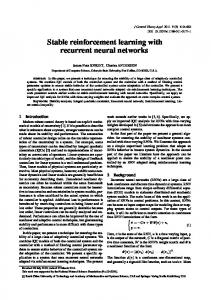
Table 1. Results of trained agents performing versus random-acting opponent agent

rew. soft

expl. starts -

hidden neurons h1 = 40 (one layer)

1

2

soft

-

h1 = 40, h2 = 20 (two layer)

3

soft

-

h1 = 120, h2 = 60 (two layer)

4

hard

X

h1 = 120, h2 = 60 (two layer)

3.1. Rewards Selectable there are two different kind of rewards given in a terminal state. A terminal state is defined as state where one of the two players has won. If the agent is not visiting this state in a certain time then the whole episode is restarted. Draw ending conditions are ignored as heuristic search algorithms would be required to detect them. One kind of rewards are hard rewards: ( 1 if agent has won hard reward = (3) 0 if agent has lost

winning-quota =

number of games won number of games lost

(5)

We have trained 4 different agents with varying learning parameters. However all agents have the following common parameters: • Initial weights between ±a, a = 0.4, Learning rate α continued falling over time on an inversed expfunction, α = 0.5, ..., 0.1

And then the soft reward based on the material balance: tanh( material )+1 6 2

500, 000 1, 000, 000 1, 500, 000 5, 000, 000 500, 000 1, 000, 000 1, 500, 000 5, 000, 000 500, 000 1, 000, 000 1, 500, 000 5, 000, 000 500, 000 1, 000, 000 1, 500, 000 5, 000, 000

win. quote 135 643 1, 050 515 305 665 310 700 424 2, 854 10, 000 infinity 1, 109 2, 498 3, 331 infinity

The results versus this opponent is given in a winningquota after 100, 000 tested episodes:

For the soft reward the material balance is calculated first: ( own: tokens + 1.5 ∗ kings if won material = opp: − (tokens + 1.5 ∗ kings) if lost

soft reward =

episodes

• Exploration rate  = 0.3, Discounting factor γ = 0.98, Training episodes: 5, 000, 000

(4)

Using the soft rewards the ending condition is therefore nonlinear credited by the material balance while the hard reward only evaluates the ending condition itself. Both reward methods have been tested and its results are given in the following section.

The results of the trained agents versus the randomacting opponent are listed in the table 1. Furthermore we have developed a software interface to Simple Draughts [7], which is a English Draughts computer program that uses a search tree calculated by Minimax and Alpha-Beta Pruning and can search up to a depth of 10. The results of our agents versus this computer program with varying search tree depths are listed in the table below. To assess the general performance of Simple Checkers we have also tested Simple Checkers versus the random-acting opponent and have observed that Simple Checkers on a search depth higher than 3 never looses. Afterwards we have performed tests manually between our intelligent agents and the draughts computer programs Chinook1 , CheckerBoard with the easych, simpletech and cake engine, NeuroDraughts2 and the

4. Results The intelligent agent has been trained by self-play, i.e. by interaction with an opponent that uses the same neural network for his move decisions. Both players had perfomed random moves at the same exploration rate  to avoid repeating episodes and to obtain balanced rewards. Another technique we have used optionally are exploring starts. At a random depth between 1 and 10, both players perform random moves resulting in a new starting position of the agent. The neural network is trained once per episode and after a certain amount of episodes the quality of the learned policy of the agent has been tested. To test the intelligent agent we have used an opponent that only performs moves randomly.

1 available at http://www.cs.ualberta.ca/ chinook/ ˜ play/ 1 available at http://www.fierz.ch/checkers.htm 2 available at http://iamlynch.com/nd.html

2927 2931 2919

cannot evaluate the differences between the agents that got the soft rewards and the hard rewards, as well as the usage of exploring starts. Our intuition is that the soft rewards are fitting better as the agent is more rewarded if he has more tokens than the opponent. For a novice human player agent 1 and 2 is hard to beat while agent 3 and 4 both seem to be unbeatable. However the real strength of agent 3 and 4 seems to be in the amateur league as they beat NeuroDraughts and Simple Checkers, both being amateur league players. We have introduced a gradient-descent TD algorithm that is neural approximated by a 4-layer MLP and have applied it to English Draughts. We have built multiple agents with different parameters and have compared them to a learning agent (NeuroDraughts) and various non-learning agents. Our best agent wins versus medium strong and looses to very strong computer players. Using this algorithm has helped our agent to reach an amateur league level.

Table 2. Results of trained agents performing versus Simple Draughts agent 1

2

3

4

episodes 500, 000 1, 000, 000 2, 000, 000 5, 000, 000 500, 000 1, 000, 000 3, 300, 000 5, 000, 000 500, 000 1, 000, 000 3, 200, 000 5, 000, 000 500, 000 1, 000, 000 2, 400, 000 5, 000, 000

won (depths) 1, 3 1−3 1, 3, 6 2, 3 4, 5 3, 7, 8 2 2 1, 2, 5, 6, 7 3 − 5, 9, 10 1, 2, 6 1, 5 2, 7 1 − 10 1

draw (depths) 8 3 7 6, 8, 9 3, 10 2 4 2, 7, 9, 10

relatively simple opponent KCheckers3 . Note that NeuroDraughts also is a learning agent while all other programs are non-learning agents. While agent 4 wins versus simpletech and NeuroDraughts, agent 3 wins versus easych, NeuroDraughts and KCheckers. All agents loose to Chinook and CheckerBoard with the strong cake engine.

References [1] Stuart J. Russel and Peter Norvig, Artificial Intelligence: A Modern Approach, 2nd Edition, Prentice Hall (2002).

5. Discussing the results and Conclusions

[2] Richard S. Sutton and Andrew G. Barto, Reinforcement Learning: An Introduction, MIT Press (Cambridge, MA, 1998).

Analyzing the results versus an random-action opponent, an agent performs better if he has experienced more training episodes and has more hidden neurons. However comparing these results to the ones obtained by playing versus Simple Draughts it is obvious that too much training episodes are worsening the performance. The ideal number of training episodes with the given continued decreasing learning rate seems to be between 2 − 3 millions. On the other hand the results with Simple Draughts are hard to interpret as it is possible for our agent to win on a higher search depth and to loose on a lower search depth. The simplest explanation is that there are plenty of good strategies in English Draughts and while being good in one situation does not implicite to be good in every game situation. Another interesting observation is that agent 3 and agent 4 plays the first move from 11 − 15 (named ’Old Faithful’) and agent 1 and agent 2 plays the first move from 9 − 14 (named ’Double Corner’) after the first 500, 000 training games. The ’Old Faithful’ is known as best and ’Double Corner’ as second best opening move. While all four agents change their strategies on further training episodes, they mostly start with the same first move. Although it was another objective of the research we 3 available

[3] Gerald Tesauro, Temporal Difference Learning and TD-Gammon, Communications of the ACM, Vol. 38, No. 3 (1995). [4] Jonathan Schaeffer, Neil Burch, Yngvi Bjoernsson, Akihiro Kishimoto, Martin Mueller, Robert Lake, Paul Lu, Steve Sutphen, Checkers Is Solved, Science Express Vol. 317. No 5488, pp. 1518 - 1522 (2007). [5] Christopher M. Bishop, Neural Networks for Pattern Recognition, Oxford University Press (1995). [6] G.V. Cybenko, Approximation by Superpositions of a Sigmoidal function, Mathematics of Control, Signals and Systems, vol. 2 pp. 303-314. electronic version (1989). [7] Nelson Castillo, Simple Draughts program, http://www.geocities.com/ ResearchTriangle/Thinktank/7379/ checkers.html (1999).

at http://qcheckers.sourceforge.net/

2928 2932 2920