Learning and Detecting Activities from Movement Trajectories Using the Hierarchical Hidden Markov Model Nam T. Nguyen, Dinh Q. Phung, Svetha Venkatesh Department of Computing Curtin University of Technology GPO Box U 1987, Perth, Western Australia {nguyentn,phungquo,svetha}@cs.curtin.edu.au Abstract Directly modeling the inherent hierarchy and shared structures of human behaviors, we present an application of the hierarchical hidden Markov model (HHMM) for the problem of activity recognition. We argue that to robustly model and recognize complex human activities, it is crucial to exploit both the natural hierarchical decomposition and shared semantics embedded in the movement trajectories. To this end, we propose the use of the HHMM, a rich stochastic model that has been recently extended to handle shared structures, for representing and recognizing a set of complex indoor activities. Furthermore, in the need of real-time recognition, we propose a Rao-Blackwellised particle filter (RBPF) that efficiently computes the filtering distribution at a constant time complexity for each new observation arrival. The main contributions of this paper lie in the application of the sharedstructure HHMM, the estimation of the model’s parameters at all levels simultaneously, and a construction of an RBPF approximate inference scheme. The experimental results in a real-world environment have confirmed our belief that directly modeling shared structures not only reduces computational cost, but also improves recognition accuracy when compared with the tree HHMM and the flat HMM.
1 Introduction Building intelligent systems in smart environments is the goal of much research [1, 6, 10, 11, 12, 13]. In most of these systems, modeling and recognizing activities, especially complex activities, is a crucial problem. Although activities can be inferred from a wide range of data given by sensors that pervade the environment, we restrict this discussion to data acquired through video cameras, that is, trajectories. When a person executes several actions in an environment, these actions can often be broken into smaller components. For example, the action of “making breakfast” involves a sequence of subtasks: (a) go to cupboard, (b) go to fridge, and (c) go to dining table. Another action, such as “cooking dinner”, may involve go to fridge, go to stove, and go to dining table. Thus, not only do normal activities have a natural hierarchy, they also have shared subactions.
Hung Bui Artificial Intelligence Center SRI International 333 Ravenswood Ave, Menlo Park CA 94025, USA,
[email protected]
The hidden Markov model (HMM) and some of its extensions, such as the couple hidden Markov model (CHMM) or the variable length Markov model (VLMM), are efficient for representing and recognizing simple activities [5, 9, 15]. However, these flat models are inadequate to model complex activities because they cannot characterize the hierarchic and shared structure naturally embedded in the activities. Earlier approaches to tackling this problem include the layered hidden Markov model (LHMM) [14], stochastic context free grammar (SCFG) [17], the abstract hidden Markov model (AHMM) [4], and the hierarchical hidden Markov model (HHMM) [8, 3]. In [14], Oliver et al. use the LHMM for recognizing highlevel activities based on real-time streams of signals from multiple sources of sensors. The activities are classified level by level using the HMM. The inference influence in the activity hierarchy is one way: from low level to high level. Ivanov and Bobick [11] propose a two-stage algorithm for behavior recognition. The primitive behaviors are detected at low level using the basic HMM. Then, the system uses an SCFG to recognize high-level behaviors. These approaches, however, do not offer an integrated method for inferring behaviors all the way from low level to high level. A fully integrated system for modeling and detecting both high-level and low-level behaviors is proposed by Nguyen et al. [13]. The system uses the abstract hidden Markov memory model (AHMEM) [2] to model the behavior hierarchy. Although the system is expressive in representing high-level behaviors, it is limited in learning the behaviors’ parameters. Osentoski et al. [16] introduce a system using the AHMM [4] for representing the behaviors. Parameters for the model can be learned from labeled or unlabeled data using the expectation maximization (EM) algorithm, in which the inference at the E-step is achieved by the junction tree algorithm. However, when the depth of the model increases, this method can quickly become intractable because of the blow up in the maximum clique size. Another limitation of this system is that special landmarks are not taken into account, thus limiting the expressiveness of the behavior hierarchy. Liao et al. [12] propose a surveillance system using GPS sensors to infer a user’s daily activities in a large and complex environment. The AHMM is used to represent the activity hierarchy, which has the following levels: (1) user’s goals, (2)
trip segments (start locations, stop locations, and modes of transportation), and (3) user’s locations and velocities. The EM algorithm is used to learn the user’s goals and important locations from unlabeled data. The parameters of the hierarchical activity are then estimated using the Monte Carlo EM method [19]. It is not clear how the accuracy of this method would degrade when the complexity of the model and the observation length increase. This paper aims to use the HHMM, in particular its recent extension [3] that allows for shared structures, for tackling two issues: (a) modeling and learning complex behaviors from human indoor trajectories and (b) recognizing the behaviors from new trajectories. We argue that to build robust and scalable behavior recognition systems, it is crucial to model not only the natural hierarchical decomposition in the movement trajectories, but also the inherent shared structure embedded in the hierarchy. The shared structures can also be duplicated and represented using a tree-like structure as in [8], but as empirically shown in this paper, our proposed shared structure model not only saves computational time but is also superior in the recognition accuracy when compared against the tree HHMM and the flat HHM. In addition, using the HHMM to model activities allows us to incorporate prior knowledge about the structure of the behavioral hierarchy. In the need of real-time inference, the Rao-Blackwellised particle filter (RBPF) used in the dynamic Bayesian network (DBN) [7] and especially in the AHMM [4] is adapted to provide an efficient approximate inference method. Empirical results demonstrating the advantages of this RBPF scheme over the exact inference method are also reported. The novelty of this paper is threefold. (1) To the best of our knowledge, we are the first to apply the HHMM with shared structures to the problem of activity recognition in a real environment and we demonstrate its superiority over the flat HMM and tree HHMM. (2) We estimate the model parameters in an integrated way, as compared with other approaches that employ level-by-level parameter estimation [14, 11]. Our learning framework goes beyond the work of Osentoski et al. [16] and Liao et al. [12] by using an efficient, scalable, and exact algorithm for the problem of learning the model’s parameters, as opposed to the use of the EM and junction tree inference algorithms in [16] or the Monte Carlo EM algorithm in [12]. (3) We adapt the RBPF algorithm to the HHMM and compare the results with an exact inference algorithm, demonstrating the usefulness of this approximate inference scheme.
2 Hierarchical Hidden Markov Models The HHMM, first introduced in [8], extends the traditional HMM [18] in a hierarchic manner to include a hierarchy of hidden states. Each state in the normal HMM is generalized recursively as another sub-HMM with special end states included to signal when the control of the activation is returned to the parent HMM. The original HHMM in [8], however, requires a strict tree-like structure in the topological specification and thus limits its expressiveness and hinders its applications. This problem has been tackled recently in [3], in which a generalized form of the HHMM is introduced whose
topology can be a general lattice structure. More important, the extended HHMM can model shared structures that naturally exist in the domain. Because of the space restriction, we outline this model in the next section and refer readers to [3] for further details.
2.1 HHMM: Model definition A discrete HHMM is formally defined by a 3-tuple < ζ, Y, θ >: a topological structure ζ, an observation alphabet Y, and a set of parameters θ. The topology ζ specifies the number of levels D, the state space at each level, and the parent-children relationship between levels d and d + 1. The states at the lowest level (level D) are called production states. The states at a higher level d < D are termed abstract states. Only production states emit observation. Given a topological specification ζ and the observation space Y, the set of parameters θ is defined as follows. Denote By|p as the probability of observing y ∈ Y given that the production state is p. For each abstract state p∗ at level d and the set of its chil∗ dren ch(p∗ ), we denote π d,p as the initial distribution over ∗ ch(p∗ ), Ad,p i,j as the transition probability from child i to child ∗ j (i, j ∈ ch(p∗ )), and Ad,p i,end as the probability that p terminates given its current child is i. The set of parameters θ is ∗ ∗ d,p∗ ∗ {By|p , π d,p , Ad,p i,j , Ai,end | ∀(y, p, d, p , i, j)}. An abstract state p∗ at level d can be executed as follows. First, p∗ selects a state i at the lower level d + 1 from the ini∗ tial distribution π d,p . Then, i is executed until it terminates. ∗ ∗ At this time, p∗ can terminate with probability Ad,p i,end . If p does not terminate, it continues to select a state j for execu∗ ∗ tion from the distribution Ad,p i,j . The loop continues until p terminates. The execution of p∗ is similar to the execution of an abstract policy π ∗ in the AHMM [4], except that π ∗ selects a lower level policy π based only on the state at the bottom level, not on the policy π 0 selected in the previous step. However, the abstract state is a special case of the abstract policy in the AHMEM [2] (an extension of the AHMM). A representation of the HHMM as a DBN is provided in [3], which defines a joint probability distribution (JPD) over the set of all variables {xdt , edt , yt | ∀(t, d)}, where xdt is the state at level d and time t, edt represents whether xdt terminates or not, and yt is the observation at time t. ∗
2.2 Learning parameters in the HHMM We need to learn the set of parameters θ of the HHMM from an observation sequence O. Bui et al. [3] have proposed a method based on the EM algorithm and the asymmetric inside-outside (AIO) algorithm to estimate θ. For this method, the set of hidden variables is H = {xdt , edt |t = 1, . . . , T, d = 1, . . . , D}, where T is the length of the observation sequence. The set of observed variables is O = {y1 , . . . , yT }. Assume that τ is the sufficient statistic for θ. The EM algorithm reestimates θ by first calculating the expected sufficient statistic (ESS) τ¯ = EH|O τ . Then, the result is normalized to obtain the new value P for θ. The∗ ESS t=T −1 d,p ξt (i,j) d,p∗ for the parameter Ai,j , for example, is t=1 Pr(O) ,
d = i, xd+1 where ξtd,p (i, j) = Pr(xdt = p∗ , xd+1 t t+1 = j, et = ∗ d,p F, etd+1 = T, O). The ESS for Ai,j can be computed by the AIO algorithm [3]. The ESS for the other parameters of θ is computed in a similar manner. The complexity for the AIO algorithm is cubic in the length of the observation sequence, but linear in the number of states of the model. ∗
2.3 Exact and approximate inference for the HHMM The AIO algorithm can be used directly to derive an exd,p∗ act filtering algorithm as follows. At time t, ξt−1 (i, j) d,p∗ is computed by the AIO algorithm. Summing ξt−1 (i, j) over p∗ , i, edt−1 and ed+1 t−1 , we obtain the probability ∗ d+1 Pr(xt |y1 , . . . , yt ). Note that, at the next time, ξtd,p (i, j) ∗ d,p can be derived from ξt−1 (i, j) by stretching this probability one more time slice. Thus, the complexity of the exact filtering algorithm is O(T 2 ). This algorithm can be well suited for short-term recognition, but it might not be realistic for a real-time recognition task when the observation length T grows. Alternatively, the RBPF has been successfully deployed in the AHMM [2] and can be readily adapted for the HHMM. Denote: x1:D , {x1t , . . . , xD t t }, 1:D 1 D 1:D 1:D et , {et , . . . , et }, e1:t , {e1 , . . . , e1:D }, y , 1:t t {y1 , . . . , yt }. The idea of the RBPF is that the filtering dis1:D tribution at time t − that is, Pr(x1:D | y1:t ) − is apt , et proximated via a two-step procedure: (1) sampling the RaoBlackwellised (RB) variable e1:D from the current RB belief t 1:D state Bt = Pr(x1:D , e1:D t t , yt | e1:t−1 ), and (2) updating the RB belief state Bt using exact inference. At each time step t, the algorithm maintains a set of N samples, each consisting of the distribution of one slice network Ct , Pr(x1:D | e1:D t 1:t−1 ). The RB belief state Bt can be obtained directly from Ct by adding in the network representing the conditional distribution of yt and e1:D t . A new sample e1:D can be obtained from the canonical form of Ct (after obt sorbing yt ). At the next time slice, Ct+1 is constructed by projecting Ct over one slice based on the sampled value of e1:D t . The complete algorithm is shown in Algorithm 1. The complexity of the RBPF algorithm for the HHMM is O(N D), where N is the number of samples and D is the depth of the model.
3 Implementation We apply the HHMM with shared structure to model people behaviors in a real environment. The environment is a room in which two static cameras are used to track people. We are interested in some special landmarks in the environment: the stove, cupboard, dining chair, fridge, TV chair, and door. Fig. 1(a) and (b) show the room and the special landmarks viewed from the two cameras. The room is divided into a grid of cells or states, which are numbered 1, 2,. . . , 24 (Fig. 2). A two-level behavior hierarchy is defined in the environment. The top level consists of complex behaviors and the
Algorithm 1 RBPF for the HHMM Begin For t = 1, 2, . . . /* sampling step */ For each sample i = 1, 2, . . . , N (i) Absorb yt into Ct (i) (i) Canonicalize Ct , update weight wt = Bt (yt ) 1:D(i) (i) Sample et from Ct and Pr(e1:D | x1:D t ) t /* re-sampling step */ (i) Normalize the weight w ˜ (i) = PNw w(i) i=1
End
Re-sample the sample set according to w ˜ (i) /* exact step */ For each sample i = 1, 2, . . . , N (i) (i) 1:D(i) Compute Ct+1 from Ct and et /* Estimation step */ PN (i) d Compute Pr(xdt+1 | y1:t ) ≈ N1 i=1 Ct+1 (xt+1 )
Door
TV chair
Fridge
Dining chair
(a) camera 1
Stove
Cupboard Dining chair
Fridge
TV chair
(b) camera 2
Figure 1. The scene viewed from the two cameras.
bottom level consists of primitive behaviors. A primitive behavior is a person’s action of going from one landmark to another. The primitive behavior terminates when the person reaches the designated landmark. Table 1 shows 12 primitive behaviors defined in the environment. A complex behavior is a person’s action of visiting a sequence of landmarks. It can be refined into a sequence of primitive behaviors. We consider three complex behaviors − short meal, have snack, and normal meal − of which the topologies are shown in Fig. 3(a), (b), and (c), respectively. Note that the topologies of these complex behaviors are specified by observing their typical patterns in the environment. A person executing behavior short meal will first enter the room via the door, go to the cupboard, and go to the fridge. Then, the person may exit the room via the door or go to the dining chair. From the dining chair, the person can exit the room or come back to the fridge. In the latter case, he again has two choices: exiting the room or going to the dining chair (Fig. 3(a)). The behavior short meal involves the following landmarks: the door, cupboard, fridge, and dining chair. This complex behavior can be refined into a sequence of primitive
Cupboard
Start
Camera 1
Door
Stove
Fridge
TV chair
1
2
3
4
5
6
7
8
beh 1 Cupboard
Start Start
Dining chair
9
10
11
12
13
14
15
16
17
18
19
20
21
22
23
24
Door
beh 8
Cupboard
Fridge
Dining chair
Dining chair
beh 12
beh 12 Fridge
beh 7
Door
Landmarks Fridge→TV chair TV chair→Door Fridge→Stove Stove→Dining chair Fridge→Door Dining chair→Fridge
Table 1. The set of primitive behaviors.
behaviors 1, 2, 3, 4, 11, and 12. The primitive and complex behaviors are mapped into a shared-structure HHMM, which has four levels. Level 1 is a root behavior. Levels 2 and 3 are the complex and primitive behaviors, respectively. Level 4 represents the states of the environment. Observations of these states are the cells in the environment. The hierarchy of behaviors and states is shown in Fig. 4. Note that some primitive behaviors are shared by multiple complex behaviors; for example, behavior 2 is shared by short meal, have snack, and normal meal. The parameters of the HHMM are the matrices π d,p , Ad,p , Ad,p [end] , and the observation model B, where d = 1, 2, or 3 and p is a behavior at level d.
4 Experimental Results 4.1 Data and evaluations The training data consists of 45 observation sequences obtained from 45 real scenarios. In each scenario, a person executes one of the three complex behaviors: short meal, have snack, and normal meal. The person’s trajectory is obtained from the tracking system, and converted into a sequence of cells or observations. As a result, we have 45 observation sequences. The test data is a different set of 43 observation sequences obtained in a similar way. We evaluate the performance of different models in behavior recognition based on the accuracy rate, early detection, and correct duration. First, the winning behavior of an ob-
Door
Terminate
Terminate
(a) short meal
beh 9
beh 11
beh 4
Figure 2. The environment used in the system.
Landmarks Beh. Door→Cupboard 7 Cupboard→Fridge 8 Fridge→Dining chair 9 Dining chair→Door 10 Door→TV chair 11 TV chair→Cupboard 12
beh 10 beh 4
beh 2 Fridge
Door
Beh. 1 2 3 4 5 6
Stove
Cupboard
beh 3
Door
beh 9
TV chair beh 6
beh 2
Camera 2
Fridge
beh 5
beh 1
beh 11
beh 2
Door
(b) have snack
Terminate
(c) normal meal
Figure 3. The complex behaviors. Level 1 Root behavior Level 2 Short_meal
Have_snack
Normal_meal
Behavior 1 Behavior 2 Behavior 3 Behavior 4 Behavior 11 Behavior 12
Behavior 2 Behavior 5 Behavior 6 Behavior 7 Behavior 8
Behavior 1 Behavior 2 Behavior 4 Behavior 9 Behavior 10 Behavior 11 Behavior 12
Level 3
Level 4 States 1,2,...,24
Figure 4. The behavior and state hierarchy.
servation sequence is defined as the complex behavior that is assigned the highest probability at the end of the sequence. Then, the accuracy rate is the ratio of the number of observation sequences, of which the winning behavior matches the ground truth, to the total number of test sequences. When the winning behavior matches the ground truth, we define: ∗ early detection , tT , where T is the observation sequence length, and t∗ = min{t| Pr(winning behavior) is highest from time t to T }. The early detection represents how early the system detects the winning behavior. We define: correct duration , PT , where P is the total of the time period, in which the primitive behavior assigned the highest probability matches the ground truth. Note that the early detection and the correct duration refer to recognition performance at different levels in the hierarchy; they do not necessarily sum up to more (or less) than 100%. A reliable system in behavior recognition will have high accuracy rate, low early detection, and high correct duration.
Learned HHMM
4.2 Performance of hand-coded HHMM The parameters of the hand-coded HHMM are initialized by observing typical patterns of the three complex behaviors short meal, have snack, and normal meal. The exact filtering algorithm is used with the hand-coded HHMM to infer the behaviors at different levels. Fig. 5(a) shows the probability distribution of the complex behaviors for an observation sequence over time. From time t∗ = 25 to the end of the sequence, normal meal is being assigned the highest probability. Thus, normal meal is the winning behavior of this sequence and the early detection is t∗ /T = 25/52 ≈ 48.08%. We consider the results of querying the primitive behavior. The ground truth for this observation sequence is that a person executes primitive behaviors 1, 2, 9, 10, and 4 consecutively, with the corresponding starting times 1, 13, 25, 27, and 36, respectively. Fig. 5(b) shows the probabilities that the system assigns the primitive behaviors over time (behaviors with insignificant probability are omitted from the figure). The correct duration is approximately 94.23%, meaning that most of time the system detects the primitive behavior correctly. 1.2
Probability
1.2
short_meal have_snack normal_meal
1 0.8
0.8
0.6
0.6
0.4
0.4
0.2
0.2
0
10
20 t*=25 30 Time
40
(a) Complex behavior
beh 1 beh 2 beh 3 beh 4 beh 5 beh 9 beh 10
1
T=52
0
12
24 27
35
T=52
Time
(b) Primitive behavior
Figure 5. Querying the behaviors with the hand-coded HHMM.
Considering the results of querying the behaviors in the test data, which consists of 43 test sequences, the system recognizes correctly the winning behavior in 41 sequences. The accuracy rate is 41/43 ≈ 95.35%. The averages of the early detection and correct duration are 52.90% and 66.72%, respectively.
4.3 Comparing learned HHMM with hand-coded HHMM, flat HMM, and tree HHMM Compare against hand-coded HHMM. We learn the parameters of the HHMM using the EM and AIO algorithms [3] to obtain the learned HHMM. The training data is provided in Section 4.1. The learned HHMM is then used to recognize the behaviors in the 43 test sequences. Table 2 shows the performance of the learned HHMM in comparison with the hand-coded HHMM. The accuracy rate of the learned HHMM is higher than that of the hand-coded HHMM (100% versus 95.35%). The early detection of the learned HHMM is lower than that of the hand-coded HHMM (16.96% versus 52.90%), meaning that the learned HHMM is able to detect the winning behavior earlier. The correct duration of the learned HHMM is also higher than that of the hand-coded HHMM. The results show that the learned HHMM outperforms the hand-coded HHMM in behavior recognition.
Accuracy rate 100% Early detection 16.96% Correct duration 73.44%
Handcoded HHMM 95.35% 52.90% 66.72%
Flat HMMs
Tree HHMM
90.70% 27.96%
100% 31.74% 49.21%
Table 2. Performance of the learned HHMM, hand-coded HHMM, flat HMM and tree HHMM.
Compare against flat HMM. We use the flat HMM to recognize complex behavior. An HMM is created for each complex behavior short meal, have snack, or normal meal. The parameters of an HMM are learned using the training data in Section 4.1. Table 2 compares the performance of the flat HMM with the learned HHMM. The same test data in Section 4.1 is used to evaluate the two models. The accuracy rate of the system with the flat HMM is lower than that of the system with the learned HHMM (90.70% versus 100%). The average of the early detection of the system with the flat HMM is 27.96%, which is higher than that of the system with the learned HHMM (16.96%). The results show that the learned HHMM is able to recognize the complex behaviors more accurately and earlier than the flat HMM. Compare against tree HHMM. We create a tree HHMM from the shared-structure HHMM defined in Section 3 by duplicating each primitive behavior being the child of two complex behaviors (Fig. 6). The parameters for the tree HHMM are estimated using the EM algorithm with the training data provided in Section 4.1. The averaged time per one iteration in the case of the tree HHMM is about 1.5 times slower than that of the shared-structure HHMM. We use the tree HHMM to recognize behaviors in the 43 test sequences. The results in Table 2 show that the shared-structure HHMM recognizes the behaviors more reliably than the tree HHMM. Short_meal Behavior 1 Behavior 2 Behavior 3 Behavior 4 Behavior 11 Behavior 12
Behavior 1 = Behavior 14 Behavior 4 = Behavior 16 Behavior 12 = Behavior 18
Have_snack Behavior 13 Behavior 5 Behavior 6 Behavior 7 Behavior 8
Normal_meal Behavior 14 Behavior 15 Behavior 16 Behavior 9 Behavior 10 Behavior 17 Behavior 18
Behavior 2 = Behavior 13 = Behavior 15 Behavior 11 = Behavior 17
Figure 6. The primitive and complex behaviors of the tree HHMM.
4.4 Comparing the exact filtering algorithm with the RBPF So far in this section, we have used the exact filtering algorithm based on the AIO method for behavior recognition. The computational complexity of this algorithm is O(T 2 ). Thus, it is not realistic in long scenarios. Alternatively, we can use
the RBPF as discussed in Section 2 for the inference task. Table 3 compares the results of querying the behaviors using the RBPF and exact filtering algorithm. The test data described in Section 4.1 is used. When the number of samples N = 50, the RBPF misclassifies the complex behavor in a test observation sequence. The accuracy rate is 42/43 ≈ 97.67%. But when N = 200, the RBPF detects correctly the complex behaviors in all test sequences (the accuracy rate is 100%). The early detection and correct duration obtained by the RBPF are about the same as the results obtained by the exact filtering algorithm (Table 3). Fig. 7 compares the running time of the RBPF with the exact filtering algorithm. The running time for each time t of the RBPF is nearly constant, while that of the exact filtering algorithm increases significantly when t increases. As in the figure, when N = 50 and 200, the running time of the RBPF is less than that of the exact filtering algorithm from time t1 = 3 and t2 = 10, respectively. At the end of the observation sequence (t=52), the RBPF is much faster than the exact filtering algorithm. Exact filtering Accuracy rate Early detection Correct duration
100% 16.96% 73.44%
RBPF N = 50 N = 200 97.67% 100% 14.74% 15.97% 73.45% 72.88%
Table 3. Comparing the performance of the exact filtering algorithm with the RBPF algorithm. 7
Exact filtering RBPF (N=50) RBPF (N=200)
6
Time (seconds)
5 4 3 2 1 0
t1=3
t2=10
20
30
40
T=52
Figure 7. The running time for each time stamp of the exact inference and RBPF algorithms.
5 Conclusion We have presented the use of the shared-structure HHMM to recognize people behaviors. The parameters of the HHMM have been learned from real and unlabeled data. We have used both the exact approximate inference algorithm and the RBPF to infer behaviors at different levels. Experimental results in a real environment demonstrate the ability of the sharedstructure HHMM to track people behaviors reliably, and the superiority of the shared-structure HHMM over the flat HMM and tree HHMM. The results also show the advantages of the RBPF inference algorithm to an exact method in a real application.
Acknowledgement
Hung Bui is supported by the Defense Advanced Research Projects Agency (DARPA), through the Department of the Interior, NBC, Acquisition Services Division, under Contract No. NBCHD030010.
References [1] D. Ayers and M. Shah. Monitoring human behavior from video taken in an office environment. Image and Vision Computing, 19(12):833–846, October 2001. [2] H. H. Bui. A general model for online probabilistic plan recognition. In Proceedings of the Eighteenth International Joint Conference on Artificial Intelligence (IJCAI-03), 2003. [3] H. H. Bui, D. Q. Phung, and S. Venkatesh. Hierarchical hidden Markov models with general state hierarchy. In Proceedings of the Nineteenth National Conference on Artificial Intelligence, pages 324–329, San Jose, California, 2004. [4] H. H. Bui, S. Venkatesh, and G. West. Policy recognition in the abstract hidden Markov model. Journal of Artficial Intelligence Research, 17:451–499, 2002. [5] G. Cielniak, M. Bennewitz, and W. Burgard. Where is ...? Learning and utilizing motion patterns of persons with mobile robots. In Eighteenth International Joint Conference on Artificial Intelligence (IJCAI), pages 909–914, Acapulco, Mexico, August 2003. [6] R. Collins, A. Lipton, T. Kanade, H. Fujiyoshi, D. Duggins, Y. Tsin, D. Tolliver, N. Enomoto, and O. Hasegawa. A System for Video Surveillance and Monitoring. Technical Report CMU-RI-TR-00-12, Robotics Institute, Carnegie Mellon University, May 2000. [7] A. Doucet, N. de Freitas, K. Murphy, and S. Russell. RaoBlackwellised particle filtering for dynamic Bayesian networks. In Proceedings of the Sixteenth Annual Conference on Uncertainty in Artificial Intelligence, 2000. [8] S. Fine, Y. Singer, and N. Tishby. The hierarchical hidden Markov model: Analysis and applications. Machine Learning, 32(1):41–62, 1998. [9] A. Galata, N. Johnson, and D. Hogg. Learning variable length Markov models of behaviour. Computer Vision and Image Understanding Journal, 81:398–413, 2001. [10] E. Grimson. VSAM. URL: http://www.ai.mit.edu/projects/darpa/vsam, 1998. [11] Y. Ivanov and A. Bobick. Recognition of visual activities and interactions by stochastic parsing. IEEE Transactions on Pattern Recognition and Machine Intelligence, 22(8):852–872, August 2000. [12] L. Liao, D. Fox, and H. Kautz. Learning and inferring transportation routines. Proceedings of the National Conference on Artificial Intelligence(AAAI-04), 2004. [13] N. T. Nguyen, H. H. Bui, S. Venkatesh, and G. West. Recognising and monitoring high-level behaviours in complex spatial environments. In IEEE Conference on Computer Vision and Pattern Recognition, 2003. [14] N. Oliver, E. Horvitz, and A. Garg. Layered representations for human activity recognition. In Fourth IEEE International Conference on Multimodal Interfaces, pages 3–8, October 2002. [15] N. M. Oliver, B. Rosario, and A. Pentland. A Bayesian computer vision system for modeling human interactions. IEEE Transactions on Pattern Analysis and Machine Intelligence, 22(8):831–843, 2000. [16] S. Osentoski, V. Manfredi, and S. Mahadevan. Learning hierarchical models of activity. IEEE/RSJ International Conference on Robots and Systems (IROS), to appear, 2004. [17] D. V. Pynadath and M. P. Wellman. Generalized queries on probabilistic context-free grammars. IEEE Transactions on Pattern Analysis and Machine Intelligence, 20(1):65–77, 1998. [18] L. R. Rabiner. A tutorial on hidden Markov models and selected applications in speech recognition. Proceedings of the IEEE, 77(2):257–286, February 1989. [19] G. Wei and M. Tanner. A Monte-Carlo implementation of the EM algorithm and the poor man’s data augmentation algorithms. Journal of the American Statistical Association, 85:699–704, 1990.