Learning-Assisted Evolutionary Search for Scalable Function Optimization: LEM(ID3) Guleng Sheri, Member, IEEE and David Corne, Member, IEEE
Abstract— Inspired originally by the Learnable Evolution Model(LEM) [5], we investigate LEM(ID3), a hybrid of evolutionary search with ID3 decision tree learning. LEM(ID3) involves interleaved periods of learning and evolution, adopting the decision tree construction algorithm ID3 as the learning method, and a steady state EA as the evolution component. In the learning periods, ID3 is used to infer rules that attempt to identify ‘good’ regions for genes, based on the values of one or more other genes. The rules are then used to guide the generation of new individuals. Without any preliminary parameter tuning, we evaluate LEM(ID3) on the test suite of 25 functions designed the CEC 2005 special session on Real-Parameter Optimization. We describe the results, and in particular compare with the three most successful algorithms from the CEC 2005 competition; Sinha et al’s K-PCX, and two versions of Auger and Hansen’s CMA-ES. We find that LEM(ID3)’s performance is competitive with these algorithms, increasingly so as the problem dimensionality increases. In the case of 50-Dimensions, LEM(ID3) clearly records better overall performance on this function suite than the three comparative algorithms. Research-strength LEM(ID3) code is freely available at http://www.macs.hw.ac.uk/ gls3/LEMID3/LEMID3.zip .
I. I NTRODUCTION The Learnable Evolution Model (LEM, [5]) was introduced in 2000, as a highly generalised hybrid approach to optimisation, in which the overall idea is to run repeated phases of evolution and learning in series. Each ‘evolution’ period is informed in some way by the previous ‘learning’ period. In the learning periods, the general idea is to use a machine learning technique to infer relationships between gene values and fitness. For example, we may start by running an evolutionary algorithm for 10 generations; then we halt the evolutionary algorithm and do some learning (perhaps a neural network, or an AQ rule learner – as in the original LEM – and so on). The result of the learning phase is then used in the next period of evolution. The way in which learning influences evolution is not restricted by (our view of) the LEM framework. E.g. the learned model could be used to predict the fitness (or fitness category) of children before they are evaluated, and the evolution phase discards, without evaluation, children that are predicted to be particularly unfit. Or, the learned model may be used to constrain genetic operators in a beneficial way. Or, the learned model may be used to ‘repair’ children that are Guleng Sheri is with the Department of Computer Science, Heriot-Watt University, Edinburgh, Scotland, UK. (phone: +44 (0)131 4514197; email:
[email protected] ). David Corne is with the Department of Computer Science, Heriot-Watt University, Edinburgh, Scotland, UK. (phone: +44 (0)131 4513410; email:
[email protected]).
otherwise generated by standard operators. Evolution then continues for another few generations, resulting in new data for the learning method (chromosomes and their evaluated fitnesses), and so it continues. The learning method in most LEM work [5] is AQ15 [14], and the reported results tend to be very promising, with improvements in solution quality and dramatic speedup when compared to the ‘without learnig’ equivalent EA. In application-oriented work, a multiobjective LEM-based approach, using C4.5 [8] as the learning method, was found to significantly speed up and improve solution quality for large-scale problems in water distribution networks [3]. The developers of the LEM framework are continually updating the ”AQ15” version [15] and continue to report impressive results, albeit on a limited suite of test functions. Meanwhile, of course, Estimation of Distribution Algorithms (EDAs) [4] can also be viewed as learning/evolution hybrids, with the emphasis on building and maintaining models of fit chromosomes. While EDAs focus on modelling (i.e. search is guided closely by statistical models, with new sample points generated directly from the model), in LEM the evolutionary component is responsible for the search (i.e. new points are sampled mainly in the usual way by using genetic operators), with guidance from learning. Recent results using LEM3 compare EDAs and LEM3 [16], and report better quality results than a good EDA on two hard functions, with between 15 and 230 fold speedup of LEM3 over the EDA. Also, of couse, hybrids of EDA and GAs (e.g. [6], [13]) are also successful optimisers. LEM is similar in style to a hybrid of EDA and EA. The design and application of LEM is clearly worth considerably more research. The speedup reported in several papers that apply LEM – that is, the reduction in the number of fitness evaluations needed to reach high quality results, is of particular interest for many important applications in which fitness evaluation is costly. In some applications, such time savings can make the difference between the problem being solvable at all or not. With an interest in clearer understanding of the LEM framework and its performance, we investigated in [9] the improvements obtainable by using perhaps the simplest possible learning method within the LEM frameork - namely k-nearest neighbour learning. In LEM(KNN), the learning phase comprised only the process of identifying the best and worst 30% of the current population; subsequent evolution only allowed evaluation of children for whom the majority of their 5 nearest neighbours from these sets were in the higher-fitness group. Although not able to produce results that rivalled those of Michalski’s
published LEM results, this simple intervention of learning provided very significant speedup and solution quality improvements over the unchanged EA. In [10] we investigated another simple learning scheme within LEM, which we called entropy-based discretization. The learning process in this case was to infer a good and a bad interval for each parameter in the search based, by finding a partition of that parameter’s range that had optimal entropy. Subsequent mutations for any given parameter were then confined to be within the most recenyly learned good intervals. We found that LEM(ED) again provided significant advantages in both solution speed and quality over the unchanged EA, and on most problems (although only a small suite of 7 problems was studied) it was also superior to CMA-ES when the number of evaluations was limited, and was significantly better than LEM(KNN). In this paper, we explore a new variant in which the learning method used is the ID3 decision tree learner [7]. Based on chromosome data and evaluated fitnesses, ID3 is used to repeatedly find rules that predict, on the basis of subsets of the genes, whether a chromosome is good or not. We would expect this new approach to be capable of better results than LEM(ED), largely because the learned rules are able to navigate interactions between any number of parameters. In the remainder we continue as follows. Section 2 provides more detail on the original LEM and on LEM(ID3). Section 3 then details our experiments, and results, section 4 gives a concluding discussion. II. LEM
AND
LEM(ID3)
A. LEM(AQ) and the LEM framework In LEM(AQ), an initial population is divided into high-performance (H-group) and low-performance (L-group) groups according to fitness; these two groups are stored as positive and negative training examples for AQ learning algorithm. The outcome of learning is a set of rules which predict a class label (i.e. H-group or L-group). LEM(AQ) then proceeds with an otherwise normal EA, except that the operators generate new individuals only with gene values within the ranges sanctioned by the recently learned rules. LEM(AQ) then continues for a specific amount of generations, and then pauses for more learning based on the current population. This feeds into the next stage of evolution, and so on. LEM(AQ) has many additional details that mediate the transitions between learning and evolution, and we refer readers to [5] for more details. LEM(AQ) is one instantiation of the wider LEM framework, which allows for creativity in the choices of learning method, and the way in which learning and evolution interact. In this paper, we continue to investigate the LEM framework, and focus on an approach in which the learning mechanism is ID3. B. The LEM(ID3) algorithm We assume readers are familiar with the ID3 decision tree learning algorithm [7]. We note only that standard ID3
requires discrete, nominal data (rather than real values), and within LEM(ID3) it is always treats a real-valued range as a set of discrete equal-width intervals. As we will see, this is initially set to 2 intervals for each gene, but adapts during the search. In LEM(ID3), ID3 is employed to learn from a population of evaluated chromosomes. Each chromosome is labelled as either high-performance or low-performance (see below), and ID3 learns a tree that predicts this label from the gene values. Further details are given next. LEM(ID3) contains two main components: evolution and learning. In the evolution component, a standard evolutionary algorithm is applied. In the learning component, ID3 is used, in a way detailed below. LEM(ID3) divides the current population into a highperformance (H-group) and low-performance (L-group) groups according to their fitness values and a given threshold (say, 30% - that is, the fittest 30% form the H-group and the worst 30% form the L-group). ID3 then uses the H-group and L-group as the training data to construct the decision tree, which is then transformed into a set of rules. These sets of rules are the hypotheses that differentiates between the two groups. New individuals are generated by instantiating these hypotheses, or by evolution, or are randomly generated. The learning mode continues until there is no better individual generated for a certain number of generations, or the diversity of the population is too small. The evolution mode begins when the learning mode is finished, offering the opportunity to escape from local optima and also preserve diversity, which is crucial for success in the subsequent learning phase. Evolution continues for a certain number of generations, before the learning phase begins again. The overall pseudo-code of LEM(ID3) is set out here as Algorithm 1, with some components elaborated further later in the paper. 1) The Learning Mode: In the learning mode, there are three main steps. First, select training examples. Second, learn and generate hypotheses. Third, instantiate hypotheses and generate new individuals. •
•
To select the training examples, we use ‘populationbased selection’ ([5]), in which we specify that a given percentage of the population will be in the H-group and a given pecentage will be in the L-group. We use 30% in both cases – i.e., after sorting the individuals by fitness value, the top 30% are placed into the Hgroup and the lowest 30% are put in the L-group. An alternative discussed in [5], but which is more problematic to implement, is based on speifying fitness value thresholds. Learn and generate hypotheses: Given the training examples, in LEM(ID3) we use ID3 to construct a decision tree. The construction procedure is straightforward, as discussed above. The resulting tree can be transformed into a set of rules, which can then be seen as hypotheses discriminating H-group and L-group individuals. An example decision tree produced during a LEM(ID3) run is given in Figure 1.
Algorithm 1 pseudo code for LEM(ID3) 1: Generate initial population and evaluate each chromosome. 2: repeat 3: while Termination condition for learning is not satisfied do 4: Form the H-group and L-group from the current population. 5: Using the H-group and L-group, learn a decision tree and transform it into a set of rules. 6: Generate some new individuals for the next generation by instantiating new chromosomes guided by the learned rules. 7: Generate some new individuals for the next generation by evolution (mutation and crossover ) or at random. 8: end while 9: while Termination condition for evolution is not satisfied do 10: operate a standard evolutionary algorithm. 11: end while 12: adjust discretization. 13: until Termination condition for LEM(ID3) is satisfied Attri7
( −0.2 ... 0.3 )
(1.4 ... 2.3 ) (0.3 ... 1.4 ) Attri9
Attri12 Attri4 ( 3.0 ... 5.2 )
(−5.0 ... −4.1 ) ( −1.0 ... −2.2 )
Attri3
Low
Low High
Attri26
Low (7.0 ... 9.0 )
( −7.0 ... 0.0 )
High Low
Fig. 1.
Low
High
a learned decision tree and it’s expression for H-group
The ruleset produced from the decision tree in Figure 1 is as follows. attri7 == (−0.2 . . . 0.3) ∧ attri12 == (3.0 . . . 5.2)∧ attri3 == (−7.0 . . . 0.0) =⇒ H
attri7 == (0.3 . . . 1.4) ∧ attri4 == (−1.0 · · · − 2.2)∧ =⇒ H
attri7 == (1.4 . . . 2.3) ∧ attri9 == (−5.0 · · · − 4.1)∧
attri26 == (7.0 . . . 9.0) =⇒ H
•
where each rule expresses a path rooted from attri7 to leaf nodes H, the classification. For example, the path attri7 , attri12 , and attri3 is a path in the decision tree constructed by ID3, and any training examples satisfying this path are classified into class H-group. Some other issues that need to be mentioned are: for each rule generated, there is some other useful information not shown above. First, each rule covers a different number of training examples. The number of examples covered by each rule relative to other rules can be regarded as a weight value, which we use to guide the process which generates new individuals based on the rules. In this way, rules with high coverage are used more often in generating new individuals. Instantiate hypotheses and generate new individuals. The last step in the learning phase is to instantiate the learned hypotheses, in our LEM(ID3) algorithm, this means we use the learned rules to generate new individuals. To do this, we use the following algorithm:
Algorithm 2 pseudo code for instantiation from rules 1: declare rule coverage variables cr for each rule r; 2: declare number of training examples t; 3: for all rules in the ruleset do 4: Calculate the coverage of the rule cr ; 5: initialise ‘generation distribution’ variables pij to 0; 6: for each Attributei that appears in the rule do 7: for each Intervalj of the Attributei do 8: pij += cr /t; 9: end for 10: end for 11: end for 12: while the new individuals are still needed do 13: for each Attributei in the individual do 14: select intervalj for Attributei with probability pij /T , where T sums the pij values for Attributei , and randomly creates a new value within intervalj 15: end for 16: end while Although learning and instantiation play a key role in the learning phase, they are not the only operations. Part of the population is generated by standard evolutionary operators, and part by purely random generation. This helps maintain diversity during the learning phase, which is essential in order to generate an informative tree. In LEM(ID3)’s learning phase, a new individual is either generated by the instantition method above, or by evolution, or at random; we used the following probabilities: 70% instantiation, 20% evolution, and 10% random. Ideally, these percentages would adapt as optimization progresses, however, for simplcity we use fixed (and unoptimized) values in the current work. 2) Evolution mode: In LEM(ID3), when the learning mode can not find any better individuals by learning and
instantiation. LEM(ID3) will switch to evolution mode completely. In evolution mode, the traditional evolutionary computation operations are applied. As mentioned before, as the optimization progresses, the population will lose diversity. This is common in EAs, but in the case of LEM(ID3) we note that it causes particular problems for the decision tree learning process, since there is too little diversity to help generate a useful tree. To counter this, LEM(ID3) employs the simplest possible diversity preservation method: when diversity is too low, we perturb the population with a very high mutation rate. 3) Discretization: Before any application of ID3, the population needs to be (for learning use only) discretized. Instead of regarding genes as real-valued variables, for ID3 learning purposes each gene must range over a small set of intervals that partition each range. There are many discretization methods available, In LEM(ID3), we use a very simple fixed interval discretization, but we adapt the number of intervals when the fitness seems to have stagnated. This is done simply by multiplying the number of intervals by 2. Figure 2 illustrates this by showing the difference in the search space before and after such an adjustment in the discretization. −100
0.0
−100 −80 −60 −40 0.0 Fig. 2.
100
40
60
80
100
TABLE I C OMPARISON OF THE MEAN VALUES FOR GCMAES, LCMAES, KPCX, AND
LEM(ID3) ON THE 10D VERSONS OF THE CEC 2005 TEST SUITE , AFTER
100,000 FUNCTION EVALUATIONS .
Problem
GCMAES
LCMAES
KPCX
LEMID3
1
5.20e-9
5.14e-9
8.71e-9
9.5497e-14
2
4.70e-9
5.31e-9
9.40e-9
1.18234e-13
3
5.60e-9
4.94e-9
3.02e+4
4.75951e+4
4
5.02e-9
1.79e+6
7.94e-7
1.53131e-8
5
6.58e-9
6.57e-9
4.85e+1
1.08404e+2
6
4.87e-9
5.41e-9
2.07e+1
5.32101e+1
7
3.31e-9
4.91e-9
6.40e-2
7.82496e-2
8
2.0e+1
2.00e+1
2.00e+1
2.015e+1
9
2.39e-1
4.49e+1
1.19e-1
3.52629e-7
10
7.96e-2
4.08e+1
2.39e-1
4.73601e+0
11
9.34e-1
3.65e+0
9.11e+0
2.97556e-3
12
2.93e+1
2.09e+2
2.44e+4
3.30583e+1
13
6.96e-1
4.94e-1
6.53e-1
3.00063e-1
14
3.01e+0
4.01e+0
2.35e+0
2.52033e+0
15
2.28e+2
2.11e+2
5.10e+2
4.10562e+2
16
9.13e+1
1.05e+2
9.59e+1
9.91853e+1
17
1.23e+2
5.49e+2
9.73e+1
9.93189e+1
18
3.32e+2
4.97e+2
7.52e+2
5.40254e+2
19
3.26e+2
5.16e+2
7.51e+2
5.20259e+2
20
3.00e+2
4.42e+2
8.13e+2
6.40241e+2
21
5.00e+2
4.04e+2
1.05e+3
4.84205e+2
22
7.29e+2
7.40e+2
6.59e+2
7.43115e+2
23
5.59e+2
7.91e+2
1.06e+3
7.30581e+2
24
2.00e+2
8.65e+2
4.06e+2
2.00064e+2
25
3.74e+2
4.42e+2
4.06e+2
3.91368e+2
befor and after adjust descretization representation
III. E XPERIMENTS
AND
R ESULTS
We use the suite of 25 test problems for the CEC 2005 special session [12]. LEM(ID3) is implemented with the following settings. For learning phase, we set the threshold at 0.3, initial discretization divides each gene’s range into an intervalnumber of 2 intervals. When we adjust discretization, the intervalnumber is multipied by 2. The percentages of new individuals generated via learning, evolution, and at random are 70%, 20%, and 10%, respectively. and the populationsize is 100 for all problems. In the evolution phase, we use a steady state strategy with binary tounament selection, a normal distribution (0,σ) mutation operator with mutation probability 1.0 is applied, where the mutation step size σ is a value always bigger than the current interval size in the discretized search space. We do not use a crossover operator in the current work. The newly generated individual always replaces the worst individual in the current generation. Our LEM(ID3) source code can be found online at: http://www.macs.hw.ac.uk/ gls3/LEMID3/LEMID3.zip We tested LEM(ID3) on all of the 25 problems in the CEC 200 competition, for each of 10-dimensional, 30-D, and 50-D cases (hence 75 problems altogether). Following the
CEC2005 rules [12], 25 trials were run for each problem, and a variety of result indicators were recorded. The three best algorithms in the CEC2005 competition, according to various quality criteria, were G-CMA-ES (the dominant algorithm on this problem set so far; a restart version of CMA-ES with population resizing) [2], L-CMA-ES [1] (an alternative version of CMA-ES), and K-PCX [11]. a carefully designed evolutionary algorithm with a specialised crossover operator (PCX). Given space limitations, we restrict our display of results to a direct comparison with the three most successful algorithms on the CEC2005 problems. Hence, Tables 1, 2 and 3 respectively show results for the 10D, 30D and 50D problems. In each case, we see the mean of 25 trials, reported for each of G-CMA-ES, L-CMA-ES, K-PCX, and LEM(ID3). For the comparative algorithms, we take the mean results directly from the cited publications. Note that in the case of K-PCX, results for 50D problems were not reported. Note that problems 1 to 6 are unimodal functions, and problems 7 to 25 are mulimodal. Also, the set of thirteen 10D problems {8, 13, 14, 16–25} were never ‘solved’ by any algorithm in the CEC 2005 competition, where ‘solved’ indicates reaching a certain level of accuracy specified in
TABLE II C OMPARISON OF THE MEAN VALUES FOR GCMAES, LCMAES, KPCX, AND
LEM(ID3) ON THE 30D VERSONS OF THE CEC 2005 TEST SUITE , AFTER
300,000 FUNCTION EVALUATIONS .
Problem
GCMAES
LCMAES
KPCX
LEMID3
1
5.42e-9
5.28e-9
8.95e-9
3.47882e-13
2
6.22e-9
6.93e-9
1.44e-2
1.65321e-10
3
5.55e-9
5.18e-9
5.07e+5
2.72353e+5
4
1.11e+4
9.26e+7
1.11e+3
3.85297e+3
5
8.62e-9
8.30e-9
2.04e+3
3.13183e+3
6
5.90e-9
6.31e-9
9.89e+2
1.50812e+2
7
5.31e-9
6.48e-9
3.63e-2
2.95802e-2
8
2.01e+1
2.00e+1
2.00e+1
2.01516e+1
9
9.38e-1
2.91e+2
2.79e-1
7.8419e-7
10
1.65e+0
5.63e+2
5.17e-1
3.69056e+1
11
5.48e+0
1.52e+1
2.95e+1
8.40942e-3
12
4.43e+4
1.32e+4
1.04e+6
4.91148e+3
13
2.49e+0
2.32e+0
1.19e+1
1.0437e+0
14
1.29e+1
1.40e+1
1.38e+1
1.20617e+1
15
2.08e+2
2.16e+2
8.76e+2
3.6229e+2
16
3.50e+1
5.84e+1
7.15e+1
3.36537e+2
17
2.91e+2
1.07e+3
1.56e+2
3.10781e+2
18
9.04e+2
8.90e+2
8.30e+2
9.11234e+2
19
9.04e+2
9.03e+2
8.31e+2
9.10634e+2
20
9.04e+2
8.89e+2
8.31e+2
9.11151e+2
21
5.00e+2
4.85e+2
8.59e+2
5.00162e+2
22
8.03e+2
8.71e+2
1.56e+3
9.14701e+2
23
5.34e+2
5.35e+2
8.66e+2
5.41424e+2
24
9.10e+2
1.41e+3
2.13e+2
2.00283e+2
25
2.11e+2
6.91e+2
2.13e+2
2.00294e+2
[12], which in turn was a function of the problem and its dimensionality. (on 30D problems, problem 15 is added to the set). If we observe the results summarised in Table I and compare the means, we see that G-CMA-ES, L-CMA-ES, KPCX and LEM(ID3) respectively ‘win’ 13, 5, 4 and 6 of the contests on 10-dimensional functions. This includes some, but quite few, cases in which more than one of the algorithms shares the best mean for that problem. Table II shows the corresponding results for the 30D functions, and we now see that the numbers of ‘wins’ are 6, 4, 6 and 9 respectively for G-CMA-ES, L-CMA-ES, K-PCX and LEM(ID3). As we scale from 10 to 30D, the relative performance of LEM(ID3) clearly seems to improve. Finally, although results for K-PCX on the 50D problems are not available, we note that the numbers of wins for G-CMA-ES, L-CMA-ES and LEM(ID3) on 50D problems are respectively 7, 7 and 11. A basic statistical analysis of these findings can be done using multinomial distributions. For example, if we assume that each algorithm has an equal chance of achieving a ‘win’ in the 30D case, then we find that the chance of a single algorithm achieving 9 or more wins has a probability of 0.15. In the case of 10D, simplifying the situation by ignoring
problems 8 and 24, we find, analagously, that achieving 11 or more wins by chance from 23 four-way contests is 0.015. Finally, referring to the 50D case, the probability of achieving 11 or more wins in such a three way contest, assuming equal algorithm performance, is 0.18. The superiority of G-CMAES in the 10D cases therefore seems signifcant, although LEM(ID3) achieves the plurality of wins on the 30D and 50D cases, the degrees of significance are less marked. However, the improvement in the relative performance of LEM(ID3) as we scale up is significant, and it seems clear that LEM(ID3) has promising properties with regard to scalability Meanwhile, we show in Tables IV and V the full set of result indicators (as specified in [12]) for LEM(ID3) on the 50D versions of the problems, to support comparative experiments of other researchers; space limitations prevent us from showing the full 10D and 30D, but these are available at http://www.macs.hw.ac.uk/to-be-arranged. IV. C ONCLUDING D ISCUSSION Continuing to explore the ‘LEM’ framework, we have described and evaluated an algorithm that combines evolutionary search with ID3 decision tree learning. In earlier work [9], [10] we found that hybridisations of quite simple learning strategies with evolutionary search were able to improve considerably upon the unchanged EA; in particular, similar or better solution quality was achieved with significant savings in fitness evaluations. In this paper, we examined a less simple, but still quite straightforward variant in which decision tree learning, with adaptive discretization, was interleaved with evolutionary search, and tested this approach on the CEC 2005 real parameter optimisation function suite. When compared with three of the best-performing function optimization algorithms previously published, we find that LEM(ID3) is clearly competetive in performance, and its relative performance improves as problem dimensionality increases, with tentative evidence to suggest that it may be a recommended choice in general for high-D problems. Research-strength LEM(ID3) code is freely available at http://www.macs.hw.ac.uk/ gls3/LEMID3/LEMID3.zip. R EFERENCES [1] Auger, A, and Hansen, N. (2005). Performance Evaluation of an Advanced Local Search Evolutionary Algorithm. In Proceedings of the IEEE Congress on Evolutionary Computation, CEC 2005, pp.1777-1784 [2] A.Auger, and N.Hansen, (2005)“A Restart CMA Evolution Strategy With Increasing Population Size”. In Proceedings of the IEEE Congress on Evolutionary Computation, CEC 2005, pp.1769-1776. [3] Jourdan,L., Corne, D., Savic, D., Walters, G. (2005) Hybridising rule induction and mul- tiobjective evolutionary search for optimizing water distribution systems, in Proc of the 4th Hybrid Intelligent Systems conference, published in 2005 by IEEE Com- puter Society Press. pp. 434-439, ISBN 0-7695-1916-4. [4] Larranaga, P., Lozano, J.A. (eds) (2002) Stimulation of Distribution Algorithms: A New Tool for Evolutionary Computation, Kluwer Academic Publishers. [5] R.S. Michalski, “Learnable Evolutionary Model: Evolutionary Processes Guided by Machine Learning”. Machine Learning, Vol.38, pp. 9-40, 2000.
TABLE IV E RROR VALUES A CHIEVED W HEN FES=1 E 3,FES=1 E 4,FES=1 E 5,FES=3 E 5 FES = 5 E 5 FOR PROBLEMS 1-9(50D) FE
1e3
1e4
1e5
3e5
5e5
Prob
1
2
3
4
5
6
7
8
9
1st (Best) 5.51142e+4 1.51879e+5 2.10005e+9 1.67442e+5 3.69882e+4 3.49642e+10 1.09999e+4 2.12583e+1 5.85913e+2 7st 7.12981e+4 1.83003e+5 2.72427e+9 2.32920e+5 3.87181e+4 4.97113e+10 1.15068e+4 2.13225e+1 6.24486e+2 st 13 (Median) 7.66952e+4 2.04321e+5 3.21028e+9 2.54673e+5 4.02342e+4 5.75621e+10 1.25735e+4 2.13514e+1 6.5709e+2 19st 8.08763e+4 2.27296e+5 3.31233e+9 2.74659e+5 4.27958e+4 6.48353e+10 1.28912e+4 2.13788e+1 6.74407e+2 st 25 (Worst) 9.14238e+4 2.69784e+5 3.97722e+9 3.38369e+5 4.51263e+4 7.42571e+10 1.35734e+4 2.14255e+1 7.23742e+2 Mean 7.58587e+4 2.05962e+5 3.02158e+9 2.56436e+5 4.05242e+4 5.69746e+10 1.22939e+4 2.13513e+1 6.49598e+2 Std 8.70748e+3 3.06062e+4 4.44698e+8 4.08042e+4 2.50896e+3 1.11868e+10 7.6882e+2 4.06245e-2 3.8782e+1 1st (Best) 9.98461e+2 2.73658e+4 1.12281e+8 3.37432e+4 1.20098e+4 5.57072e+8 5.05316e+2 2.11475e+1 3.65384e+2 7st 1.54895e+3 4.51881e+4 1.58228e+8 5.90627e+4 1.46458e+4 9.9109e+8 6.78866e+2 2.12413e+1 3.96714e+2 st 13 (Median) 1.72223e+3 4.95447e+4 1.7982e+8 7.04506e+4 1.57016e+4 1.17615e+9 8.24632e+2 2.12665e+1 4.13965e+2 19st 1.88534e+3 5.50288e+4 2.18898e+8 7.91098e+4 1.64814e+4 1.40983e+9 1.00922e+3 2.12941e+1 4.34711e+2 25st (Worst) 2.66011e+3 7.18056e+4 2.44658e+8 1.13046e+5 1.78503e+4 1.76553e+9 1.44983e+3 2.13482e+1 4.57782e+2 Mean 1.7396e+3 4.99849e+4 1.83442e+8 6.90953e+4 1.5422e+4 1.18959e+9 8.69208e+2 2.12664e+1 4.13594e+2 Std 3.68971e+2 9.19741e+3 3.63204e+7 1.57892e+4 1.52509e+3 3.05817e+8 2.5899e+2 4.24611e-2 2.52316e+1 1st (Best) 3.41061e-13 1.87307e+2 1.00166e+6 2.07346e+4 7.23403e+3 2.47339e+1 5.55714e-8 2.01349e+1 2.42035e-5 7st 4.54747e-13 9.05602e+2 1.38678e+6 3.48667e+4 9.08045e+3 4.00485e+1 2.08563e-7 2.01938e+1 5.82229e-5 st 13 (Median) 5.11591e-13 1.35331e+3 1.92911e+6 3.91607e+4 9.69999e+3 4.76419e+1 9.85736e-3 2.02497e+1 7.45986e-5 19st 6.25278e-13 1.78202e+3 2.40636e+6 4.49693e+4 1.09219e+4 2.48135e+2 2.94594e-2 2.02981e+1 9.15903e-5 25st (Worst) 7.38964e-13 3.24683e+3 3.29172e+6 5.67418e+4 1.22664e+4 9.36661e+3 5.63526e-2 2.03497e+1 1.57744e-4 Mean 5.34328e-13 1.42029e+3 1.89689e+6 3.89832e+4 9.82417e+3 1.15715e+3 1.48301e-2 2.02492e+1 7.64826e-5 Std 9.91099e-14 7.23942e+2 5.98377e+5 8.6373e+3 1.26849e+3 2.67887e+3 1.68684e-2 6.05549e-2 2.76112e-5 1st (Best) 3.41061e-13 7.23333e-10 2.09420e+5 1.34239e+4 7.23402e+3 4.80782e+0 8.36877e-10 2.00779e+1 2.01438e-6 7st 4.54747e-13 1.15472e-9 2.62135e+5 2.0845e+4 9.07959e+3 1.7834e+1 3.21262e-9 2.01243e+1 3.18409e-6 13st (Median) 5.11591e-13 1.37845e-9 3.88935e+5 2.40103e+4 9.69999e+3 2.06e+1 9.85729e-3 2.017e+1 3.48123e-6 19st 6.25278e-13 1.74771e-9 4.41208e+5 2.95921e+4 1.09219e+4 1.46261e+2 2.94591e-2 2.01979e+1 4.45399e-6 25st (Worst) 7.38964e-13 2.53847e-8 6.40857e+5 4.35825e+4 1.22664e+4 1.0344e+3 5.63524e-2 2.02488e+1 8.04654e-6 Mean 5.34328e-13 2.38457e-9 3.79589e+5 2.56436e+4 9.82398e+3 1.30426e+2 1.48301e-2 2.01648e+1 3.79203e-6 Std 9.91099e-14 4.70832e-9 1.19670e+5 6.75653e+3 1.26849e+3 2.62602e+2 1.68684e-2 4.32217e-2 1.30416e-6 1st (Best) 3.41061e-13 7.23219e-10 1.03835e+5 7.76829e+3 7.23402e+3 2.15868e-1 2.15636e-10 2.00631e+1 4.52469e-7 7st 4.54747e-13 1.15028e-9 1.52246e+5 1.50123e+4 9.07959e+3 3.937e+0 1.01704e-9 2.01019e+1 1.07226e-6 13st (Median) 5.11591e-13 1.28637e-9 2.00057e+5 1.83313e+4 9.69999e+3 6.08975e+0 9.85728e-3 2.01386e+1 1.30084e-6 19st 6.25278e-13 1.41921e-9 2.67678e+5 2.30653e+4 1.09219e+4 1.36537e+2 2.94591e-2 2.01598e+1 1.40499e-6 st 25 (Worst) 7.38964e-13 2.03244e-9 3.38318e+5 3.63462e+4 1.22664e+4 9.65119e+2 5.63524e-2 2.02026e+1 2.00881e-6 Mean 5.34328e-13 1.31335e-9 2.11398e+5 1.91824e+4 9.82375e+3 1.12253e+2 1.48301e-2 2.01318e+1 1.2652e-6 Std 9.91099e-14 2.78563e-10 6.76307e+4 5.71984e+3 1.26857e+3 2.45579e+2 1.68684e-2 3.53769e-2 3.48828e-7
[6] Pena, J.M., Robles, V., Larranaga, P., Herves, V., Rosales, F., Perez, M.S. (2004) GA- EDA: Hybrid Evolutionary Algorithm using Genetic and Estimation of Distribu- tion Algorithms, in Orchard, Yang, Ali (eds.) Innovations in Applied Intelligence: 17th Intel Conf. on AI and Expert Systems, Springer LNAI 3029. [7] Quinlan, J.R. (1986) Induction of decision trees. Machine Learning, 1:81 -106. [8] Quinlan, J.R. (1993) C4.5: Programs for Machine Learning. Morgan Kaufmann, San Ma- teo, California. [9] Guleng Sheri and David Corne (2008) ”The Simplest Evolution/Learning Hybrid: LEM with KNN”, in proc. IEEE Congress on Evolutionary Computation, Hong Kong, pp. 3244-3251, [10] Guleng Sheri and David Corne (2009), “Evolutionary Optimization Guided by Entropy-Based Discretization”, In Application of Evolutionary Computing, Springer LNCS vol 5484, pp.695–704. [11] A. Sinha, S. Tiwari and K. Deb, “A Population-Based, Steady-State Procedure for Real-Parameter Optimization”. In Proceedings of the IEEE Congress on Evolutionary Computation, CEC 2005. [12] Suganthan, Hansen, Liang, Deb, Chen, Auger, and Tiwari (2005). Problem Definitions and Evaluation Criteria for the CEC 2005 Special Session on Real-Parameter Optimization, Technical report, Nanyang Technological University, Singapore, May 2005, http://www.ntu.edu.sg/home/EPNSugan. [13] Zhang, Q., Sun, J., Tsang, E., Ford, J. (2006) Estimation of distribution algorithm with 2-opt Local Search for the Quadratic Assignment Problem, in Lozana, Larranaga, Inza and Bengoetxea (eds) Towards a new evolutionary computation: advances in estimation of distribution
algorithms. [14] Wnek, J., Kaufmann, K., Bloedorn, E., Michalski R.S.(1995) Inductive Learning Sys- tem AQ15c: the method and users guide. Reports of the Machine Learning and Inference Laboratory, MLI95-4, George Mason University,Fairfax, VA, USA. [15] J.Wojtusiak and R.S.Michalski, “The LEM3 System for NonDarwinian Evolutionary Computation and Its Application to Complex Function Optimization”, Reports of the Machine Learning and Inference Laboratory, MLI 05-2, George Mason University, Fairfax, VA, October, 2005. [16] J.Wojtusiak and R.S.Michalski, “The LEM3 Implementation of Learnable Evolution Model and Its Testing on Complex Function Optimization Problems”, Proceedings of Genetic and Evolutionary Computation Conference, GECCO 2006, Seattle, WA, July 8-12, 2006.
TABLE V E RROR VALUES A CHIEVED W HEN FES=1 E 3,FES=1 E 4,FES=1 E 5,FES=3 E 5 FES=5 E 5 FOR PROBLEMS 10-17(50D) FE
1e3
1e4
1e5
3e5
5e5
Prob
10
11
12
13
14
15
16
17
1st (Best) 9.55087e+2 7.42498e+1 4.41679e+6 4.40894e+2 2.31195e+1 9.77567e+2 6.57047e+2 8.19088e+2 7st 1.04246e+3 7.57477e+1 5.64745e+6 8.16527e+2 2.38016e+1 1.04476e+3 7.46701e+2 9.07803e+2 st 13 (Median) 1.09997e+3 7.75215e+1 6.55796e+6 1.05628e+3 2.40312e+1 1.10186e+3 7.86151e+2 9.24502e+2 19st 1.12314e+3 7.85936e+1 6.79599e+6 1.09935e+3 2.41171e+1 1.13654e+3 8.31648e+2 9.80848e+2 st 25 (Worst) 1.18023e+3 8.35322e+1 7.36667e+6 1.53577e+3 2.42551e+1 1.16253e+3 9.21854e+2 1.11515e+3 Mean 1.08081e+3 7.7621e+1 6.26256e+6 9.83086e+2 2.39534e+1 1.09006e+3 7.93349e+2 9.33038e+2 Std 5.67469e+1 2.35302e+0 7.59139e+5 2.53989e+2 2.5106e-1 5.25278e+1 6.38147e+1 7.23728e+1 1st (Best) 4.52249e+2 1.06331e+1 6.94560e+4 4.16305e+1 2.2704e+1 5.00881e+2 3.06611e+2 3.6226e+2 7st 4.77605e+2 1.23251e+1 9.91115e+5 4.45412e+1 2.29962e+1 6.09731e+2 3.21565e+2 3.78356e+2 st 13 (Median) 4.84931e+2 1.37686e+1 1.07617e+6 4.59726e+1 2.30894e+1 6.45887e+2 3.40662e+2 3.86797e+2 19st 5.06135e+2 1.59975e+1 1.13921e+6 4.85981e+1 2.326e+1 6.6742e+2 3.49884e+2 3.99851e+2 25st (Worst) 5.4627e+2 2.05923e+1 1.33412e+6 5.09829e+1 2.34369e+1 7.06334e+2 3.74912e+2 4.31716e+2 Mean 4.91592e+2 1.4347e+1 1.05603e+6 4.61968e+1 2.30998e+1 6.24054e+2 3.38922e+2 3.89905e+2 Std 2.5674e+1 2.48334e+0 1.48582e+5 2.64645e+0 2.01406e-1 6.05553e+1 1.86864e+1 1.72941e+1 1st (Best) 8.75562e+1 3.81584e-2 1.44276e+4 1.6658e+0 2.05739e+1 3.46052e+2 7.74716e+1 9.57355e+1 7st 1.07455e+2 4.27134e-2 3.12412e+4 1.98964e+0 2.11749e+1 3.91017e+2 9.39309e+1 1.16354e+2 13st (Median) 1.15415e+2 4.50361e-2 4.34969e+4 2.38846e+0 2.16154e+1 4.023e+2 9.78339e+1 1.2483e+2 19st 1.30339e+2 4.71833e-2 6.12136e+4 2.70468e+0 2.18551e+1 4.23389e+2 1.0489e+2 1.32262e+2 25st (Worst) 1.68148e+2 5.29221e-2 1.29204e+5 3.16681e+0 2.24938e+1 5.05451e+2 1.19914e+2 1.58008e+2 Mean 1.17804e+2 4.47662e-2 5.40739e+4 2.35217e+0 2.15798e+1 4.10944e+2 9.92568e+1 1.2542e+2 Std 1.99834e+1 3.51986e-3 3.31723e+4 4.05752e-1 4.65305e-1 3.6672e+1 1.11199e+1 1.51036e+1 1st (Best) 8.75562e+1 1.69114e-2 1.34048e+4 1.27279e+0 2.05719e+1 3.42822e+2 7.64194e+1 9.43639e+1 7st 1.07455e+2 1.8854e-2 2.8812e+4 1.75218e+0 2.11712e+1 3.81269e+2 9.33667e+1 1.15444e+2 13st (Median) 1.15415e+2 1.99417e-2 4.30683e+4 2.01806e+0 2.16104e+1 4.01718e+2 9.78339e+1 1.23132e+2 19st 1.30339e+2 2.1826e-2 6.12136e+4 2.20224e+0 2.18543e+1 4.21828e+2 1.0408e+2 1.30267e+2 st 25 (Worst) 1.68148e+2 2.35981e-2 1.20129e+5 2.53098e+0 2.2493e+1 5.03771e+2 1.19914e+2 1.5679e+2 Mean 1.17804e+2 2.01512e-2 5.11606e+4 1.96793e+0 2.15774e+1 4.06304e+2 9.87115e+1 1.23639e+2 Std 1.99834e+1 1.91237e-3 3.16112e+4 3.53218e-1 4.65591e-1 3.86759e+1 1.12072e+1 1.47723e+1 1st (Best) 8.75562e+1 1.12915e-2 1.2641e+4 1.18787e+0 2.05718e+1 3.4065e+2 7.62284e+1 9.36489e+1 7st 1.07455e+2 1.31512e-2 2.6452e+4 1.72212e+0 2.11707e+1 3.81153e+2 9.32198e+1 1.15403e+2 13st (Median) 1.15415e+2 1.46848e-2 4.13691e+4 1.93704e+0 2.16094e+1 4.01405e+2 9.78048e+1 1.23132e+2 19st 1.30339e+2 1.50056e-2 6.12136e+4 2.16827e+0 2.18542e+1 4.20961e+2 1.0408e+2 1.2919e+2 st 25 (Worst) 1.68148e+2 1.8692e-2 1.14555e+5 2.51907e+0 2.24929e+1 5.03659e+2 1.19836e+2 1.55669e+2 Mean 1.17804e+2 1.4332e-2 4.85485e+4 1.92194e+0 2.1577e+1 4.04874e+2 9.8556e+1 1.23137e+2 Std 1.99834e+1 1.55761e-3 2.93073e+4 3.48701e-1 4.65643e-1 3.8859e+1 1.12841e+1 1.47763e+1
TABLE VI E RROR VALUES A CHIEVED W HEN FES=1 E 3,FES=1 E 4,FES=1 E 5,FES=3 E 5 FES=5 E 5 FOR PROBLEMS 18-25(50D) FE
1e3
1e4
1e5
3e5
5e5
Prob
18
19
20
21
22
23
24
25
1st (Best) 1.32012e+3 1.28895e+3 1.27409e+3 1.35554e+3 1.41029e+3 1.39336e+3 1.48128e+3 1.81075e+3 7st 1.34924e+3 1.32921e+3 1.32205e+3 1.41301e+3 1.47406e+3 1.4202e+3 1.50679e+3 1.90004e+3 st 13 (Median) 1.3719e+3 1.34251e+3 1.35202e+3 1.43062e+3 1.53781e+3 1.45175e+3 1.545e+3 1.91905e+3 19st 1.37878e+3 1.35255e+3 1.38102e+3 1.44662e+3 1.53781e+3 1.45673e+3 1.56103e+3 1.9374e+3 st 25 (Worst) 1.41859e+3 1.42743e+3 1.40995e+3 1.45713e+3 1.62434e+3 1.48599e+3 1.57763e+3 1.96508e+3 Mean 1.36427e+3 1.34641e+3 1.3522e+3 1.42729e+3 1.52263e+3 1.44181e+3 1.53718e+3 1.91294e+3 Std 2.43472e+1 3.02611e+1 3.7055e+1 2.35834e+1 5.63886e+1 2.31314e+1 2.87624e+1 3.52847e+1 1st (Best) 9.97832e+2 9.89552e+2 9.7263e+2 9.87067e+2 1.02721e+3 9.93378e+2 1.03987e+3 4.61938e+2 7st 1.0087e+3 1.00917e+3 1.01018e+3 1.03841e+3 1.0634e+3 1.04926e+3 1.10792e+3 5.49586e+2 st 13 (Median) 1.01283e+3 1.01412e+3 1.01506e+3 1.05378e+3 1.07579e+3 1.07128e+3 1.15488e+3 6.78404e+2 19st 1.01973e+3 1.02425e+3 1.02636e+3 1.10462e+3 1.08577e+3 1.10827e+3 1.1638e+3 8.15937e+2 25st (Worst) 1.04242e+3 1.04429e+3 1.05164e+3 1.14175e+3 1.10565e+3 1.13687e+3 1.23733e+3 1.22294e+3 Mean 1.01567e+3 1.01688e+3 1.01607e+3 1.06888e+3 1.07398e+3 1.07397e+3 1.14328e+3 7.34723e+2 Std 9.9784e+0 1.23553e+1 1.60617e+1 4.51729e+1 1.80038e+1 3.93552e+1 4.91449e+1 2.12427e+2 1st (Best) 9.28534e+2 9.33703e+2 9.29386e+2 5.00296e+2 9.68637e+2 5.49105e+2 2.00486e+2 2.20288e+2 7st 9.33376e+2 9.36249e+2 9.34088e+2 5.00353e+2 9.96375e+2 5.65554e+2 2.00661e+2 2.22291e+2 13st (Median) 9.36262e+2 9.39147e+2 9.38245e+2 5.00367e+2 1.00482e+3 5.80241e+2 2.00705e+2 2.23946e+2 19st 9.40687e+2 9.42993e+2 9.44787e+2 5.00414e+2 1.0204e+3 5.85571e+2 2.00749e+2 2.31217e+2 25st (Worst) 9.64881e+2 9.65428e+2 9.68877e+2 1.04828e+3 1.04072e+3 1.06117e+3 2.00837e+2 2.63998e+2 Mean 9.39207e+2 9.40836e+2 9.40921e+2 6.08119e+2 1.00673e+3 5.9556e+2 2.00707e+2 2.29575e+2 Std 9.51087e+0 6.63746e+0 9.82973e+0 2.15538e+2 1.73734e+1 9.60541e+1 7.71071e-2 1.17577e+2 1st (Best) 9.2779e+2 9.33436e+2 9.283e+2 5.00274e+2 9.66662e+2 5.49103e+2 2.00409e+2 2.16496e+2 7st 9.32988e+2 9.358e+2 9.33721e+2 5.00296e+2 9.93031e+2 5.65553e+2 2.00547e+2 2.18164e+2 13st (Median) 9.36227e+2 9.38894e+2 9.38036e+2 5.00309e+2 1.00007e+3 5.80239e+2 2.00602e+2 2.18902e+2 19st 9.40216e+2 9.42198e+2 9.43444e+2 5.00325e+2 1.01668e+3 5.85571e+2 2.00618e+2 2.19667e+2 st 25 (Worst) 9.63709e+2 9.64643e+2 9.68343e+2 1.04755e+3 1.04072e+3 1.06116e+3 2.00654e+2 2.25634e+2 Mean 9.38732e+2 9.40333e+2 9.40451e+2 6.07948e+2 1.00278e+3 5.95501e+2 2.00576e+2 2.19157e+2 Std 9.34306e+0 6.55205e+0 9.84473e+0 2.15314e+2 1.7955e+1 9.60678e+1 6.23622e-2 1.9333e+0 1st (Best) 9.27555e+2 9.33436e+2 9.283e+2 5.00231e+2 9.66662e+2 5.49103e+2 2.00409e+2 2.16285e+2 7st 9.32923e+2 9.358e+2 9.33485e+2 5.00276e+2 9.89824e+2 5.65553e+2 2.00507e+2 2.17589e+2 13st (Median) 9.36003e+2 9.38848e+2 9.37865e+2 5.00297e+2 9.98235e+2 5.80239e+2 2.00558e+2 2.184e+2 19st 9.39908e+2 9.42198e+2 9.43444e+2 5.0031e+2 1.0162e+3 5.85568e+2 2.00595e+2 2.18941e+2 st 25 (Worst) 9.63641e+2 9.64643e+2 9.67628e+2 1.04649e+3 1.04072e+3 1.06115e+3 2.00628e+2 2.21402e+2 Mean 9.38592e+2 9.40204e+2 9.40267e+2 6.07759e+2 1.00155e+3 5.955e+2 2.00544e+2 2.18497e+2 Std 9.27171e+0 6.57274e+0 9.78984e+0 2.14974e+2 1.88383e+1 9.6066e+1 6.13193e-2 1.30321e+0