Learning Capability Models from Appearance and Experiments

What Can This Robot Do? Learning Capability Models from Appearance and Experiments Ashwin Khadke CMU-RI-TR-18-33 July 2, 2018

The Robotics Institute School of Computer Science Carnegie Mellon University Pittsburgh, PA Thesis Committee: Professor Manuela Veloso, chair Professor Jean Oh Devin Schwab Submitted in partial fulfillment of the requirements for the degree of Masters in Robotics. c 2018 Ashwin Khadke. All rights reserved. Copyright

Abstract As autonomous robots become increasingly multifunctional and adaptive, it becomes difficult to determine the extent of their capabilities, i.e. the tasks they can perform and their strengths and limitations at these tasks. A robot’s appearance can provide cues to its physical as well as cognitive capabilities. We present an algorithm that builds on these cues and learns models of a robot’s ability to perform different tasks through active experimentation. These models not only capture the robot’s inherent abilities but also incorporate the effect of relevant extrinsic factors on a robot’s performance. Our algorithm would find use as a tool for humans in determining ”What can this robot do?”. We applied our algorithm in modelling a NAO and a Pepper robot at two different tasks. We first illustrate the advantages of our active experimentation approach over building models through passive observations. Next, we show the utility of such models in identifying scenarios a robot is well suited for in performing a task. Finally, we demonstrate the use of such models in a collaborative human-robot task.

iii

iv

Acknowledgments

First, I would like to thank my advisor, Manuela Veloso. When I started off as a Masters student, I had little knowledge about the areas of interest of the CORAL group. Manuela gave me an opportunity to be a part of the group with the only expectation that I work hard. Throughout my time at CMU I have tried to live up to this expectation. Manuela’s ideas greatly shaped this thesis. She provided me with the freedom to determine the best possible approach to tackle the problems I addressed in this work all the while ensuring that I did not digress. I am grateful to Devin Schwab for his patience with me in the early stages of my Masters. He helped me a lot in getting familiar with the NAO robots. Devin has a lot of experience in programming and handling robotic systems. I learned a great deal from him on both fronts. Anahita Mohseni Kabir became a close friend over my time here at CMU. Anahita provided the much needed moral support during my Masters for which I am incredibly thankful. She believed in me at times when I didn’t believe in myself and motivated me to do my best. It was a fun filled experience sharing an apartment with Arpit Agarwal during my stay in Pittsburgh. I could always share my personal and work-related concerns with him. Life in Pittsburgh would have been very dull without his company and the useful (at times useless) discussions we had. I am thankful to Vittorio Perera for his help with preparing my thesis defense talk. He provided useful feedback and spent a lot of time rehearsing the talk with me. Finally, I would like to thank my parents and my grandmother for their unwavering support and encouragement. I owe all my accomplishments to them.

v

vi

Contents 1 Introduction 1.1 Outline . . . . . . . . . . . . . . . . . . . . . . . . . . . . . . . . . . .

1 2

2 Related Work

5

3 Capability Models 3.1 Definition . . . . . . . . . . . . . . . . . . . . 3.2 Building Capability Models . . . . . . . . . . 3.2.1 Active Learning for Bayesian Networks 3.2.2 Model Refinement . . . . . . . . . . . 3.2.3 Incorporating Continuous Variables . . 3.3 Quantifying Capabilities . . . . . . . . . . . .

. . . . . .

. . . . . .

. . . . . .

. . . . . .

. . . . . .

. . . . . .

. . . . . .

. . . . . .

. . . . . .

. . . . . .

. . . . . .

. . . . . .

. . . . . .

7 7 9 10 11 13 19

4 Role Of Appearance 21 4.1 Which tasks to test? . . . . . . . . . . . . . . . . . . . . . . . . . . . 21 4.2 Initialize Capability Models . . . . . . . . . . . . . . . . . . . . . . . 25 5 Experiments 5.1 Active vs Passive . . . . 5.2 Model Refinement . . . . 5.2.1 BallKick Task . . 5.2.2 PickUp Task . . . 5.3 Putting It All Together . 5.4 Quantifying Capabilities 5.5 Summary . . . . . . . .

. . . . . . .

. . . . . . .

6 Conclusions and Future Work

. . . . . . .

. . . . . . .

. . . . . . .

. . . . . . .

. . . . . . .

. . . . . . .

. . . . . . .

. . . . . . .

. . . . . . .

. . . . . . .

. . . . . . .

. . . . . . .

. . . . . . .

. . . . . . .

. . . . . . .

. . . . . . .

. . . . . . .

. . . . . . .

. . . . . . .

. . . . . . .

. . . . . . .

. . . . . . .

. . . . . . .

31 31 32 33 36 37 39 40 43

7 Appendix 45 7.1 CutValue Maximization . . . . . . . . . . . . . . . . . . . . . . . . . 45 8 Bibliography

49

When this dissertation is viewed as a PDF, the page header is a link to this Table of Contents.

vii

List of Figures 3.1 3.2

4.1 4.2 4.3 4.4 4.5

4.6 4.7

5.1

5.2 5.3

5.4

5.5

viii

Capability Model . . . . . . . . . . . . . . . . . . . . . . . . . . . . . Capability Model for the BallKick task. (a) depicts the Bayesian Network, (b) shows the type of each variable in the model and, (c) describes the values each variable can take. . . . . . . . . . . . . . . . Reference Robots . . . . . . . . . . . . . . . . . . . . . . . . . . . . . Overview of the image-similarity model. . . . . . . . . . . . . . . . . Dataset of robot images. It consists of 4 categories of robots namely Drones, Humanoids, Service Robots and Manipulator Arms. . . . . . Approach to train the Neural Network and extract features from images. Examples of matches found by the trained image-similarity model. Green boxes indicate a correct match where as the red ones indicate an incorrect match. . . . . . . . . . . . . . . . . . . . . . . . . . . . . Robots for experiments . . . . . . . . . . . . . . . . . . . . . . . . . . (a) and (b) show the number of participants that voted for a factor affecting a robot’s performance at the BallKick and PickUp tasks respectively. . . . . . . . . . . . . . . . . . . . . . . . . . . . . . . . Initial guess of the Capability Model for the BallKick task. (a) depicts the Bayesian Network, (b) shows the type of each variable in the model and, (c) describes the values each variable can take. . . . . . . . . . . (a), (b) and (c) depict the Bayesian Networks for the predefined models. Nodes are as defined in Fig. 5.1c . . . . . . . . . . . . . . . . . . . . (a), (b) and (c) depict the trend in DKL (Pθpredefined (KDo)||PθBallKick (KDo)). (a) compares the trends when learned actively vs passively. In (b) and (c), blue curves depict trend for the learned models as the algorithm identifies relevant factors to include, red points mark the instances when a new variable is added and green curves depict the trend if the model were initialized with the right variables. . . . . . . . . . . . . . Initial guess of the Capability Model for the Pickup task. (a) depicts the Bayesian Network, (b) shows the type of each variable in the model and, (c) describes the values each variable can take. . . . . . . . . . . Bayesian Network of the predefined model for the PickUp task. Nodes are as defined in Fig 5.4c. . . . . . . . . . . . . . . . . . . . . . . . .

7

8 22 23 24 25

26 27

29

32 33

34

35 35


Trend in DKL Pθpredefined (Pick)||PθPickUp (Pick) . The blue curves depict the trend for the learned models as the algorithm identifies relevant factors to include and the redundant ones to discard, red points mark the instances when a new variable is added, yellow points mark the instances when a variable is removed and the green curves depict the trend if the model were initialized with the right set of variables. . . . 5.7 Capability Model of the simulated robot for the PickUp task. (a) depicts the Bayesian Network, (b) shows the type of each variable in the model and, (c) describes the values each variable can take. . . . . 5.8 Initial guess of the Capability Model for the PickUp task. (a) depicts the Bayesian Network, (b) shows the type of each variable in the model and, (c) describes the values each variable can take. . . . . . . . . . . 5.9 (a) and (b) depict the trend in DKL (Pθpredefined (KDo)||PθPickUp (KDo)). The curves in blue depict the trends for the learner’s model as it identifies the relevant factors, red points mark instances when a new variable is added, yellow points mark instances when a variable is removed from the model and purple points mark instances when a cutpoint is chosen for a continuous variable. The curves in green depict the trend if the model were initialized with the right variables. . . . 5.10 Capability Model for the Pickup task. (a) depicts the Bayesian Network, (b) shows the type of each variable in the model and, (c) describes the values each variable can take. . . . . . . . . . . . . . . . . . . . . 5.6

7.1 7.2

Example Bayesian Network. X is continuous and O is discrete. . . . . Trend in CutValue(UX , UX ) for two different UX . The dotted lines ?X indicate u?X = (0.3, 0.6, 0.9) . . . . . . . . . . . . . . . . . . . . i , U

36

37

38

38

39 45 47

ix

List of Tables 4.1

4.2 4.3 5.1

x

List of tasks that each robot in Fig. 4.1 can perform. BallKick is defined in Section 3.1. The PickUp task entails picking up different objects off a table. The Catch task involves catching an object thrown towards a robot. The Throw task involves throwing different objects in a specified direction and Fly involves performing flying maneuvers at different speeds and wind conditions. . . . . . . . . . . . . . . . . . Survey questions for the BallKick task. Fig. 4.7a depicts the number of participants that responded with ’No’. . . . . . . . . . . . . . . . Survey questions for the PickUp task. Fig. 4.7b depicts the number of participants that responded with ’No’. . . . . . . . . . . . . . . . . . Results of the clear-the-table task (µ ± σ) after 5 experiments per setting. . . . . . . . . . . . . . . . . . . . . . . . . . . . . . . . . . .

22 28 28 40

Chapter 1 Introduction Suppose we get a multipurpose robot but are not familiar with all of its functionalities. How do we identify the different tasks that it can perform? Appearance and specifications of a robot can convey information about its physical as well as cognitive capabilities. Seeing a legged robot equipped with a camera and a microphone could make one wonder if it can climb stairs, recognize faces, detect hand gestures or interpret voice commands. How do we identify which of these appearance-deduced tasks it can actually perform? Although physical appearances can provide rich cues about a robot’s capabilities they are not sufficient to identify the scenarios in which it can function well. The robots Roomba and Braava appear similar and are both used for cleaning floors. But the Roomba can clean carpets and not wet floors, which is exactly the opposite of what Braava can do. For a human working collaboratively with a robot, knowing the robot’s strengths and shortcomings is especially useful. A robot’s spec sheet provides information about various sensors and actuators it is equipped with. But inevitably how well a robot performs a task depends on the way it is programmed and, for a naive user, this is difficult to determine simply based on appearance and specifications. Experimenting with a robot can help identify the tasks it can perform and the scenarios it is well suited for. But experimentation is tedious and intelligent robots are capable of learning new skills and adapting to new scenarios over time. This motivates the need for an algorithm which could be used to intelligently experiment 1

CHAPTER 1. INTRODUCTION with robots, identify their skills and quantify their applicability in different scenarios. Humans can use such an algorithm in identifying the range of functionalities of a robot and, its strengths and limitations at the same. In this thesis, we tackle the problem of inferring capabilities of a new unknown robot through systematic experimentation. We present an approach to identify from a robot’s appearance the tasks it can potentially perform. Furthermore, we provide an algorithm for building models of a robot’s ability to carry out these tasks through experimentation. We call these models as Capability Models. The outcomes of experiments with a robot can be non-deterministic. Moreover, apart from a robot’s inherent capabilities, certain extrinsic factors may affect its performance at a task. Assuming some of these factors are controllable, our algorithm systematically tests the robot at different settings of controllable factors. Capability Models quantify the robot’s ability to carry out a task as a function of these factors while incorporating the non-determinism in the experiments. However, knowing the set of extrinsic factors relevant to a particular robot and a task a priori is not feasible. Assuming we have a list of possibilities, our algorithm identifies factors that are pertinent to a robot’s ability to perform a task. Lastly, we introduce a metric to quantify a robots ability to carry out a task in different scenarios.

1.1

Outline

The thesis is outlined as follows. Chapter 2 illustrates the pertinent related work. In Chapter 3, we introduce Capability Models. We present our algorithm for building a Capability Model for a task. Moreover, we introduce a metric to quantify the robot’s performance in different scenarios. This metric allows us to identify situations in which a robot can reliably carry out the task. Chapter 4 discusses our method to incorporate a robot’s appearance in identifying tasks it can potentially perform. Additionally, we present results of a survey we conducted for identifying relevant factors to include in a Capability Model for a task. Chapter 5 describes our experiments with a Pepper and a NAO robot. We show that active experimentation learns better models than those learned by passively observing a robot. Furthermore, we use Capability Models to identify favorable 2

CHAPTER 1. INTRODUCTION scenarios for a robot to carry out the task. We demonstrate that familiarity with a robot’s strengths and shortcomings is helpful for a human working in collaboration with the robot.

3

CHAPTER 1. INTRODUCTION

4

Chapter 2 Related Work Earlier works on learning from experimentation either address domains that are inherently deterministic [14, 19] or assume that the experiments they conduct are deterministic [8]. Owing to noisy actuation and sensing, outcomes of experiments with robotic systems are nondeterministic and, hence the problem of deducing a robot’s capabilities through experimentation is challenging. Affordance [11] is a relation between a certain effect, a class of objects and certain robot action. Learning affordances is similar to learning the physical capabilities of a robot. For example, learning to identify traversable terrains for a mobile robot from images and laser data [18] or building a probabilistic model to capture the effect of motor commands on a particular object [3]. These models capture a mapping from raw sensor data and commands to effects. It is difficult for a human to use such models in identifying scenarios a robot is well suited for. Some works [15, 16] characterize objects with visual features (Size, Shape, Color etc.) and learn Bayesian Networks that capture the effects (Object displacement, Contact type etc.) of a robot’s actions (Tap, Grasp, Push). However, these works emphasize on building models that can be used for immitaion [16] or predicting actions that generate the observed effects [15]. They provide no concrete method to quantify a robot’s capability. Furthermore, all of these works [3, 15, 16, 18] use passive methods to learn and do not explicitly consider their existing models to reason about what to explore next. Learning forward models [12] for robots is another relevant line of work. Such models predict the effects of a robot’s action in different scenarios. Active approaches 5

CHAPTER 2. RELATED WORK for learning forward models exist. A common strategy is to use the prediction error from the foward model to guide exploration in the sensorimotor space [1, 5, 21]. Some works attempt to jointly learn policies for different tasks and use forward models to deicde which tasks to attempt [2, 6]. However, forward models only predict the immediate effects of an action from the raw state i.e. predict the next state given the current state and action. Moreover, the emphasis in these works is on learning a policy. They provide no approach to identify from the forward model, the likelihood of successful task execution in different scenarios. Some works [10, 17] learn abstract states and actions and build predictive models of the environment over these higher level states and actions. However, these approaches learn from scratch and do not use the learned models in guiding exploration. They are quite data intensive and unrealistic for modelling physical systems.

6

Chapter 3 Capability Models 3.1

Definition

Suppose we decide to build a model of an anthropomorphic robot at the task of kicking a ball. Relevant extrinsic factors for this task could be, the size of the ball and turf on which the robot is playing. Among these factors, the size of the ball is likely to be controllable. An experiment for this task would constitute commanding the robot to kick a ball in certain direction from a particular position and observing the outcome. A robot’s perception and actuation are noisy and, therefore the outcome is not deterministic. To capture this non-determinism, we use a Bayesian Network.

Figure 3.1: Capability Model We introduce Capability Model (Fig. 3.1), a Bayesian Network which consists of the following types of nodes: 7

CHAPTER 3. CAPABILITY MODELS

Position

KDc

BallSize

SIT = {KDc, Position, Turf, BallSize}, CNTX = {Turf, BallSize}, COMM = {Position, KDc}, OUT = {KDo}, ATTKDo = {BallColor } (b)

Turf KDo BallColor

(a)

Position ∈ {LeftSide, Middle, RightSide}, Turf ∈ {Grass, Synthetic, Sand }, BallSize ∈ {Small, Large}, BallColor ∈ {Yellow, Orange}, KDc ∈ {Left, Mid, Right}, KDo ∈ {Left, Mid, Right, None} (c)

Figure 3.2: Capability Model for the BallKick task. (a) depicts the Bayesian Network, (b) shows the type of each variable in the model and, (c) describes the values each variable can take. • SIT = CNTX ∪ COMM, is the set of variables that describe the situation in

which the robot is performing the task. CNTX is the set of extrinsic factors (context) for the task. COMM is the set of commands given to the robot. • OUT is the set of variables denoting the outcomes of the task. • ATTO is the set of attributes for variable O ∈ OUT. These variables are not

explicitly accounted in the model. Section 3.2.2 addresses their need and utility. We capture the robot’s ability to perform a task in the conditional probability tables associated with this Bayesian Network. Fig. 3.2 presents a Capability Model for the BallKick task discussed before using the notation we just introduced. Position represents the location of the ball with respect to the robot before it kicks. BallSize is the size of the ball and Turf is the type of turf in the experiment. KDc and KDo denote the commanded and observed kick direction respectively. KDo is None if the robot attempts but fails to kick the ball or does not attempt to kick. The former may be because of its inability to kick in certain positions. The latter may mean it does not detect the ball or does not know 8

CHAPTER 3. CAPABILITY MODELS how to perform a kick. The set OUT is singleton here. In general this may not be the case. How far a robot kicks a ball could be another outcome for the BallKick task.

3.2

Building Capability Models

To build a Capability Model, we need to identify the right set of extrinsic factors (CNTX) and learn the conditional probabilities that quantify a robot’s ability. We assume we have a set CNTX when we start experimenting with a robot. Some factors in this set may be redundant while there may be a few missing. First, we present a method to learn conditional probability tables of a Capability Model keeping the set CNTX fixed. Later, we describe our approach for updating this set as we learn the probability tables. We assume all variables in a model are discrete and have a Multinomial distribution. Extrinsic factors may be continuous and, we explain later how we accommodate them in our models. First, we introduce some notation. • A Bayesian Network is a tuple (G, θ)

G ≡ (V, E) is a graph, V is the set of nodes and E is the set of edges V = SIT ∪ OUT are random variables with Multinomial distribution E capture the conditional dependencies amongst the nodes V θ parameterize the conditional probability distributions • Domain(X) where X ∈ V, is the set of all possible values of variable X • Instantiation of a set

X ⊆ V, is a mapping from variables X ∈ X to values in

Domain(X)

X

X ⊆ V, is the set of all possible instantiations of the set X • P (X) where X ⊆ V, denotes the joint probability distribution of variables in X • P (X|Y = y) where X, Y ⊆ V, denotes the joint probability distribution of variables in X given the instantiation y of the set Y

• Domain( ) where

• Pθ denote the probabilities parametrized by θ • DKL (P1 ||P2 )=

X i

P1 (i)log

P1 (i) is the KL-Divergence from distribution P2 to P1 P2 (i)

• Q ⊂ SIT is the set of controllable variables. All command variables are

9

CHAPTER 3. CAPABILITY MODELS controllable, i.e. COMM ⊂ Q • Variables in SIT \ Q either have a fixed value or are assigned some value by the

environment in each experiment • Instantiations of CNTX, COMM, OUT and Q are called Context, Command,

Outcome and Query 1 respectively. Situation = Context ∪ Command

3.2.1

Active Learning for Bayesian Networks

We adopt a Bayesian approach to learn parameters θ assuming the structure of the Bayesian Network is fixed. We use the algorithm presented in [20] to build a distribution over θ. Here we give an overview of the approach. Starting with a prior p(θ), we build a posterior p0 (θ) by actively experimenting with the subject. In each experiment, we pick a Query and request the robot to perform the task. A standard Bayesian update on the prior p, for the parameters of the conditional distributions identified by the Situation (P (O|Situation)∀O ∈ OUT) based on the Outcome, yields the posterior p0 . The posterior becomes the prior for the next experiment. To generate a Query from the current estimate of the distribution p, we need a metric to evaluate how good an estimate the distribution p is. We can then quantify the improvement in p brought about by different Querys and pick the one which leads to the biggest improvement. Let θ ? be the true parameters of the model and θ 0 be
P a point estimate. O∈OUT DKL Pθ? (O)||Pθ0 (O) denotes the error in point estimate θ 0 . θ ? is not known, but we do have p which is our belief over values of θ ? given the prior and observations. Error in point estimate θ 0 with respect to p can be quantified as in Eq. (3.1). 0

Errorp (θ ) =

X Z O∈OUT

DKL (Pθ (O)||Pθ0 (O))p(θ)dθ

(3.1)

θ

ModelError(p) = min Errorp (θ 0 ) 0 θ

(3.2)

We use ModelError(p), defined in Eq. (3.2), as the measure of quality for the estimate 1

Query ∈ Domain(Q), Context ∈ Domain(CNTX), Command ∈ Domain(COMM) and Outcome ∈ Domain(OUT).

10

CHAPTER 3. CAPABILITY MODELS Algorithm 1 BestQuery(p(θ), Q) δmin ← ∞ for Query ∈ Domain(Q) do if EPE(p(θ), Query) < δmin then δmin ← EPE(p(θ), Query) Query best ← Query 6: return Query best

1: 2: 3: 4: 5:

p(θ). Lower the ModelError, better the estimate. We would want to see observations that reduce the ModelError associated with p. But we can only control the Query. For a particular Query, we take an expectation over possible observations to evaluate the Expected Posterior Error (EPE). In every experiment the algorithm picks the Query with the lowest EPE.

EPE(p(θ), Query) = EΘ∼p(θ) EOutcome∼PΘ (OUT|Q=Query) ModelError(p0 )

(3.3)

In Eq. (3.3), p0 represents the posterior obtained after updating prior p with sample drawn from PΘ (OUT|Q = Query). Algorithm 1 outlines the method. For further details, please refer [20]. We use θT as defined in Eq. (3.4) to parameterize the conditional probabilities of the Capability Model for task T . We compute θT using the learned distribution p(θ). Z θT =

θp(θ)dθ

(3.4)

θ

3.2.2

Model Refinement

Every robot may have a different set of extrinsic factors relevant for a task. Consider the BallKick task (Section 3.1), if the robot only detects balls of a certain color, a variable BallColor should be included in the model. The initial guess of the model could be wrong and, the set CNTX may have certain relevant factors missing and might include some redundant ones. In Section 3.1 we defined ATTO to be attributes of the variable O ∈ OUT not explicitly accounted in the model. We assume that the missing variables, if any, belong to this set. Including all of them makes the 11

CHAPTER 3. CAPABILITY MODELS model unnecessarily large and difficult to learn. We need a metric to quantify the dependence of variables in the set OUT on those in CNTX and ATTO ∀O ∈ OUT to identify the relevant ones. A variable is relevant if an the task outcome depends on it, more formally if the distribution of some O ∈ OUT conditioned on the variable is drastically different for different values of the variable in at least one of the observed Situations. We define a metric, Coefficient of Mutual Information R(O; X|Situation) (Eq. (3.5)), to quantify the variation in distributions of O conditioned over different values of variable X in a particular Situation. In Eq. (3.5) and Eq. (3.6), H(P ) returns the entropy of distribution P . I(O; X|Situation) (Eq. (3.6)) denotes the Mutual Information between O and X given the Situation and R(O; X|Situation) is a normalized form of Mutual Information. R(O; X|Situation) ∈ [0, 1]. R(O; X|Situation) =

I(O; X|Situation) min(H(P (O|Situation)), H(P (X)))

I(O; X|Situation) = H(P (O|Situation))− X H(P (O|X = x, Situation))P (X = x|Situation)

(3.5)

(3.6)

x

We use the same metric, the Coefficient of Mutual Information, to decide which variables in the model to discard and for determining the attributes to include. However, the methodology for computing the probability distributions required to evaluate this metric is slightly different in the two scenarios. We describe here in detail how we compute and use the Coefficient of Mutual Information. Algorithm 2 summarizes the approach. Which attributes to include? In every experiment, we randomy pick values for attributes that are controllable. If R(O; AO j |Situation) is greater than a threshold RThIn in at least one of the observed Situations then, we incorporate AO j as a dependency to variable O (Algorithm 2, Lines 8 - 17). While evaluating the Coefficient of Mutual Information, we need to ensure O that P (O|AO j , Situation) is well defined. Therefore, we only consider values of Aj in O Domain valid (AO j |Situation), which is the set of values of Aj that have been observed sufficiently in a particular Situation (Line 12-13). We compute P (AO j |Situation) from 12

CHAPTER 3. CAPABILITY MODELS observations in the past experiments. Which variables to exclude? To determine if a variable CNi ∈ CNTX should be excluded from the model, we consider a Capability Model without this variable. If R(O; CNi |Situation) is less than the threshold RThEx in every Situation corresponding to this reduced model, we remove CNi from the dependencies of variable O (Algorithm 2, Lines 18 - 28). If CNi is removed from the dependencies of every O ∈ OUT, we exclude it from the model. All variables in SIT (CNTX ∪ COMM) are independent, hence P (CNi |Situation) = P (CNi ) (Algorithm 2, Lines 21-23). In our experiments, values for controllable variables Q are chosen and never sampled. Therefore, if CNi ∈ Q, we assign the same probability to every c ∈ Domain(CNi ). If CNi ∈ / Q, we compute the probabilities using observations from the past experiments. We use θT , as defined in Eq. (3.4), to compute P (O|CNi , Situation) (Algorithm 2, Line 21). As we start with a prior over the values of θ, PθT (O|CNi , Situation) is always well defined.

3.2.3

Incorporating Continuous Variables

We assumed all variables in our model to be discrete. This assumption is quite limiting, especially when we are modelling physical systems. How far can a robot perceive? How heavy a load can it lift? How far can a robotic arm reach? These factors may affect a robot’s ability to perform different tasks. Capability Model of a robot should have the capacity to incorporate such factors. Discretizing continuous variables and treating them similar to the discrete ones, can be a possible approach. However, arbitrary discretization can lead to an unnecessarily complicated model or an oversimplified one. We assume every continuous variable can be discretized into ranges, such that a robot’s performance (distribution of the outcome) is invariant for values in a range. However, the number of such ranges and the bounds for each range are unknown. Consider a robot equipped with a camera, an arm, and a gripper. Suppose it can detect and pick up objects of a particular shape. Such a robot would have certain limitations on the size and weight of the objects it can pick up. We assume that the robot’s ability to pick up is invariant for sizes and weights that lie within these limits. However, knowing these limits for a particular robot a priori, is 13

CHAPTER 3. CAPABILITY MODELS Algorithm 2 Refine(CNTX, COMM, OUT, E, p(θ), ATT, Q, Observations, RThEx , RThIn ) ATTIn← {} CNTXEx← {} SIT ←RCNTX ∪ COMM θT ← θ θp(θ)dθ for O ∈ OUT do ATTIn[O] ← [ ] CNTXEx[O] ← [ ] for AO . ATT[O] ≡ ATTO j ∈ ATT[O] do for S ∈ Domain(SIT) do from Observations O O compute Domain valid (AO j |S), P (Aj |S) and P (O|Aj , S) X O 12: P (O|S) ← P (o|AO j = a, S)P (Aj = a|S)

1: 2: 3: 4: 5: 6: 7: 8: 9: 10: 11:

a∈Domain valid (AO j |S)

13:

I(O; AO j |S) ← H(P (O|S)) −

X

O H(P (O|AO j = a, S))P (Aj = a|S)

a∈Domain valid (AO j |S)

14: 15: 16: 17: 18: 19: 20: 21:

R(O; AO j |S) ←

I(O;AO j |S)




min H(P (O|S)),H(P (AO j |S))

if R(O; AO j |S) > RThIn then ATTIn[O].append(AO j ) break for CNi ∈ CNTX such that (CNi , O) ∈ E do count ← 0 for S ∈ Domain(SIT \ CNi ) do X P (O|S) ← PθT (O|CNi = c, S)P (CNi = c) c∈Domain(CNi )

22: 23: 24: 25: 26: 27: 28: 29: 30: 31: 32:

14

I(O; CNi ) ← H(P (O|S)) − R(O; CNi |S) ←

X

H(PθT (O|CNi = c, S))P (CNi = c)

c∈Domain(CNi ) I(O;CNi |S) min H(P (O|S)),H(P (CNi ))




if R(O; CNi |S) > RThEx then break count ← count + 1 if count == |Domain(SIT \ CNi )| then CNTXEx[O].append(CNi ) ATT, CNTX, Q, E, p(θ), Observations ← UpdateDependence(ATTIn, CNTXEx, ATT, CNTX, Q, E, p(θ), Observations) return ATT, CNTX, Q, E, p(θ), Observations

CHAPTER 3. CAPABILITY MODELS very difficult. We present a method to incorporate continuous variables in Capability Models by finding the appropriate discretization through experiments. We assume continuous variables in a Capability Model, if any, belong to the set SIT. All the attribute variables ATTO ∀O ∈ OUT are discrete. For a continuous variable X in the model, Domain(X) is an interval (Xmin , Xmax ) where Xmin and Xmax are finite X and are known a priori. An increasing sequence of cutpoints2 UX = (uX 1 , · · · , un ), demarcates the ranges of X. Discretization of X is a function DUX : Domain(X) → (Eq. (3.7)), which maps values of X to an integer label corresponding to the appropriate range. For accommodating X in a Capability Model, we treat it as a discrete variable that can take values in the image of DUX . We further assume the robot’s performance (distribution of outcome) can be captured using an optimal discretization DU?X as in Eq. (3.8), where Pi are Multinomial distributions. Our objective is to find sequence U?X for every continuous variable X, while learning the conditional probabilities.

Z

DUX (x) =

P (OUT|X) =

        

P0 .. .

        

0 .. .

if Xmin < x ≤ uX 1 .. .

X i if uX i < x ≤ ui+1   .. ..   . .     X n if un < x < Xmax

(3.7)

if DU?X (X) = 0 .. .

Pi if DU?X (X) = i where Pi 6= Pi+1   .. ..   . .     Pm if DU?X (X) = m

(3.8)

We start with a single range for every continuous variable X in the model, i.e. U is empty and DUX (x) = 0 ∀x ∈ Domain(X). In each experiment, Algorithm 1 (Section 3.2.1) returns a Query, then we sample values for continuous variables from the respective ranges chosen in the Query. For each X, we maintain a list of observations LX = [· · · , (xj , Outcome j , Situation j ), · · · ], where xj ∈ Domain(X) and, Outcomej and Situationj are as defined in Section 3.2. LX is a sorted list in X

2

We call uX i ∈ Domain(X) as cutpoints because they cut Domain(X) into several ranges.

15

CHAPTER 3. CAPABILITY MODELS increasing order of xj . Once we have sufficient observations in LX , we use these xj s in determining the appropriate cutpoints to include in UX . We adopt a greedy approach to incrementally build UX . We consider points mid-way3 between xj and xj+1 as candidate cutpoints to add to UX . We add a candidate to UX to generate the sequence UX . CutValue(UX , UX ), as defined in Eq. (3.9), determines how good a candidate cutpoint is. In Eq. (3.10), Domain(SIT|UX ) is the set of all possible Situations when variable X ∈ SIT is discretized using the sequence UX . If the highest CutValue is greater than a threshold CutValueTh , we add the cutpoint corresponding to this value to UX (Algorithm 3, Lines 11-25). X 

CutValue(UX , UX ) =

I(O; SIT|UX ) − I(O; SIT|UX )



(3.9)

O∈OUT

I(O; SIT|UX ) = H(P (O))− X

H(P (O|Situation, UX ))P (Situation|UX )

(3.10)

Situation∈Domain(SIT|UX )

The principle of Minimum Description Length is often used for determining suitable discretizations in classification problems [4] and while learning Bayesian Networks [7]. These approaches use the information gain, similar to the CutValue defined in Eq. (3.9), to compute discretizations that generate the most compact representation for the observed data. Our objective was to identify a discretization that induces conditional distributions as described in Eq. (3.8). Appendix 7.1 discusses how CutValue is a suitable metric for identifying such a discretization. Algorithm 4 combines the active experimentation approach (Algorithm 1), the model refinement method (Algorithm 2) and the discretization routine (Algorithm 3) to learn a Capability Model. It takes as input an initial guess of the model (CNTX, COMM, OUT, ATT, the set of edges E and prior p(θ)) and returns a learned model. Attributes (Algorithm 4, Line 9) is an instantiation of ∪O∈OUT ATTO . CONT is the set of continuous variables and Continous (Algorithm 4, Line 10) is an instantiation for this set.

3

16

Any point in the interval (xj , xj+1 ) is an equally valid candidate. We choose to use the midpoint.

CHAPTER 3. CAPABILITY MODELS

Algorithm 3 Discretize(U, CONT, CNTX, COMM, OUT, p(θ), Observations, CutValueTh ) 1: SIT ← CNTX ∪ COMM 2: for X ∈ CONT do . CONT is the set of continuous variables. X 3: U ← RU[X] . U ← ∪X∈CONT {X : UX } 4: θT ← θ θp(θ)dθ 5: CutValuemax ← −∞ 6: for O ∈ OUT do X 7: I(O; SIT|UX ) ← H(PθT (O)) − H(PθT (O|S, UX ))PθT (S|UX ) S∈Domain(SIT|UX )

8: 9: 10: 11: 12: 13: 14: 15: 16: 17:

from Observations compute LX for j ∈ {0, · · · , length(LX ) − 2} do u ← (LX [j][0] + LX [j + 1][0])/2 . LX [j] = (xj , Outcomej , Situationj ) UX ← AddToSequence(UX , u) from LX and UX compute P (O|S, UX ) ∀O ∈ OUT, ∀S ∈ Domain(SIT|UX ) compute P (S|UX ), ∀S ∈ Domain(SIT|UX ) for O ∈ OUT do X I(O; SIT|UX ) ← H(PθT (O)) − H(P (O|S, UX ))P (S|UX ) S∈Domain(SIT|UX )

X

18:

CutValue(UX , UX ) ←


I(O; SIT|UX ) − I(O; SIT|UX )

19: 20: 21:

if CutValue(UX , UX ) > CutValuemax then CutValuemax ← CutValue(UX , UX ) umax ← u

O∈OUT

22: 23: 24: 25: 26: 27:

if CutValuemax > CutValueTh then UX ← AddToSequence(UX , umax ) U, p(θ), Observations ← UpdateDiscretization(UX , U, p(θ), Observations) return U, p(θ), Observations

17

CHAPTER 3. CAPABILITY MODELS

Algorithm 4 LearnModel (CNTX, COMM, OUT, E, p(θ), ATT, Q, CONT, maxIter, RThIn , RThEx , CutValueTh ) 1: 2: 3: 4: 5: 6: 7: 8: 9: 10: 11: 12: 13: 14: 15: 16: 17: 18: 19: 20: 21:

18

Observations ← [ ] U←{} for X ∈ CONT do . CONT is the set of continuous variables. U[X] ← () . U ← ∪X∈CONT {X : UX } i←0 while i < maxIter do i←i+1 Query ← BestQuery(p(θ), Q) Attributes ← SampleAttributes(ATT) . ATT ← ∪o∈OUT {o : ATTo } Continuous ← SampleContinuous(CONT, U, Query) Outcome, Situation ← Experiment(Query, Continous, Attributes) p(θ) ← UpdateDistribution(p(θ), Situation, Outcome) Observations.append((Continuous, Outcome, Situation, Attributes)) ATT, CNTX, Q, E, p(θ), Observations ← Refine(CNTX, COMM, OUT, E, p(θ), ATT, Q, Observations, RThEx , RThIn ) U, p(θ), Observations ← Discretize(U, CONT, CNTX, COMM, OUT, p(θ), Observations, CutValueTh ) V ← CNTX ∪ COMM ∪ OUT G ← (V, E) return (G, U, p(θ))

CHAPTER 3. CAPABILITY MODELS

3.3

Quantifying Capabilities

To determine how well a robot performs a task in different scenarios, we need a reference that indicates the expected performance and, a metric that quantifies how the robot fares against this standard. We assume the reference for task T is a distribution T of the outcome variables conditioned on the commands i.e. Pref (OUT|COMM). Eq. (3.11) shows a possible reference for the BallKick task (Section 3.1). ( BallKick (KDo|KDc, Position) = Pref

1 if KDo = KDc 0 otherwise

(3.11)

This reference implies that a robot is expected to always kick in the commanded direction. Score(Context), defined in Eq. (3.13), denotes how well a robot fares at a task T in certain Context. Lower values indicate poor performance. We use the Score to identify favourable Contexts for the robot to perform a task. X


T DKL Pref (OUT|Command )||PθT (OUT|Situation) 4 , 5

Command Mismatch(Context) =

|Domain(COMM)| (3.12)

1 Score(Context) = 1 + Mismatch(Context)

(3.13)

4

Situation = Context ∪ Command (Section 3.2). Thus Mismatch is a function of the Context. |Domain(COMM)| is the number of possible Command s. 5 PθT is the distribution parameterized by θT . For a task T , θT is defined in Eq. (3.4)

19

CHAPTER 3. CAPABILITY MODELS

20

Chapter 4 Role Of Appearance We set out to develop an algorithm that can be used by humans as a tool for determining a robot’s capabilities, i.e., the tasks the robot can perform and its strengths and limitations at these tasks. In Chapter 3, we introduced an algorithm for building a model of a robot’s ability to carry out a particular task. However, our algorithm requires a guess of the model to initiate the learning process. How do we generate this guess? Moreover, for a new unknown robot, how do we identify the different tasks that it can perform? We address these issues in this chapter.

4.1

Which tasks to test?

Robots are usually designed based on the functions they are required to perform. Therefore, a robot’s appearance can provide rich cues about its capabilities. Asking a human for suggestions can be a possible approach to identify candidate tasks to test. However, for a naive user this may be quite difficult. Moreover, humans some times have unrealistic expectations from a robot [13]. Instead of relying on human input, we assume we have a database of reference robots whose capabilities are known. These may be robots that we have tested in the past. Furthermore, we assume that visually similar robots have similar capabilities. For a new robot, known capabilities of the visually closest reference robot can provide candidate tasks to test. We identified four visually distinct robots (Fig. 4.1) with known capabilities (Table 4.1) as reference 21

CHAPTER 4. ROLE OF APPEARANCE

(a) Pepper

(b) Parrot AR

(c) FANUC R-2000iB

(d) NAO

Figure 4.1: Reference Robots robots. Robot

Capabilities

Pepper

PickUp

Parrot AR

Fly

FANUC R-2000iB

PickUp, Catch, Throw

NAO

BallKick, PickUp

Table 4.1: List of tasks that each robot in Fig. 4.1 can perform. BallKick is defined in Section 3.1. The PickUp task entails picking up different objects off a table. The Catch task involves catching an object thrown towards a robot. The Throw task involves throwing different objects in a specified direction and Fly involves performing flying maneuvers at different speeds and wind conditions. For identifying the visually closest reference robot, we learned an image-similarity model (Fig. 4.2) which returns a similarity score for a pair of robot images. The model consists of two components, a neural network which extracts features from a pair of input images and a Support Vector Machine (SVM) which computes the similarity score using these features. We created a database of 150 robot images of 4 different categories (Drones, Humanoids, Service Robots and Manipulator Arms) for training this model, Fig. 4.3. We train the neural network and the SVM separately. 22

CHAPTER 4. ROLE OF APPEARANCE We first describe our approach to train the neural network and then illustrate the training method for the SVM.

Figure 4.2: Overview of the image-similarity model. • Training the Neural Network

We use the same neural network architecture as ResNet-18 [9] and initialize the weights with the ResNet-18 pre-trained weights. For finetuning, we train the neural network to classify images from our dataset into the appropriate category. We use the normalized output of the penultimate layer of our network as features for an input image. Fig. 4.4 depicts the process. We train the SVM over the space of these features. • Training the SVM

We train the SVM to classify pairs of images as positive or negative. A pair of images is labeled positive if both the images belong to the same category (Drone, Humanoid, Service Robot or Manipulator Arm), negative otherwise. We paired images of reference robots with other robots in our dataset to generate data for training the SVM. We pose the training problem as presented in Eq. (4.1), where ui and vi are the features of images, and yi ∈ {−1, 1} is the label for the pair. The formulation is similar to learning a linear SVM for vectors xi = (ui − vi ) (ui − vi )1 with labels yi . The weights w and bias b in Eq. (4.1) 1

a b denotes elementwise product of a and b. Resultant vector has same dimension as a and b.

23

CHAPTER 4. ROLE OF APPEARANCE

Figure 4.3: Dataset of robot images. It consists of 4 categories of robots namely Drones, Humanoids, Service Robots and Manipulator Arms. can be computed using any standard technique to learn an SVM. Given an image of a new robot, we use the neural network to generate features. We then use the trained SVM weights (w and b) to measure visual similarity (Eq. (4.2)) with the reference robots. The reference robot that returns the highest similarity score (Eq. (4.2)) is visually closest to the new robot.

minw,b,ξi (|w|2 + C s.t.

P

j

P

w(j) ui (j) − vi (j)

Similarity(u, v) =

X

i ξi )


2

(4.1)

 + b yi ≥ 1 − ξi


2 w(j) u(j) − v(j) + b

(4.2)

j

We tested our image-similarity model on the images in the dataset not used for training. If the visually closest reference robot has the same category as the robot in the test image, we call it a correct match. The trained image-similarity model achieved an accuracy of 86% on the test set. Fig. 4.5 shows examples of correct (enclosed in green) and incorrect (enclosed in red) matches. 24

CHAPTER 4. ROLE OF APPEARANCE

Figure 4.4: Approach to train the Neural Network and extract features from images.

4.2

Initialize Capability Models

In Chapter 3, we defined a Capability Model to be a Bayesian Network. The outcomes of a task (OUT), the commands for a task (COMM) and the extrinsic factors that affect (CNTX) or may affect (ATTO ∀O ∈ OUT) a robot’s ability, constituted the nodes of this Bayesian Network. The outcomes and commands are part of a task’s definition. However, we need a set of extrinsic factors for initializing a model. Our earlier approach of using visually similar reference robots to draw inferences would not work because even for the same robot the relevant extrinsic factors may be different if the robot is programmed differently. Consider the BallKick task introduced in Section 3.1. A robot’s ability would be affected by the size of the ball if it detected a ball based on size and shape. If the same robot instead used color and shape, the size of the ball would not make a difference. We assume a human suggests extrinsic factors for initializing the model. A person’s suggestions could be based on their prior knowledge about the robot and the task or from a few preliminary experiments with the robot. We conducted a survey to assess if people can identify the appropriate factors from a few experiments. In this survey, we showed participants videos of the NAO and Pepper robots (Fig. 4.6) performing the BallKick (Section 3.1) and the PickUp tasks respectively. 25

CHAPTER 4. ROLE OF APPEARANCE

(a)

(b)

(c)

(d)

(e)

(f)

Figure 4.5: Examples of matches found by the trained image-similarity model. Green boxes indicate a correct match where as the red ones indicate an incorrect match.

26

CHAPTER 4. ROLE OF APPEARANCE As part of the PickUp task, the Pepper picked up different objects off a table. The different objects can be seen in Fig. 4.6b. The participants were then asked to answer a few yes/no questions (Tables 4.3 and 4.2). Fig. 4.7 shows a summary of their responses. The videos in the survey depicted 2-3 instances of the robot executing a task. Thy were not informative about how the robot fares at the task in all the different scenarios. The participant’s responses to the questions were partly based on their intuition. These intuitions are correct in some cases. The NAO robots have difficulty in walking over softer terrains and, a lot of participants indicated that the NAO robot would not be able to kick reliably on different Turfs (Fig. 4.7a). Sometimes these intuitions are wrong, and thus the model refinement (Section 3.2.2) part of our algorithm is necessary. In the video for the PickUp task the robot only used its right arm. As can be seen in Fig. 4.7b, a lot of participants answered that the robot would not be able to reliably pick up objects with either of its arms, when in fact it can. Moreover, many participants perceived that the Pepper robot could lift an object that weighed less than a pound. In reality, the robot has difficulty even lifting objects that weigh half a pound.

(a) NAO

(b) Pepper

Figure 4.6: Robots for experiments

27

CHAPTER 4. ROLE OF APPEARANCE Factors Color

Question Would the robot be able to kick a ball of any color?

Size

Would the robot be able to kick a ball of any size, ranging from a ping-pong ball to a football?

Turf

Would the robot be able to kick reliably on any turf, sand, grass or synthetic?

Weight

Would the robot be able to kick balls of different weights, ranging from a ping-pong ball to a football?

Position

Would the robot be able to kick a ball from different positions (of the ball with respect to the robot)?

Table 4.2: Survey questions for the BallKick task. Fig. 4.7a depicts the number of participants that responded with ’No’. Factors

Question

Color

Would the robot be able to pick up objects of any color?

Shape

Would the robot be able to pick up objects of any shape, cylindrical, cubical, spherical or prism?

Weight

Would the robot be able to pick up any object with weight less than a pound?

Size

Would the robot be able to pick up objects of different sizes2 ?

Pose

Would the robot be able to pick up objects placed in different orientations (Horizontal/Vertical)?

SurfaceFinish

Would the robot be able to pick up objects with a smooth surface finish?

Arm

Would the robot reliably pick up objects with either of its arms?

Table 4.3: Survey questions for the PickUp task. Fig. 4.7b depicts the number of participants that responded with ’No’.

2

28

Not greater than the size of the robot’s palm.

CHAPTER 4. ROLE OF APPEARANCE

(a)

(b)

Figure 4.7: (a) and (b) show the number of participants that voted for a factor affecting a robot’s performance at the BallKick and PickUp tasks respectively.

29

CHAPTER 4. ROLE OF APPEARANCE

30

Chapter 5 Experiments We present results of applying our algorithm in building Capability Models of a NAO robot (Fig. 4.6a) performing the task of kicking a ball and a Pepper robot (Fig. 4.6b) picking up different types of objects and clearing them off a table.

5.1

Active vs Passive

We demonstrate the advantages of the active experimentation algorithm through experiments with the NAO robot. In every experiment the robot was commanded to kick a ball from a particular position in certain direction. We built a model of the robot’s ability to kick a ball in the commanded direction through experiments. However, without knowing the ground truth we cannot say how good the learned model is. Therefore, we created our own ground truth, i.e. we programmed the robot to behave according to a predefined model with parameters θpredefined . We use DKL (Pθpredefined (OUT)||PθBallKick (OUT)) to determine how close the learned and predefined models are. θBallKick is as defined in Eq. (3.4) for the BallKick task. Fig. 5.1 shows the initial guess of the Capability Model. Passively observing a robot, where you do not control the scenarios in which you witness it perform a task, is equivalent to randomly picking Situations to test. We learned a model using our approach and another one by randomly picking Situations. Fig. 5.2a depicts the Bayesian Network for the predefined model. We experimented with a single ball on a synthetic turf and thus variables Turf, BallColor and BallSize 31

CHAPTER 5. EXPERIMENTS

Position

KDc

BallSize

SIT = {KDc, Position}, CNTX = {Turf, BallSize}, COMM = {Position, KDc}, OUT = {KDo}, ATTKDo = {BallSize, Turf, BallColor } (b)

Turf KDo BallColor

(a)

Position ∈ {LeftSide, Middle, RightSide}, Turf ∈ {Grass, Synthetic, Sand }, BallSize ∈ {Small, Large}, BallColor ∈ {Yellow, Orange}, KDc ∈ {Left, Mid, Right}, KDo ∈ {Left, Mid, Right, None} (c)

Figure 5.1: Initial guess of the Capability Model for the BallKick task. (a) depicts the Bayesian Network, (b) shows the type of each variable in the model and, (c) describes the values each variable can take.

were excluded from the predefined model. A point to note, the experiments were noisy. In every experiment we picked a Situation to test, sampled a direction from Pθpredefined (KDo|Situation) and commanded the robot to kick in this direction. However, owing to noisy perception and actuation, sometimes the robot kicked in directions it wasn’t commanded to. Despite noisy experiments the active approach converged faster, Fig. 5.3a.

5.2

Model Refinement

Here we present results of the model refinement approach applied in conjunction with the active experimentation algorithm. As before, the robot was programmed to behave according to a predefined model. Moreover, we initialized the Capability Model such that the CNTX set included some redundant factors and had a few relevant ones missing. 32

CHAPTER 5. EXPERIMENTS Position

KDc

Position

KDo

KDc

BallSize

KDo

(a)

(b)

Position

KDc

BallSize

Turf

KDo

(c)

Figure 5.2: (a), (b) and (c) depict the Bayesian Networks for the predefined models. Nodes are as defined in Fig. 5.1c

5.2.1

BallKick Task

We programmed the NAO robot to detect balls of any color but only of a specific size. KDo would be None if the robot were asked to kick a ball of different size. On detecting a ball, the robot behaved according to the predefined model described earlier. Fig. 5.2b depicts the Bayesian Network for the predefined model for this set of experiments. Fig. 5.1 shows the initial guess of the Capability Model. The blue curve in Fig. 5.3b illustrates the learning trend for this model. The algorithm correctly identified the missing variable to be BallSize. Once identified it resets the conditional probabilities (hence the jump in the trend) and restarts the learning process with the updated model. To demonstrate that including relevant attributes yields a model better representative of the robot’s abilities we learned another model which included BallSize from the start. The green curve in Fig. 5.3b depicts that this model converged to a lower KL Divergence. Moreover, post refinement the trends for both models are almost same. We tested in simulation, how our approach fares as the number of missing attributes increase. In these experiments, the robot could only detect balls of a certain size and, 33

CHAPTER 5. EXPERIMENTS

(a)

(b)

(c)

Figure 5.3: (a), (b) and (c) depict the trend in DKL (Pθpredefined (KDo)||PθBallKick (KDo)). (a) compares the trends when learned actively vs passively. In (b) and (c), blue curves depict trend for the learned models as the algorithm identifies relevant factors to include, red points mark the instances when a new variable is added and green curves depict the trend if the model were initialized with the right variables. it’s ability to kick differed on different turfs, i.e., BallSize and Turf were the missing relevant variables. Fig. 5.2c depicts the Bayesian Network for the predefined model. To simulate noisy experiments we sampled KDo uniform randomly 10% of the time. We performed multiple runs and, the results in Fig. 5.3c demonstrate that including all the relevant variables gives a better model. More the number of missing variables, more the number of experiments needed to identify them all. Moreover, it becomes progressively harder. As a variable gets included in the model, possible Situations increase. We only consider the distributions of O conditioned over values of AO j that have been observed more than a certain number of times in a Situation while 34

CHAPTER 5. EXPERIMENTS evaluating R(O; AO j |Situation) (Eq. (3.5)). The active learning algorithm avoids repeating Situations and, thus it becomes incrementally harder to identify relevant variables.

Shape

Size

Weight

SIT = {ObjectPose, SurfaceFinish, Arm} CNTX = {ObjectPose, SurfaceFinish}, COMM = {Arm} OUT = {Pick }, ATTPick = {Shape, Size, Weight} (b)

Object Arm

Pick

Arm ∈ {Left, Right}, Shape ∈ {Sphere, Cuboid, Cylinder, Pyramid }, Size ∈ {Small, Large}, ObjectPose ∈ {Horizontal, Vertical }, ObjectColor ∈ {Red, Green, Blue}, SurfaceFinish ∈ {Smooth, Rough}, Weight ∈ {Light, Heavy}, Pick ∈ {Success, Failure},

Color

Object

Surface

Pose

Finish

(a)

(c)

Figure 5.4: Initial guess of the Capability Model for the Pickup task. (a) depicts the Bayesian Network, (b) shows the type of each variable in the model and, (c) describes the values each variable can take.

Shape

Size

Arm

Pick

Weight

Figure 5.5: Bayesian Network of the predefined model for the PickUp task. Nodes are as defined in Fig 5.4c. 35

CHAPTER 5. EXPERIMENTS

5.2.2

PickUp Task

We conducted additional experiments in simulation at the PickUp task. In each experiment, the robot was commanded to pick up an object with one of its arms. Objects could have one of four different shapes, namely spherical, cuboidal, cylindrical and pyramidal. We experimented with two sets of weights and two sizes for each shape. The robot could reliably pick up spherical and cuboidal objects of the smaller size and lighter weight. Fig. 5.4 depicts the initial guess of the Capability Model and Fig. 5.5 presents the Bayesian Network corresponding to the predefined model.


Figure 5.6: Trend in DKL Pθpredefined (Pick)||PθPickUp (Pick) . The blue curves depict the trend for the learned models as the algorithm identifies relevant factors to include and the redundant ones to discard, red points mark the instances when a new variable is added, yellow points mark the instances when a variable is removed and the green curves depict the trend if the model were initialized with the right set of variables.

The algorithm correctly identified the relevant missing variables (Weight, Shape and Size) and discarded the redundant ones (ObjectPose and SurfaceFinish). The green curves depict the learning trends when the model was initialized with the right set of variables. Sometimes the algorithm spuriously incorporated redundant variables and thus we see spikes in some of the green curves. We conducted 60 runs and about 93% of the time the algorithm converged to the right model. 36

CHAPTER 5. EXPERIMENTS

5.3

Putting It All Together

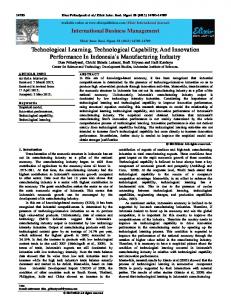
We tested in simulation how the model refinement approach, the discretization routine and the active learning algorithm perform together. We performed experiments at the PickUp task. The robot was skilled at picking up objects of spherical and cuboidal shapes. It could lift objects of the smaller size and those that weighed less than half a pound. Fig. 5.7 represents the true Capability Model for this simulated robot.

Shape

Size

Weight

SIT = {Size, Shape, Weight, Arm} CNTX = {Size, Shape, Weight}, COMM = {Arm} OUT = {Pick }, ATT = {} (b)

Arm

Pick

(a)

Arm  {Left, Right}, Shape ∈ {Sphere, Cuboid, Cylinder, Pyramid }, Size ∈ {Small, Large}, Weight ∈ {Light:[0,0.5], Heavy:[0.5,1]}, Pick ∈ {Success, Failure}, (c)

Figure 5.7: Capability Model of the simulated robot for the PickUp task. (a) depicts the Bayesian Network, (b) shows the type of each variable in the model and, (c) describes the values each variable can take.

We performed multiple runs of our algorithm with two different initial model guesses. Fig. 5.9a and 5.9b illustrate the results. Curves in blue show the learning trends when initialized with the model shown in Fig. 5.8. The curves in green depict the learning trends when the initial guess of the model includes the right set of variables with the appropriate discretization. Almost 80% of the time the algorithm correctly identifies all the relevant variables to include, the redundant variables to discard and the appropriate discretization for the variables in the model. However, 20% of the times, the algorithm either misses to discard a redundant variable, or is unable to identify a missing relevant variable, or fails to find the right discretization. 37

CHAPTER 5. EXPERIMENTS

Shape

Object Size Color

SIT = {ObjectPose, SurfaceFinish, Weight, Arm} CNTX = {ObjectPose, SurfaceFinish, Weight}, COMM = {Arm} OUT = {Pick }, ATT = {Size, Shape, ObjectColor } (b)

Arm

Pick

Object

Surface

Pose

Finish

(a)

Weight

Arm ∈ {Left,Right}, Shape ∈ {Sphere, Cuboid, Cylinder, Pyramid }, Size ∈ {Small, Large}, ObjectPose ∈ {Horizontal, Vertical }, ObjectColor ∈ {Red, Green, Blue}, SurfaceFinish ∈ {Smooth, Rough}, Weight ∈ {W:[0,1]}, Pick ∈ {Success, Failure}, (c)

Figure 5.8: Initial guess of the Capability Model for the PickUp task. (a) depicts the Bayesian Network, (b) shows the type of each variable in the model and, (c) describes the values each variable can take.

(a) Learning trends for runs that converged to the correct model

(b) Learning trends for runs that converged to an incorrect model

Figure 5.9: (a) and (b) depict the trend in DKL (Pθpredefined (KDo)||PθPickUp (KDo)). The curves in blue depict the trends for the learner’s model as it identifies the relevant factors, red points mark instances when a new variable is added, yellow points mark instances when a variable is removed from the model and purple points mark instances when a cutpoint is chosen for a continuous variable. The curves in green depict the trend if the model were initialized with the right variables. 38

CHAPTER 5. EXPERIMENTS

5.4

Quantifying Capabilities

We programmed a Pepper robot (Fig. 4.6b) to detect and pickup objects of three shapes viz. spherical, cuboidal and cylindrical. We experimented with two sets of weights and two sizes for each shape (in total 12 types of objects). Fig. 5.10 depicts the Capability Model of Pepper at the PickUp task. A Context (Size, Shape and Weight) denotes an object type. In every experiment Pepper was asked to pick up a particular type of object with one of its arms.

Shape

Weight

Size

SIT = {Shape, Size, Weight, Arm} CNTX = {Shape, Size, Weight}, COMM = {Arm} OUT = {Pick }, ATTPick = {} (b)

Arm

Pick

(a)

Arm ∈ {Left, Right}, Shape ∈ {Sphere, Cuboid, Cylinder }, Size ∈ {Small, Large}, Weight ∈ {Light, Heavy}, Pick ∈ {Success, Failure}, (c)

Figure 5.10: Capability Model for the Pickup task. (a) depicts the Bayesian Network, (b) shows the type of each variable in the model and, (c) describes the values each variable can take.

We performed 2 trials with 70 experiments each to learn the conditional probability tables associated with the Capability Model. We computed Score, as defined in Eq. PickUp (3.13), for each object type using the reference Pref defined in Eq. (5.1). We identified object types with score higher than a threshold at the end of both trials, as favourable for Pepper to pickup. ( PickUp Pref (Pick |Arm) =

1 if Pick = Success 0 otherwise

(5.1) 39

CHAPTER 5. EXPERIMENTS Having knowledge of the scenarios a robot is well suited for could help in a collaborative task. To demonstrate this, we employed the robot along with a human to clear a cluttered table. In every experiment, the human cleared all but 4 objects off the table and, the robot had to clear the rest. The robot was allowed 3 tries per object (12 in total). We performed such experiments in two settings. In the first setting, the human randomly selected objects for the robot to pick up and in the second, the human only selected objects of favourable types. We conducted 5 experiments in each setting. Table 5.1 summarizes the results. Settings

Number of objects cleared

Number of tries

Objects of any type

1.8 ± 0.98

8.8 ± 1.7

Objects of favourable types

3.4 ± 0.49

6.6 ± 1.2

Table 5.1: Results of the clear-the-table task (µ ± σ) after 5 experiments per setting. Performance at the task is better in terms of number of tries as well as number of objects cleared, when the robot is employed in a favourable scenario.

5.5

Summary

The contributions of this thesis can be summarized as follows • We presented Capability Model, a framework to capture a robot’s ability to

perform a task. This framework incorporates uncertainity inherent to physical systems (robots) as well as the effect of extrinsic factors on a robot’s capability. • We developed an algorithm to build Capability Models from active experi-

mentation. Our algorithm identifies relevant extrinsic factors from a list of possibilities. Moreover, it quantifies the robot’s ability to accomplish the task in different settings of these factors. • We introduced a metric to identify favourable scenarios for deploying a robot

to carry out a particular task. • We illustrated a method for drawing inferences from a robot’s appearance

about the different tasks it can potentially perform. Our algorithm for building Capability Model for a task requires a list of possibly relevant extrinsic factors. We proposed requesting a human to provide this list. We discussed results of a 40

CHAPTER 5. EXPERIMENTS survey we conducted to evaluate how accurately people identify extrinsic factors that affect a robot’s capability at a task. A video describing our work can be found here.

41

CHAPTER 5. EXPERIMENTS

42

Chapter 6 Conclusions and Future Work As robots become increasingly multifunctional, it becomes difficult to ascertain what tasks they can perform and how good they are at those tasks. To the best of our knowledge, inferring capabilities from appearance and active experimentation is a novel problem. We proposed a method to build models of a robot’s capabilities and presented experiments with a NAO and a Pepper robot performing two different tasks. We demonstrated the utility of such models in working collaboratively with a robot. Some interesting future directions are as follows, • Robots are capable of learning new skills and adapting to new scenarios over

time. However, there are certain limitations a robot can never learn to overcome. For example, a robot can learn new ways to grasp enabling it to pick up a wider range of objects but, it can never lift anything that weighs beyond its physical limitations. How do we incorporate this knowledge into our learning routine or learn to identify factors that are intrinsically limiting? • A robot’s spec sheet presents information about the sensors and actuators used

to build the robot. This information can be useful in determining the tasks a robot can perform and its physical limitations (Field of view, sensing range, actuation limits, etc.). How do we utilize this information in building models? • We assumed that experimenting with a robot in any Situation has the same

cost. Depending on the task, this may be quite far from reality. How do we learn models in such scenarios?

43

CHAPTER 6. CONCLUSIONS AND FUTURE WORK

44

Chapter 7 Appendix 7.1

CutValue Maximization

Consider a simple network as shown in Fig. 7.1. Without loss of generality as?X sume Domain(X) = (0,1). Furthermore, U?X = (u?X 1 , · · · , um ) and, P (O|X) = Pi if DU?X (X) = i such that Pi 6= Pi+1 . We show that cutpoints in U?X are local maximas of CutValue (Section 3.2.3, Eq. (3.9)). Therefore, the sequnce UX built by greedily picking cutpoints based on their CutValue is infact U?X .

X

O

Figure 7.1: Example Bayesian Network. X is continuous and O is discrete.

?X Assume UX = (). Consider a cutpoint u ∈ (u?X j , uj+1 ) and the subsequent sequence UX obtained after adding u to UX .

45

CHAPTER 7. APPENDIX

CutValue(UX , UX ) = I(O; X|UX ) − I(O; X|UX ) (7.1) Z Z = H(P (O|X, UX ))P (X|UX ) − H(P (O|X, UX ))P (X|UX ) X ZX X X = H(P (O|X, U ))P (X|U ) − F (u) (7.2) X

F (u) =

R X

H(P (O|X, UX ))P (X|UX ) is the only term that depends on UX = (u),

F (u) = H(P (O|X ≤ u))P (X ≤ u) + H(P (O|X > u))P (X > u) = H(P (O|X ≤ u))u + H(P (O|X > u))(1 − u)

(7.3)

From our assumption about the distribution of O, we can simplify H(P (O|X ≤ u)) and H(P (O|X > u)) as follows

P (O|X ≤ u) =

j−1 X i=0

?X (u − u?X (u?X j ) i+1 − ui ) Pi + Pj (where u?X 0 = 0) u u

m X (u?X (u?X − u?X j+1 − u) i ) + Pi i+1 (where u?X P (O|X > u) = Pj m+1 = 1) 1−u 1 − u i=j+1

(7.4)

(7.5)

Therefore,

 Pj−1 (u?X − u?X )Pi + (u − u?X )Pj  i+1 i j i=0 F (u) =uH + u P  (u?X − u)Pj + m (u?X − u?X )Pi  j+1 i i=j+1 i+1 (1 − u)H 1−u

(7.6)

?X ?X In the interval (u?X j , uj+1 ), F (u) is concave with the lowest value at either uj or u?X j+1 . We can show this by considering the following

46

CHAPTER 7. APPENDIX

h  Pj−1 (u?X − u?X )Pi (o) + (u − u?X )Pj (o)  i+1 i j i=0 Pj (o) log (7.7) u o∈Domain(O)  i 1−u Pm + log ?X ?X (u?X j+1 − u)Pj (o) + i=j+1 (ui+1 − ui )Pi (o)

dF (u) =− du

X

dF (u) du

?X keeps decreasing as u goes from u?X j to uj+1 . Thus F (u) is minimum (and X ?X the CutValue(UX , UX ) maximum) at u = u?X j or u = uj+1 . Here, we considered U to be empty however, the approach is exactly the same for a non-empty UX .

Fig. 7.2 shows the CutValue for different possible cutpoints for two different U . In this example, U?X = (0.3, 0.6, 0.9). As can be seen, u = 0.3 has the highest CutValue when UX is empty. When u = 0.3 is incorporated, we still see local maximas at the true cutpoints. This example demonstrates that greedily picking cutpoints yields the true sequnce. X

Figure 7.2: Trend in CutValue(UX , UX ) for two different UX . The dotted lines ?X indicate u?X = (0.3, 0.6, 0.9) i , U

When the set OUT is not singleton, the analysis is similar 47

CHAPTER 7. APPENDIX

CutValue(UX , UX ) =

X

I(O; X|UX ) − I(O; X|UX )

O∈OUT

=

X Z O∈OUT

H(P (O|X, UX ))P (X|UX )−

X

Z

 H(P (O|X, UX ))P (X|UX )

(7.8)

X

As O ∈ OUT are independent given X, P (OUT|X) = ΠO∈OUT P (O|X). Therefore, P H(P (OUT|X, UX )) = O∈OUT H(P (O|X, UX )).

X

Z

X

X

X

Z

H(P (OUT|X, U ))P (X|U ) −

CutValue(U , U ) = ZX =

H(P (OUT|X, UX ))P (X|UX )

X

H(P (OUT|X, UX ))P (OUT|UX ) − F (u)

(7.9)

X

When the set OUT has additional dependencies, the analysis is not that simple.

48

Chapter 8 Bibliography [1] Adrien Baran`es and Pierre-Yves Oudeyer. R-iac: Robust intrinsically motivated exploration and active learning. IEEE Transactions on Autonomous Mental Development, 1(3):155–169, 2009. 2 [2] Adrien Baranes and Pierre-Yves Oudeyer. Active learning of inverse models with intrinsically motivated goal exploration in robots. Robotics and Autonomous Systems, 61(1):49–73, 2013. 2 [3] Anthony Dearden, Yiannis Demiris, LP Kaelbling, and A Saffotti. Learning forward models for robots. IJCAI-INT JOINT CONF ARTIF INTELL. 2 [4] Usama Fayyad and Keki Irani. Multi-interval discretization of continuous-valued attributes for classification learning. 1993. 3.2.3 [5] S. Forestier and P. Y. Oudeyer. Modular active curiosity-driven discovery of tool use. In 2016 IEEE/RSJ International Conference on Intelligent Robots and Systems (IROS), pages 3965–3972, Oct 2016. doi: 10.1109/IROS.2016.7759584. 2 [6] S´ebastien Forestier, Yoan Mollard, and Pierre-Yves Oudeyer. Intrinsically motivated goal exploration processes with automatic curriculum learning. CoRR, abs/1708.02190, 2017. URL http://arxiv.org/abs/1708.02190. 2 [7] Nir Friedman, Moises Goldszmidt, et al. Discretizing continuous attributes while learning bayesian networks. 3.2.3 [8] Yolanda Gil. Learning by experimentation: Incremental refinement of incomplete planning domains. In Proceedings of the Eleventh International Conference on International Conference on Machine Learning, ICML’94, pages 87–95, San Francisco, CA, USA, 1994. Morgan Kaufmann Publishers Inc. ISBN 1-55860335-2. URL http://dl.acm.org/citation.cfm?id=3091574.3091586. 2 [9] K. He, X. Zhang, S. Ren, and J. Sun. Deep residual learning for image recognition. 49

Bibliography In 2016 IEEE Conference on Computer Vision and Pattern Recognition (CVPR), pages 770–778, June 2016. doi: 10.1109/CVPR.2016.90. 4.1 [10] S. Hfer and O. Brock. Coupled learning of action parameters and forward models for manipulation. In 2016 IEEE/RSJ International Conference on Intelligent Robots and Systems (IROS), pages 3893–3899, Oct 2016. doi: 10.1109/IROS. 2016.7759573. 2 [11] James J. Gibson. The theory of affordances chapt. 8., 01 1977. 2 [12] Michael I Jordan and David E Rumelhart. Forward models: Supervised learning with a distal teacher. Cognitive science, 16(3):307–354, 1992. 2 [13] Minae Kwon, Malte F Jung, and Ross A Knepper. Human expectations of social robots. In The Eleventh ACM/IEEE International Conference on Human Robot Interaction, pages 463–464. IEEE Press, 2016. 4.1 [14] Tom M Mitchell, Paul E Utgoff, and Ranan Banerji. Learning by experimentation: Acquiring and refining problem-solving heuristics. In Machine Learning, Volume I, pages 163–190. Elsevier, 1983. 2 [15] Bogdan Moldovan, Plinio Moreno, Martijn van Otterlo, Jos´e Santos-Victor, and Luc De Raedt. Learning relational affordance models for robots in multiobject manipulation tasks. In Robotics and Automation (ICRA), 2012 IEEE International Conference on, pages 4373–4378. IEEE, 2012. 2 [16] L. Montesano, M. Lopes, A. Bernardino, and J. Santos-Victor. Learning object affordances: From sensory–motor coordination to imitation. IEEE Transactions on Robotics, 24(1):15–26, Feb 2008. ISSN 1552-3098. doi: 10.1109/TRO.2007. 914848. 2 [17] J. Mugan and B. Kuipers. Autonomous learning of high-level states and actions in continuous environments. IEEE Transactions on Autonomous Mental Development, 4(1):70–86, March 2012. ISSN 1943-0604. doi: 10.1109/TAMD.2011. 2160943. 2 ¨ coluk. [18] Erol S¸ahin, Maya C ¸ akmak, Mehmet R Do˘gar, Emre U˘gur, and G¨okt¨ urk U¸ To afford or not to afford: A new formalization of affordances toward affordancebased robot control. Adaptive Behavior, 15(4):447–472, 2007. 2 [19] Paul D. Scott and Shaul Markovitch. Experience selection and problem choice in an exploratory learning system. Machine Learning, 12(1):49–67, Aug 1993. ISSN 1573-0565. doi: 10.1007/BF00993060. URL https://doi.org/10.1007/ BF00993060. 2 [20] Simon Tong and Daphne Koller. Active learning for parameter estimation in bayesian networks. In Proceedings of the 13th International Conference on Neural Information Processing Systems, NIPS’00, pages 626–632, Cambridge,

50

Bibliography MA, USA, 2000. MIT Press. URL http://dl.acm.org/citation.cfm?id= 3008751.3008842. 3.2.1, 3.2.1 [21] C. Wang, K. V. Hindriks, and R. Babuska. Active learning of affordances for robot use of household objects. In 2014 IEEE-RAS International Conference on Humanoid Robots, pages 566–572, Nov 2014. doi: 10.1109/HUMANOIDS.2014. 7041419. 2

51