is a step up from Burger King, and she will probably appreciate the more congenial atmosphere. In the predator{prey domain, such a situation is shown in Figure ...
Learning Cases to Compliment Rules for Con ict Resolution in Multiagent Systems Thomas Haynes, Kit Lau & Sandip Sen Department of Mathematical & Computer Sciences, The University of Tulsa e-mail: [haynes,laukit,sandip]@euler.mcs.utulsa.edu
Abstract Groups of agents following xed behavioral rules can be limited in performance and e�ciency. Adaptability and exibility are key components of intelligent behavior which allow agent groups to improve performance in a given domain using prior problem solving experience. We motivate the usefulness of individual learning by group members in the context of overall group behavior. We propose a framework in which individual group members learn cases to improve their model of other group members. We utilize a testbed problem from the distributed AI literature to show that simultaneous learning by group members can lead to signi cant improvement in group performance and ef ciency over groups following static behavioral rules.
Introduction
We are actively engaged in research on multiagent interactions (Haynes et al. 1995a; 1995b; Sen, Sekaran, & Hale 1994), and in particular, con ict resolution between agents for critical resources. This research has shown that agents need to interact on{line in order to learn e�ective cooperation; xed behavioral rules do not usually encompass all possible interactions. By examining why a con ict occurred, an agent is able to modify its behavioral rules such that that con ict does not occur again in the future. We utilize the predator{prey domain (Haynes et al. 1995a; Korf 1992; Stephens & Merx 1990) to demonstrate a typical con ict resolution scenario. The goal of the four predator agents is to try to capture a prey agent. Agents can only make orthogonal moves on a grid world. We have reported the varying degrees of success of predator agents in capturing a prey against a variety of prey movement algorithms (Haynes et al. 1995a). Of particular interest were the algorithms which caused the prey to pick a direction and always move along it (Linear) and the one in which it did not move at all (Still). All the predator strategies we investigated failed against at least one of these prey strategies. In this paper we investigate how case{based
learning will allow the predators to capture preys employing these algorithms. The behavioral strategies of the predators use one of two distance metrics: Manhattan distance (MD) and max norm (MN). The MD metric is the sum of the differences of the x and y coordinates between two agents. The MN metric is the maximum of the di�erences of the x and y coordinates between two agents. The algorithms examine the metrics from the set of possible moves, fN,E,S,W,Hg, and select a move corresponding to the minimal distance. All ties are randomly broken. The original MN algorithm, as described by Korf (Korf 1992), does not allow the predators to move to the cell occupied by the prey. (In his research, the prey moves rst, followed by the predators in order. Thus con icts are resolved between predators and prey by serialization.) Figure 1 illustrates a problem with this restriction. The cells to the North and South of predator 4 are as equally distant from the prey P as the cell currently occupied by predator 4. Since all ties are non{deterministically broken, with each movement of the agents, there is a 66% probability that predator 4 will allow the prey P to escape. Assuming a Linear prey moving East, Figure 1 also illustrates the failure of the MN metric algorithms to capture a Linear prey. It is possible that a predator can manage to block the prey, but it is not very likely that it can keep the prey blocked long enough for a capture to take place. It is also possible that once captured, the prey may escape the MN metric algorithms. The MD metric algorithms do not su�er from this inability to make stable captures. They do however have a drawback which both the Linear and Still prey algorithms expose. We found that MD metric algorithms stop a Linear prey from advancing. Our original hypothesis was that the Linear prey moved in such a manner so as to always keep the predators \behind" it. Thus, the inability to capture it was due to not stopping its forward motion. We started keeping track of blocks, i.e., a 1 situation in which a predator blocks the motion of the
prey, and discovered that the MD metric algorithms were very good at blocking the Linear prey. Why then can they not capture it? The answer lies in the fact that the MD metric algorithms are very susceptible to deadlock situations. If, as in Figure 2(a), a predator manages to block a Linear prey, it is typical for the other predators to be strung out behind the prey. The basic nature of the algorithm ensures that positions orthogonal to the prey are closer than positions o� the axis. Thus, as shown in Figures 2(b) and (c), the remaining predators manage to close in on the prey, with the exception being any agents who are blocked from further advancement by other agents. The greedy nature of these algorithms ensures that in situations similar to Figure 2(c), neither will predator 2 yield to predator 3 nor will predator 3 go around predator 2. While the MN metric algorithms can perform either of these two actions, they are not able to keep the Linear prey from advancing. It is also evident that once the Linear prey has been blocked by a MD metric algorithm, the prey algorithm degenerates into the Still algorithm. This explains the surprising lack of captures for a prey which does not move. The question that arises from these ndings is how do the agents manage con ict resolution? An answer can be found in the ways we as humans manage con ict resolution: with cases (Kolodner 1993). In the simplest sense, if predator 1 senses that if predator 2 is in its Northeast cell, and it has determined to move North, then if the other agent moves West there will be a con ict with predator 2. predator 1 should then learn that in the above situation, it should not move North, but rather to its next most preferable direction. In this research we examine case based learning (CBL) of potential con icts, which will allow agents to avoid those con icts. The default rule employed by predators is to move closer to the prey, unless an overriding case is present. If a case res, the next best move is considered. If the suggested move, either by the default rule or a case ring, does not succeed, then a new case is learned.
Motivation for Learning Cases
For the majority of moves in the predator{prey domain, either the max norm or MD metric algorithms su�ce in at least keeping the predator agents the same distance away from the prey. As discussed later, the prey e�ectively moves 10% slower than the predators, the grid world is toroidal and the prey must occasionally move towards some predators to move away from others. Therefore the predators will eventually catch up with it. Contention for desirable cells begins when the predators either get close to the prey or are bunched
1 2 B
(a)
3 4 1 2 B
(b)
Figure 3: Con icts in ring lanes for ghter planes stra ng a bomber. (a) ghter 1 is blocked from ring by ghter 2, and (b) Not only is ghter 1 blocked, but so is ghter 3 by ghter 4. up on one of the orthogonal axes. What the predators need to learn is table manners. Under certain conditions, i.e. when two or more predator agents vie for a cell, the greedy nature of the above algorithms must be overridden. We could simply order the movements of the predators, allowing predator 1 to always go rst. But it might not always be the fastest way to capture the prey. No ordering is likely to be more economical than others under all circumstances. Also, if we consider real world predator{prey situations, the arti cial ordering cannot always be adhered to. Consider for example a combat engagement between ghter aircraft and a bomber. If there are only two ghters, the ordering rule suggests that ghter 1 always moves before ghter 2. If they are in the situation depicted in Figure 3(a), then ghter 1 cannot re on the bomber B, because doing so will hit ghter 2. Clearly, ghter 2 should rst move North or South, allowing both it and the other ghter to have clear re lanes. But under the proposed ordering of the movements, it cannot move in such a manner. So, the default rules is that ghter 1 moves before ghter 2, with an exception if ghter 2 is in front of ghter 1. The rule can be modi ed such that the agent in front gets to move rst. However, if we add more ghters, then the situation in Figure 3(b) does not get handled very well. How do ghter 2 and ghter 4 decide who shall go rst? What if they both move to the same cell North of ghter 2? These are the very problems we have been discussing with the MD metric algorithm. What is needed is a dynamic learning mechanism to model the actions of other agents. Until the potential for con icts exist, agents need not be concerned with the speci c model of other agents. It is only when a con ict occurs that an agent learns that another agent will \act" a certain way in a speci c situation Si . Thus rst agent learns not to employ its default rule in situation Si ; instead it considers its next best action. As 2
1 3 2
P 4
(a)
1 3 P 4 2
1 4 3 P 2
(b)
(c)
Figure 1: A possible sequence of movements in which a MN metric based predator tries to block the prey P. (a) predator 4 manages to block P. Note that 4 is just as likely to stay still as move North or South. (b) predators 1 and 3 have moved into a capture position, and predator 2 is about to do so. Note that 4 is just as likely to stay still as move North or South. (c) predator 4 opts to move to the North, allowing the prey P to escape. Note that 4 is just as likely to stay still as move East or West. 1 3 2
P 4
1 3 2 P 4
1 3 2 P 4
(b)
(c)
(a)
Figure 2: A possible scenario in which a MD metric based predator tries to block the prey P. (a) predator 4 manages to block P. predators 1, 2, and 3 move in for the capture. (b) predator 2 has moved into a capture position. (c) predator 1 has moved into a capture position. predator 2 will not yield to predator 3. They are in deadlock, and the prey P will never be captured. these speci c situations are encountered by an agent, it forms a case base library of con icts to avoid. The agents learning the cases, or situations, is beginning to model the actions of others. The growing case{base library allows an agent to better coordinate its actions with that of other agents in the group.
Enhanced Behavioral Rules
In order to facilitate e�cient capture, i.e., provide the agents with the best set of default rules, we enhanced the basic MD algorithm. This will also provide a better challenge for the learning algorithm to improve on. If we consider human agents playing a predator{prey game, we would see more sophisticated reasoning than simple greedy behavioral rules. When faced with two or more equally attractive actions, a human will spend extra computational e�ort to break the tie. Let us introduce some human agents: Alex, Bob, Cathy, and Debbie. Bob and Debbie have had a ght, and Bob wants to make up with her. He asks Alex what should he do. Alex replies that in similar situations he takes Cathy out to dinner. Bob decides that either Burger
King or Denny's will do the trick (He is a college student, and hence broke most of the time). In trying to decide which of his two choices is better, he predicts how Debbie will react to both restaurants. Denny's is a step up from Burger King, and she will probably appreciate the more congenial atmosphere. In the predator{prey domain, such a situation is shown in Figure 4(a). Predator 1 has a dilemma: both of the cells denoted by x and y are 2 cells away from Prey P, using the MD metric. The sum of the distances between all the possible moves from x and Prey P is 8 and the sum from y to the Prey P is 10. Therefore using this algorithm, which we call the look ahead tie{breaker, predator 1 should chose x over y. A second re nement comes from what happens if the look ahead tie{breaker yields equal distances for x and y? Such a scenario is shown in Figure 4(b). Then predator 1 should determine which of the two cells is less likely to be in contention with another agent. Predators do not mind contending for cells with the prey, but they do not want to waste a move bouncing o� of another predator. By the least con ict tie{breaking 3
P x 1 y
2 x P 1 y
(a)
(b)
Figure 4: In both (a) and (b), the cells marked x and y are equal distant via the MD metric from the Prey P for predator 1. (a) x is chosen because the sum of the possible moves from it to Prey P is less than the y's sum of moves, and in (b) y is chosen because while the look ahead is equal, there is a potential for con ict with predator 2 at x. algorithm, predator 1 should pick y over x (y has 0 contentions, while x has 1). Suppose that Bob and Debbie have had another ght, but this time Alex and Cathy also have fought. Furthermore, a new restaurant, the Kettle, has opened up in town. Since the Kettle is on par with Denny's, Bob is again faced with a need to break a tie. As he knows that Alex and Cathy have fought, he believes that Alex will be taking her out to make up with her. Bob does not want to end up at the same restaurant, as he and Debbie will have to join the other couple, which is hardly conducive to a romantic atmosphere. He decides to model Alex's behavior. Like Bob, Alex is a student and has never eaten at the Kettle. Since Cathy is placated by being taken to Denny's and Alex does not like changing his routine, then Alex will most likely take her there. Thus Bob decides to take Debbie to the Kettle. Notice that if Bob had not accounted for a change in the environment, then his case would have caused a con ict with his goal.
Case Representation and Indexing
The ideal case representation for the predator{prey domain is to store the entire board and to have each case inform all predators where to move. There are two problems with this setup: the number of cases is too large, and the agents do not act independently. Each agent could store this case library independently, but the problem size explodes. An e�ective \case window" for each predator is to represent all cells that could directly cause con icts with any move taken by the agent, as shown in Figure 5. A drawback to this approach is that agents can be present in the case window, but not actually be part of the case. For example, predator 2's location does not impact the desired move of East for predator 4 in Figure 5. Another problem with
P 2
4
1 3
Figure 5: Representation of a simple case window for
predator 4.
X P 2 1 (a)
X P 1 2 (b)
Figure 6: Representation of cases for predator 1 in the example: (a) Moving (note predator 2 is outside the case window), and (b) Staying still. The X denotes which of the three areas the prey is occupying. this window is that predator 2 could be just North of predator 1, and cause either predator 1 or prey P to move di�erently than in the scenario presented. Finally, the search space is still too large. Unless the full board is used as a case, any narrowing of the case window is going to su�er from the rst two points of the e�ective case window presented above. This is symptomatic of an \open" and \noisy" domain: the same case can represent several actual con gurations of the domain being modeled. The price to pay to have a clean case base is in the size of the search space. If we accept that the case windows are going to map to more than one physical situation, then clearly the issue is how to make the search space manageable. The case window in Figure 5 encompasses the potential con icts when the agent moves in any of the allowable directions. If we limit the case window to simply represent the potential con icts that can occur \after" the agent selects a move based on the default rules or learned case, then we can utilize the case windows shown in Figure 6. The case window in Figure 6(a) is rotationally symmetric for the directions the agent can choose, and the case window in Figure 6(b) is applied for when the agent remains stationary. Our cases are negative in the sense they tell the agents what not to do. A positive case would tell the agent what to do in a certain situation (Golding & Rosenbloom 1991). Each case contains information 4 describing the contents of the four cells which have ac-
1 Preferentially order actions by behavioral rules. 2 Choose the rst action which does not cause a
negative case to re, i.e., one containing a con ict. 3 If the state corresponding to the selected action is not reached, then the agent must learn a case.
Figure 7: Algorithm for selecting actions based on negative cases. cess to the cell which the agent wants to occupy in the next time step. The other crucial piece of knowledge needed is where does the agent believe the other agents are going to move? This is modeled by storing the orientation of the prey's position with respect to the desired direction of movement of the agent. Speci cally, we store whether the prey lies on the agent's line of advance or if it is to the left or right of the line. An agent has to combine its behavioral rules and learned cases to choose its actions. The algorithm for doing so is shown in Figure 7. In the predator{prey domain, to index a case, the agent determines whether the possible action is for movement or staying still. As discussed above, this decision determines the case library to accessed. Then it examines the contents of each of the four cells which can cause con icts. The contents can be summed to form an unique integer index in a base number system re ecting the range of contents. The rst possible action which does not have a negative case is chosen as the move for that turn. We used case windows as shown in Figure 6 while learning to capture the Still prey. The results were promising, but we found that the predators would falsely learn cases, which hindered the e�cient capture of the prey. Such an erroneous scenario is shown in Figure 8. The problem lies in predator 1's interpretation of the scenario. It tried to move to the location of prey P and failed. It does not learn in situations involving prey P. Now predator 2 pushes predator 1, and predator 1 should learn to yield to predator 2 if it is again faced with the situation shown in Figure 8(a). The case it learns is the stationary case window shown in Figure 6(b). This case informs predator 1 that if its current best action is to stay still, then it should consider the next best action. However, this case will never re because predator 1's best action is to move into prey P's cell, and since the predators do not learn cases against the prey, there is no case that will cause it to consider its remaining actions. Thus the exact same con ict will occur, and predator 1 will re-learn the same case without ever applying it. The case that should be learned is that when predator 1 is in the situation depicted in Figure 8(a), then 5
P 1 2
P 1 2
(a)
(b)
1 P 2 (c)
Figure 8: predator 1 learns the wrong case. (a) predator 1's best action is to move towards prey P. (b) predator 1 bounces back from the prey P. It has now stored the incorrect fact that it has stayed still and not moved East. (c) predator 2 pushes out predator 1, and predator 1 learns the incorrect case that if its
best action is to stay still in the con guration shown in (a), then it should select its next best action. X P 2 1
Figure 9: New case window. Note it also shows predator 1's learned case from the example. it should consider its next best action. However, as can be seen in Figure 6(a), such a situation can not be learned with the current case windows. In order to capture the necessary information, we decided to merge the two case windows of Figure 6 into one, which is shown in Figure 9. Now agents can store cases in which there is a potential for con ict for both the resource it desires and the resource it currently possess. The learned case is shown in Figure 9. If the same situation, as in Figure 8(a), is encountered, the case will re and predator 1 will consider its next best action. With the enhanced rules, this will be to move North.
Experimental Setup and Results
The initial con guration consists of the prey in the center of a 30 by 30 grid and the predators placed in random non{overlapping positions. All agents choose their actions simultaneously. The environment is accordingly updated and the agents choose their next action based on the updated environment state. If two agents try to move into the same location simultaneously, they are \bumped back" to their prior positions. One predator, however, can push another predator (but not the prey) if the latter decided not to move. The prey does not move 10% of the time; e�ectively making the predators travel faster than the prey. The grid is toroidal
in nature, and only orthogonal moves are allowed. All agents can sense the positions of all other agents. Furthermore, the predators do not possess any explicit communication skills; two predators cannot communicate to resolve con icts or negotiate a capture strategy. The case window employed is that depicted in Figure 9. Initially we were interested in the ability of predator behavioral rules to e�ectively capture the Still prey. We tested three behavioral strategies: MD { the basic MD algorithm, MD{EDR { the MD modi ed with the enhancements discussed earlier, and MD{CBL { which is MD{EDR utilizing a case base learned from training on 100 random simulations. The results of applying these strategies on 100 test cases are shown in Table 1. While the enhancement of the behavioral rules does increase capture, the addition of negative cases leads to capture in almost every simulation. Algorithm MD MD{EDR MD{CBL
Captures 3 46 97
Ave. Number of Steps 19.00 21.02 23.23
Table 1: Number of captures (out of a 100 test cases) and average number of steps to capture for the Still prey. We also conducted a set of experiments in which the prey used the Linear algorithm as its behavioral rule. Again we tested the three predator behavioral strategies of MD, MD{EDR, and MD{CBL. The MD{ CBL algorithm was trained on the Still prey. We trained on a Still prey because the Linear prey typically degrades to a Still prey. We have also presented the results of training the MD{CBL on the Linear prey (MD{CBL? ). The results for the Linear prey are presented in Table 2. Algorithm MD MD{EDR MD{CBL MD{CBL?
Captures 2 20 54 36
Ave. Number of Steps 26.00 24.10 27.89 31.31
Table 2: Number of captures (out of a 100 test cases) and average number of steps to capture for the Linear prey. MD{CBL? denotes a test of the MD{CBL when trained on a Linear prey. With both prey algorithms, the order of increasing e�ectiveness was MD, MD{EDR, and MD{CBL. Clearly the addition of CBL to this multiagent system 6
is instrumental in increasing the e�ectiveness of the behavioral rules. There is some room for improvement, as the results from the Linear prey indicate. We believe that the decrease in capture rate for the MD{CBL? run was a result of the agents not being exposed to a su�cient number of distinct con ict situations. A majority of the time spent in capturing the Linear prey is spent chasing it. Only after it is blocked do interesting con ict situations occur.
Conclusions
We have introduced an algorithm which enables agents to learn how to enhance group performance. Default behavioral rules used to model the group interactions are extended by cases to account for con icting interests within the group. We also showed the utility of such a learning system in the predator{prey domain. We are hoping to further extend the system to allow the agents to forget cases which no longer apply due to the dynamical nature of the acquisition of knowledge.
References
Golding, A. R., and Rosenbloom, P. S. 1991. Improving rule{based systems through case{based reasoning. In Proceedings of the Ninth National Conference on Arti cial Intelligence, 22{27. Haynes, T.; Sen, S.; Schoenefeld, D.; and Wainwright, R. 1995a. Evolving multiagent coordination strategies with genetic programming. Arti cial Intelligence. (submitted for review). Haynes, T.; Wainwright, R.; Sen, S.; and Schoenefeld, D. 1995b. Strongly typed genetic programming in evolving cooperation strategies. In Eshelman, L., ed., Proceedings of the Sixth International Conference on Genetic Algorithms, 271{278. San Francisco, CA: Morgan Kaufmann Publishers, Inc. Kolodner, J. L. 1993. Case{Based Reasoning. Morgan Kaufmann Publishers. Korf, R. E. 1992. A simple solution to pursuit games. In Working Papers of the 11th International Workshop on Distributed Arti cial Intelligence, 183{194. Sen, S.; Sekaran, M.; and Hale, J. 1994. Learning to coordinate without sharing information. In Proceedings of the Twelth National Conference on Arti cial Intelligence, 426{431.
Stephens, L. M., and Merx, M. B. 1990. The e�ect of agent control strategy on the performance of a DAI pursuit problem. In Proceedings of the 1990 Distributed AI Workshop.