Learning cluster-based structure to solve constraint ... - CiteSeerX

Ann Math Artif Intell DOI 10.1007/s10472-010-9212-z

Learning cluster-based structure to solve constraint satisfaction problems Xingjian Li · Susan L. Epstein

© Springer Science+Business Media B.V. 2010

Abstract The hybrid search algorithm for constraint satisfaction problems described here first uses local search to detect crucial substructures and then applies that knowledge to solve the problem. This paper shows the difficulties encountered by traditional and state-of-the-art learning heuristics when these substructures are overlooked. It introduces a new algorithm, Foretell, to detect dense and tight substructures called clusters with local search. It also develops two ways to use clusters during global search: one supports variable-ordering heuristics and the other makes inferences adapted to them. Together they improve performance on both benchmark and real-world problems. Keywords Cluster · Structure learning · Hybrid search · Constraint satisfaction problem Mathematics Subject Classification (2010) 68T20 1 Introduction A problem solver that begins with a general algorithm for search may well be surprised, or even defeated, by difficult subproblems that lurk within the larger one.

X. Li (B) · S. L. Epstein Department of Computer Science, The Graduate Center of The City University of New York, New York, NY 10016, USA e-mail: [email protected] S. L. Epstein Department of Computer Science, Hunter College of The City University of New York, New York, NY 10065, USA e-mail: [email protected]

X. Li, S.L. Epstein

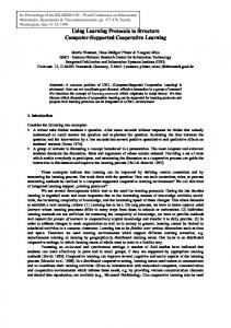
Indeed, many modern algorithms are now designed to learn about such subproblems during search, as they encounter them. The thesis of this paper, however, is that it is possible, and better, to identify such subproblems before search, and then exploit them both to solve and to understand the problem at hand. The principle result of this paper is that it is feasible to detect difficult subproblems within a challenging constraint satisfaction problem (CSP) and then exploit a structure composed of them, both to solve the CSP effectively and to explain it to a user. On certain benchmark problems, this approach achieves as much as an order of magnitude speedup. Moreover, the learned structure provides a meaningful high-level formulation of the problem. Search-ordering heuristics can be misled if they overlook the inherent structure of a problem. A binary CSP, for example, has a set of variables, each with a domain of values, and a set of constraints, each of which restricts how some pair of variables can be bound simultaneously. Such a problem is often represented as a graph where each variable is a node and each constraint is an edge between the pair of variables it restricts. When search for a CSP’s solution assigns values to variables one at a time, the order in which the variables are addressed is crucial to search performance. Such search is typically supported by variable-ordering heuristics that prefer variables of high degree in the associated graph. Difficult subproblems, however, are not necessarily characterized by such variables. What is really needed is an effective reasoning mechanism that predicts and exploits difficult subproblems. The traditional graph in Fig. 1a, for example, plots its 200 variables on a circle, and offers little insight or guidance to a solver. Figure 1b redraws Fig. 1a by extracting some variables from the central circle, and Fig. 1c darkens the more restrictive constraints. This formulation is clear only to the problem generator, however. Without the knowledge in Fig. 1c, the problem could not be solved in 30 min by a traditional heuristic. Two learning heuristics (described below) solved it in about 127 and 88 s. This paper develops algorithms that detected the graph in Fig. 1d and used it to solve the same problem, all in 3.56 s. Although many challenging real-world problems can be modeled as CSPs, their graphs often have non-random structure that makes them difficult to solve for heuristics that ignore it. Here, a cluster in a CSP is a subproblem that is particularly difficult

Fig. 1 A cluster graph predicts subproblems crucial to search. a An uninformative graph for a CSP places the variables on the circumference of a circle. b The hidden structure of the same problem, given perfect knowledge. c Darker edges represent tighter constraints in the same problem. d A cluster graph displays critical portions of the problem. This graph was detected from (a) by local search

Cluster-based structure to solve constraint satisfaction problems

to solve, and a cluster graph is a structural model that illustrates the relationships among all a CSP’s discovered clusters. The next section provides background and formal definitions for constraint satisfaction problems and search for solutions to them. Section 3 describes related work on structure, while Section 4 investigates how perfect structural foreknowledge like Fig. 1c might best be used during search. Section 5 describes Foretell, a local search algorithm that detects clusters; Section 6 provides cluster graphs for several interesting CSPs. Section 7 explores several variable-ordering heuristics that are based on structural knowledge learned by Foretell. Section 8 investigates how such structural knowledge can be used in constraint inference; Section 9 provides experimental results for these algorithms on benchmark and read-world problems. The final section discusses the results and future work.

2 Background Constraint satisfaction searches for a solution to a problem that satisfies a set of restrictions. Many combinatoric problems, such as scheduling, can be represented as CSPs. Because CSP solution is NP-complete [26], no general-purpose polynomial time algorithm is likely to exist. Instead, much work has been directed toward the design of algorithms with shorter average run-times. This section introduces basic CSP terminology and some relevant search methods. 2.1 Constraint satisfaction problems A constraint satisfaction problem is represented by a triple < X, D, C >, where: • • •

X is a set of variables, X = {X1 , . . . , Xn } The domain of variable Xi is a finite and discrete set of its possible values Di ∈ D C is a set of constraints that restrict the values the variables in it scope Si ⊆ X can hold simultaneously

A constraint Ci uses a relation Ri to indicate which tuples in the Cartesian product of the domains of the variables in Si are acceptable. If Ci is extensional, Ri enumerates the tuples; if Ci is intensional, Ri is a boolean predicate over all the tuples. This paper deals primarily with extensional CSPs, all of whose constraints are extensional. (Some empirical results on intensional CSPs, all of whose constraints are intensional, appear in Section 9.) A subproblem < V, D# , C# > of a CSP < X, D, C > is a CSP induced by a subset of variables V ⊆ X, where D# = {Di ∈ D|Xi ∈ V} and C# = {Ci |Si is the scope of Ci and Si ⊆ V}. The arity of a constraint is the cardinality, or size, of its scope. A unary constraint is defined on a single variable; a binary constraint, on two variables. Let binary constraint Cij have scope (Xi , X j), where Xi ’s domain is Di and X j’s domain is D j. If Cij excludes r value pairs from Xi × X j, then its tightness t(Cij) is defined as the percentage of possible value pairs Cij excludes: ! " t Cij =

r # # |Di | × # D j#

# # where r ≤ |Di | × # D j#

(1)

X. Li, S.L. Epstein

Although for intensional Ci (1) could require a test on every possible tuple, some predicates (e.g., disjunctive inequalities over integer intervals) permit direct calculation of r. This paper focuses on binary CSPs, which have only unary and binary constraints. A binary CSP can be represented as a constraint graph, where each variable is a node, each binary constraint is an edge, nodes are labeled by their domains, and each edge is labeled by the legal value pairs for that constraint. Two variables whose nodes are joined by an edge in the constraint graph are neighbors, and the static degree of a variable is the number of its neighbors. An instantiation of size k is a value assignment of a subset of k variables in X. If k < n, it is a partial instantiation; if k = n, it is a full instantiation. A solution to a CSP is a full instantiation that satisfies every constraint. A solvable CSP has at least one solution; an unsolvable CSP has no solution. A CSP problem class is a set of CSPs that are categorized as similar, such as all CSPs that share the same parameters < n, k, d, t >, where n denotes the problem’s number of variables, k its maximum domain size, d its density, and t the average of the tightness of its individual constraints. The density d(P) of a CSP P is defined as the fraction of the n(n−1) possible pairs of variables that could be restricted: 2 d (P) =

2 |C| n (n − 1)

(2)

A class of structured problems can also be parameterized. For example, a class of artificially generated composed CSPs can be written as < n, k, d, t > s < n# , k# , d# , t# > d## t##

(3)

Each problem in (3) partitions its variables into subproblems, one designated as the central component and the others as satellites. There are some constraints (links) between satellite variables and variables in the central component, but none between variables in distinct satellites. The central component is in < n, k, d, t >. There are s satellites (each in < n# , k# , d# , t# >), and links with density d## and tightness t## . Let there be l links between the central component and the s satellites. Then the link density d## is the fraction of the nsn# possible link edges present: d## =

l nsn#

where l ≤ nsn# ,

(4)

and the link tightness t## is the average tightness of all its links. Figure 1a is an unsolvable problem in Comp =< 100, 10, 0.15, 0.05 > 5 < 20, 10, 0.25, 0.50 > 0.12, 0.05 which has one tightness uniformly within its central component and along its links, but another uniform tightness within its satellites. Figure 1c redraws it with the central component along the large circle and each satellite on a separate circle. Structured CSPs, including Comp, have characteristics that can be exploited by a specialized method to outperform a more general one. They also offer an opportunity to explore the impact and management of difficult subproblems.

Cluster-based structure to solve constraint satisfaction problems

2.2 Search for a solution to a CSP Search for a solution to a CSP moves through the space of its possible instantiations. Global search traverses the space of partial and full instantiations, while local search is restricted to the space of full instantiations. 2.2.1 Global search Global search begins with an empty instantiation, where no variable is assigned a value. Global search traverses the search space systematically, assigning a value to one unbound variable at a time. Global search is complete because it is always able to find every solution. Thus, failure by global search to find a solution proves that the problem is unsolvable. A problem is labeled “solved” in this paper if global search finds a solution or proves that none exists. During global search, from the perspective of a given node, an instantiated variable is called a past variable and an unbound variable is called a future variable. The dynamic degree of a variable is the number of its neighbors that are future variables. An instantiation for a future variable is consistent if it does not violate any constraint with a past variable. An inconsistent instantiation violates one or more constraints. Because global search traverses a search space systematically to find a solution, pruning the search space could accelerate this process. Inference attempts such pruning; it propagates the effect of an instantiation on the domains of the future variables. If a domain becomes empty (a wipeout), search backtracks, that is, it retracts the instantiation of the current variable and restores the domains that had been reduced by that instantiation. This paper uses chronological backtracking, which revisits each value assignment in order of recency. Figure 2 provides pseudocode for global search. Two well-known inference methods are forward checking and arc consistency. Immediately after the instantiation of a variable x, forward checking removes all inconsistent values from the domains of all future variables that are neighbors of x [19]. Arc consistency is a potentially more powerful inference method. Along a binary constraint Cij between variables Xi and X j in a CSP, value a ∈ Di is supported by b ∈ D j if and only if xi = a and x j = b together satisfy Cij. Cij is arc consistent if and only if every value in Di has some support in D j and every value in D j has some support in Di . If every constraint in a CSP is arc consistent, then the CSP is arc consistent. MAC-3 is an inference method that maintains a problem’s arc consistency during search. Immediately after the instantiation of variable x, MAC-3 enqueues the edges from x to all its future variable neighbors, and then checks each element

Algorithm 1: Pseudocode for CSP global search Until all variables have values that satisfy all constraints OR some variable at the root has an empty domain Select a variable Assign a value to this variable Infer the impact of this assignment ; *inference* If a wipeout occurs, backtrack

Fig. 2 Pseudocode for global search

X. Li, S.L. Epstein

of the queue for domain reduction [34]. Whenever this process reduces the domain of any future variable z, MAC-3 enqueues every constraint between z and its future variable neighbors, and iterates until its queue is empty. Proper choice of the next variable to instantiate can significantly improve search performance. Variable-ordering heuristics may provide crucial advice for global search. A variable-ordering heuristic usually follows the fail-first principle which states “To succeed, try first where you are most likely to fail” [19]. MinDom seeks to minimize search tree size by reducing the branch factor; it prefers variables with small dynamic domains, the values remaining after inference. MaxDeg focuses on variables with many constraints; it prefers variables with high dynamic degree. MinDomDeg combines the two: it prefers variables that minimize their ratio of dynamic domain size to dynamic degree. MinDomDeg is an effective off-the-shelf variable-ordering heuristic, but can be outperformed by other heuristics that learn during search. Weighted degree is a conflict-directed variable-ordering heuristic [2]. It associates each constraint with a weight, initialized to 1. During search, whenever a wipeout is encountered, the weight of the constraint that causes this wipeout is incremented by 1. The weighted degree of a variable Xi is the sum of the weights of all constraints between Xi and its unbound neighbors. MaxWdeg is a variable-ordering heuristic that selects a variable with the highest weighted degree. MaxWdeg is adaptive; it gradually guides search toward constraints that cause wipeouts. Another adaptive heuristic, MinDomWdeg, minimizes the ratio of dynamic domain size to weighted degree. 2.2.2 Local search Local search begins with a full instantiation. It moves from one full instantiation to another until some full instantiation is a solution. The distance between two full instantiations is the number of different variable assignments. The k-neighborhood of a full instantiation s includes s and all the full instantiations within distance k of s. Any full instantiation in s’s neighborhood is s’s neighbor. In local search, each move is determined by a decision based on only local knowledge, the information inherent in the neighborhood of the current full instantiation being investigated. Figure 3 provides pseudocode for local search. Within a neighborhood, local search uses an evaluation function to determine which neighbor is the most improved full instantiation. This function maps full instantiations onto the real numbers, and maps solutions onto a global maximum. Given such an evaluation function, local search chooses a neighbor whose value is a maximum within the neighborhood and is larger than that of the current full

Algorithm 2: Pseudocode for CSP local search current-solution ← Generate-Initial-Full-Instantiation( ) Until current-solution violates no constraint best-neighbor ← Find-best-neighbor(current-solution) if best-neighbor is better than current-solution then current-solution ← best-neighbor else Escape-local-optimum( )

Fig. 3 Pseudocode for local search

Cluster-based structure to solve constraint satisfaction problems

instantiation. Given an evaluation function f , a search space S and a neighborhood relation N ⊆ S × S, a full instantiation s is a local optimum if and only if for all s# ∈ N(s), f (s# ) ≤ f (s) and s is not a solution. Local search normally requires less space than systematic search because it remembers few visited states. It often finds CSP solutions much faster than systematic search [30] and may be more effective on some real-time problems (e.g., game playing). Local search can be become trapped at a local optimum, however, and some points in the search space may be inaccessible from the start state. One way to escape from local optima is to change neighborhoods during search. 2.2.3 Variable neighborhood search The local optima of one neighborhood are not necessarily also local optima in another. The larger the neighborhood a full instantiation checks, the better the chance to improve the current full instantiation and the less likely it is to get trapped in local optima. Variable Neighborhood Search (VNS) uses multiple neighborhoods of increasing size [18]. Figure 4 provides pseudocode for VNS, a non-deterministic search through k neighborhoods. VNS succeeds on a wide range of combinatorial and optimization problems [17]. It works outward from an initial subset of variables (Fig. 4, line 1) in a relatively small neighborhood in a graph through k pre-specified, increasingly large neighborhoods (lines 2–3). Each neighborhood restricts the current options; as VNS iterates, each new neighborhood provides a larger search space. Within a neighborhood, Variable Neighborhood Descent (VND) is a local search algorithm that tries to improve the current subset (best-yet) according to a metric, score. A better local optimum resets best-yet and returns to the first neighborhood (lines 6–9); otherwise search proceeds to the next neighborhood (lines 10–11). Shaking (line 5) shifts search within the current neighborhood and randomizes the current best-yet to explore different portions of the search space. As index increases, the neighborhoods become larger, so that the shaken version of best-yet becomes less similar to best-yet itself. The userspecified stopping condition (line 4) is either elapsed time or movement through some number of increasingly large neighborhoods without improvement. The initial subset, the score metric, and the local search routine vary with the application. VND greedily extends best-yet from neighborhood. Once its greedy steps are exhausted, VND repeatedly interchanges one element of its current subset for two

Algorithm 3: VNS on k neighborhoods 1 2 3 4 5 6 7 8 9 10 11

best-yet ← initial-subset index ← 1 neighborhood ← neighborhood(index) until stopping condition or index = k unless index = 1, best-yet ← shake(best-yet, index) local-optimum ← local-search(best-yet, neighborhood) if score(local-optimum) > score(best-yet) then best-yet ← local-optimum index ← 1 else index ← index + 1 neighborhood ← neighborhood(index)

Fig. 4 Pseudocode for VNS

;*VND*

X. Li, S.L. Epstein 1

1 1

2

(b)

5 1

3

3

(c) 5

4

(a)

4

(e)

2

2

3 (d)

1 3

1

5

(f)

Fig. 5 Selected VND steps to find a maximum clique in graph (a). b A starting vertex. c, d Greedy steps add vertices adjacent to every selected vertex, one at a time. e A swap replaces vertex 2 with vertices 4 and 5. f VNS for index = 1 shakes out one randomly selected vertex. See the text for further details

elements in neighborhood and breaks ties greedily. In the search for a maximum clique, for example, VND swaps out some variable v in best-yet for two adjacent variables that are not neighbors of v and were not in best-yet, but are neighbors of all the other variables already in best-yet, and breaks ties with maximum variable degree. An alternative produced by VND replaces best-yet only if it outscores it. Figure 5 is a sample of steps that might occur during a call to VND during search for a maximum clique in a simple graph. The initial subset is a vertex that is a neighbor of every vertex in the graph, and the local search metric is subset size. VND adds one vertex adjacent to every vertex in the growing subgraph. (This is the greedy step; ties are broken on maximum degree in the original graph.) When greedy steps are no longer possible, local search swaps out one vertex for a pair of adjacent vertices that are also adjacent to every other vertex in the subgraph, as in Fig. 5e. Eventually neither greedy steps nor swaps can be found. Then the subgraph is returned to VNS, scored, stored if it is the best so far, and then shaken before local search resumes. Local search is incomplete because it does not search systematically. Thus, it cannot prove a CSP is unsolvable, as real-world problems often are. The work reported here first exploits local search to consider the O(2n ) set of possible subproblems in a CSP, and then guides global search with the outcome of local search to solve the problem.

3 Related work The heavily constrained, highly interactive subproblems our algorithms identify and exploit in a CSP are called clusters. “Cluster” has been used elsewhere to describe aggregations of data, portions of a solution space [22, 29], or relatively isolated, dense areas in a graph [38]. Other work on clusters as subproblems assumed an acyclic metastructure and addressed two classes of artificial problems, half the size of those studied here, and offered no structural description or explanation [31]. A cluster graph identifies dense, tight subproblems before search begins. A cluster graph groups together selected variables and their edges. Variables and constraints not explicit in a cluster graph have nonetheless influenced its formation (via pressure, described in the next section). Thus a cluster graph captures a kind

Cluster-based structure to solve constraint satisfaction problems

of fail-f irst metastructure that anticipates and confronts difficulties. This approach differs, therefore, from methods that relax, remove, or soften constraints. The fail first principle underlies many traditional variable-ordering heuristics intended to speed global search [1, 14, 37]. With respect to a given search algorithm, the backdoor of a CSP is a set of variables that, once assigned values, make the remainder of search trivial [33]. A backdoor is typically less than 30% of the variables, but its identification before search is NP-complete. Recent work suggested that both static and dynamic properties should be considered during search for a backdoor [9]. The formation of a cluster graph prior to search considers both static (initial) shape and potential (dynamic) changes in domain size. A cluster graph would, ideally, contain the backdoor, but no claim is made here that it does so. Unlike [20, 21], cluster-based explanations are available whether or not a problem has a solution. An abstraction can be used to simplify a problem temporarily (e.g., [35]). Its solution is then gradually revised to accept additional problem detail, until the revision solves the original problem. Because a cluster graph is applied with the traditional graph, rather than as a replacement for it, no re-solution is necessary. Variable-ordering heuristics respond to structure detected in the constraint graph. A CSP whose graph is an arc-consistent tree can be solved without backtracking [12, 13]. SAT problems generated with unsatisfiable large cyclic cores have stumped many proficient SAT solvers [20]. To reduce a cyclic CSP to a tree, a solver could first identify and then address some heuristic approximation of the (NP-hard) minimal cycle cutset [6]. Cycle-ridden problems like those addressed here, however, have cycle cutsets far too large to provide effective guidance. Most related work on elaborate structural features that might facilitate search (including trees [27], acyclic graphs [7], tree decomposition [5, 8, 36], hinges [16], and other complex structures [15, 39, 40]) ignores the tightness of individual constraints and is primarily theoretical, or it incurs considerable computational overhead unjustifiable on easy problems.

4 On the exploitation of structural foreknowledge This section explores the power of foreknowledge about difficult subproblems to guide search. The approaches it tests are not ultimately allowable as variableordering heuristics. Rather they gauge how well knowledge about structure supports search, and how best to use that knowledge. Results appear in Table 1. Note that all experiments reported in this paper were run in ACE (the Adaptive Constraint Engine), a test-bed for CSP solution [10]. Because ACE is a research tool that gathers extensive data, it is highly informative but not honed for speed. Performance is therefore reported here both as elapsed CPU time in seconds and as number of nodes in the search tree. All cited differences are statistically significant at the 95% confidence level under a one-tailed t-test. Standard variable ordering heuristics did poorly on Comp problems. Because variables in the central component have much higher degrees, MinDomDeg was immediately drawn to the central component and solved only two of 50 problems within the time limit. Because links in Comp are so few and loose, wipeouts began fairly deep in the search tree, after at least 36 variables had been bound. Retraction only led MinDomDeg to repair its partial instantiation of the central component,

X. Li, S.L. Epstein Table 1 On 50 Comp problems, mean and standard deviation for nodes and CPU seconds, including time to find clusters. Search heuristics appear above the line. Search methods with perfect knowledge (below the line) are not legitimate heuristics because they apply structural foreknowledge available only to the problem generator, not the search engine. Until-11 is therefore only a target Heuristic MinDomDeg MaxWdeg MinDomWdeg Satellite Stay Until-11

Time, µ (σ ) 1,728.157 123.000 83.580 2.848 1.612

Nodes, µ (σ ) (355.877) (128.580) (38.964)

285,751.970 20,817.640 12,519.360

(61,368.701) (22,954.165) (5,811.370)

No problem solved (3.584) 511.922 (1.866) 398.776

(416.345) (244.112)

while the true difficulties lay elsewhere, in the satellites. Since weighted degrees are equal to actual degrees at the beginning of search, both MaxWdeg and MinDomWdeg initially suffered from the same attraction to the central component. After enough experience within the satellites, however, they eventually recovered and solved all the problems. Although MinDomDeg cannot solve the problem in Fig. 1 within 30 min, the two learning heuristics eventually recover, with the solution time reported in Section 1. Learning lacks the foresight clusters are intended to provide. Now consider how heuristics might exploit foreknowledge about the problem. Assume one was given the structure shown in Fig. 1c, and believed that the satellites contained the backdoor. In that case, preference for satellite variables should speed search. Rather than discard traditional variable-ordering heuristics, however, each approach investigated here makes satellites a priority and then breaks ties with MinDomDeg. Each approach was given 30 min to solve each problem. The next experiments seek to exploit perfect structural foreknowledge. The variable-ordering heuristic satellite examines whether mere presence in a satellite is sufficient to warrant prioritization. On a Comp problem, this approach binds all 100 satellite variables first, in a random order, and then uses MinDomDeg on the central component. On a single run, satellite never solved any problem within 30 min. (Given its lack of promise, this is the only randomized heuristic that was tested only once. All other non-deterministic experiments here report on an average of 10 runs.) The variable-ordering heuristic stay addresses entire satellites first, one at a time in a random order, before it selects any variable from the central component. Stay selects a satellite at random, binds all its variables, and then proceeds to another randomly chosen satellite. Within a satellite and within the central component, stay breaks ties with MinDomDeg. Guided by the satellites, stay with MinDomDeg yields dramatically improved results over the traditional heuristics; it averages less than 3 s per problem with a 96% smaller search tree than MinDomWdeg. Given that noteworthy improvement, and the fact that the satellites may only estimate the backdoor of a Comp problem, the next approach binds only some of the variables in each satellite. If MAC-3 is in use, for example, there would appear to be little point in “finishing” a satellite once it is reduced to only a pair of variables (with at most a single edge between them); until-2 selects a different satellite at that point. The generalization of this approach, until-i, instantiates variables within a randomly chosen satellite until all but i variables are bound, and then moves on to another randomly chosen satellite. (Stay is equivalent to until-0.) Within a selected satellite

Cluster-based structure to solve constraint satisfaction problems

and later, within the central component and any “leftover” satellite variables, until-i also uses MinDomDeg. We tested a range of values: i = 2, 3, . . . , 15. Surprisingly, search need not stay long in a given satellite. For Comp, where the satellites are of size 20, the clear winner was until-11, that is, search can address as few as 45% of the variables in a satellite before safely moving on to the next one. In contrast, the variable-ordering heuristic satellite-i, which randomly chooses satellite variables that are not among the last i future variables in their satellite, performed poorly. (Data omitted.) As i increases, satellite-i behaves more like MinDomDeg alone does. (Section 10.2 considers why i = 11 was so successful.) Clearly, structural foreknowledge is critical to search performance: known satellites speed the solution of Comp problems when search addresses them one at a time. The next section describes how knowledge about such dense, tight substructures can be detected automatically, prior to search.

5 Cluster detection with Foretell Intuitively, Foretell, the cluster finder described here, assembles sets of tightly related variables whose domains are likely to reduce during search. Foretell was inspired by VNS’ state-of-the-art speed and accuracy on the DIMACS maximum clique problems [18]. A clique is a maximally dense graph, that is, one with all possible edges between its variables. Intuitively, a near clique is a clique with a few missing edges. (A more formal definition appears in Section 8.) Foretell searches for subproblems that are tight near cliques, where the tightness of a subproblem P# =< V, D# , C# > is the ratio of the product of the subproblem’s size and density to the sum of the relevant domain products of its constraints; ! " ! " |V| d P# # #" tightness P# = $ ! (5) |Di | # D j# Cij ∈C#

Note, for example, the missing edges in the clusters of Fig. 1d. Foretell adapts VNS to detect substructures that are clusters. It relies on the pressure on a variable v, the probability that, given all the constraints upon it, when one of v’s neighbors is assigned a value, at least one value will be excluded from v’s domain. Foretell uses pressure (instead of degree, as maximum clique search did in Section 2.2.3) to greedily select variables. Precise calculation of the series that defines pressure is computationally expensive. Instead, we devised an algorithm to approximate quickly the first term in that series, corrected to avoid bias in favor of variables with high degrees or large domains. For variable Vi with domain size |Di | neighbors Ni and constraint with tightness tik between Vi and Vk ∈ Ni , the approximate pressure on Vi , given the constraints on it, is & ' (|Di | − 1) · |Dk | % (1 − tik ) |Di | · |Dk | 1 & ' p (Vi ) = (6) degree (Vi ) |Di | · |Dk | Vk ∈Ni (1 − tik ) |Di | · |Dk | A cluster’s score is the ratio of the product of its number of variables and density to its average edge tightness. No cluster is returned unless it has at least 3 variables.

X. Li, S.L. Epstein

To find multiple clusters in a problem, Foretell finds a first cluster, removes those variables and all constraints that include them in their scopes, and then iterates to find the next cluster among the remaining variables and their constraints. Ties unbroken by maximum pressure are broken by maximum degree, and then, if need be, at random. Clusters are typically (but not always) detected in decreasing size order. Because this is local search, some variation is expected from one pass to the next. The maximum neighborhood index was taken from the original work on maximum cliques: the minimum of 10 and the current cluster size [18].

6 Cluster structure detected in CSPs To automatically generate a cluster graph, Foretell identifies clusters in a CSP and then adds any constraints whose scope is fully contained among the cluster variables. Applied to a broad range of benchmark problems taken from [23], this approach produces cluster graphs that make explicit a variety of structure among the clusters themselves. Figure 6 was produced with DrawCSP [24], a visualization tool that displays the original constraint graph or identified cluster graph of binary CSPs. The first category of structure is a set of isolated clusters, or pairs of clusters, in the cluster graphs for composed problems. The cluster graph in Fig. 6a for a Comp problem is suggestive of its tightest edges. Because satellites, with density 0.25, are far from cliques, quite often more than one cluster lies in the same satellite. Thus some clusters are linked. Figure 6b shows a similar structure for another composed CSP, designated 25–10–20 in [23] or, in our notation, < 25, 10, 0.667, 0.15 > 10 < 8, 10, 0.786, 0.5 > 0.01, 0.05 The larger satellite density (0.786) in 25–10–20 encourages the formation of somewhat larger clusters, but typically leaves too few edges to form two clusters in one satellite. Thus its clusters are isolated from one another. Clusters are not always composed from only the tightest edges. RLFAP here is scene 11 of the radio link frequency problems [3]. Its many constraints vary dramatically in tightness. Figure 6c shows only the tightest constraints, with the 680 variables on two concentric circles. This is a bipartite graph with 340 constraints each of which has tightness greater than 0.9. The cluster graph in Fig. 6e is considerably more informative. Foretell found the same 4 clusters, of size 18, 13, 12 and 10, on every run (Not every run detected the cluster of size 14). These 53 variables are the crux of the RLFAP scene 11 problem, the part that makes its rapid solution possible. Only 26, out of 340, of the tightest edges appear in the cluster graph at all. We also tested driverlog problems from a planning competition [23]. The one in Fig. 6d displays a more closely coupled cluster graph in Fig. 6f. Other driverlog problems also display a path-like structure in their cluster graphs.

7 Exploitation of structural knowledge to guide search This section seeks to exploit clusters detected automatically by Foretell, much the way foreknown satellites were used in Section 4. Foretell never found a cluster larger

Cluster-based structure to solve constraint satisfaction problems

Fig. 6 CSPs display different structures. Each cluster is drawn within a circle; tighter edges are darker. Cluster labels are number of variables, number of additional edges needed to make it a clique, and Foretell score. a Cluster graph for a Comp problem. b Cluster graph for a composed 25– 10–20 problem. c Edges with tightness >0.9 in RLFAP scene 11 and d in the driverlogw-08c problem. e Cluster graph for RLFAP scene 11 and f for the driverlogw-08c problem

X. Li, S.L. Epstein

than 6 variables in a Comp problem; instead it found multiple (disjoint) clusters in individual satellites, clusters that covered satellites only partially. The primary question then becomes how best to exploit clusters. Is it, for example, better to shift from one cluster to another during search, or to solve them one at a time? And if one at a time, in what order should the clusters be considered? Perhaps one would address the cluster that at the moment is the tightest. The true dynamic tightness of a cluster c on variables Vc is the ratio of the number of tuples that satisfy its unbound variables under the current partial instantiation to the product of their dynamic domain sizes: dynamic-tightness (c) =

|satisf ying-assignments (c)| ( original-domain (v)

(7)

v∈Vi

(7) is too expensive to calculate repeatedly, as is a dynamic version of pressure in (6). Instead, the dynamic tightness of a cluster c is estimated here as the ratio of the product of the current domain sizes of those variables to the product of their original domain sizes: ( |dynamic-domain (v)| v∈Vc estimated-tightness (c) = ( (8) |original-domain (v)| v∈Vc

The variable-ordering heuristic tight selects a variable from the (estimated) dynamically tightest cluster. Search guided by tight, however, could shift from one cluster to another, and therefore from one satellite to another in Comp, the way the poorly-performing satellite did. The improvement produced by stay in Table 1 therefore inspired heuristics that treat one cluster at a time. Concentrate chooses a cluster at random, selects variables from it until all of them are bound, and then selects the next cluster at random. In contrast, focus selects the (estimated) dynamically tightest cluster, selects variables from it using a traditional variableordering heuristic (e.g., MinDomWdeg) until all of them are bound, and then uses estimated dynamic tightness to select the next cluster. Note that tight, concentrate and focus only select clusters, not variables. A traditional variable-ordering heuristic is required to select variables within the current cluster of interest. Concentrate-i and focus-i are analogous to until-i in Section 4; they instantiate within a cluster until all but i of its variables have been bound. In all these heuristics, if clusters have the same maximum tightness, ties are broken by maximum dynamic cluster size, the number of unbound variables in a cluster. In the experiments in this section, each heuristic had 30 min to solve each Comp problem. Data for all non-deterministic algorithms, including those involving clusters, is reported as an average across 10 runs. For the heuristics that use cluster detection, time e is allocated to VNS per cluster. Thus a problem in which s clusters were detected could require up to se time. (Because elapsed time is tested only at the end of a loop iteration, it is possible to slightly exceed se in practice.) The total VNS time required to find clusters is included in all search time data. On Comp problems, Foretell finds clusters that form a structure remarkably like foreknowledge. It found between 6 and 19 clusters per problem, all of sizes 3 to 6. It found at least one cluster in every satellite in every problem on every run. A typical

Cluster-based structure to solve constraint satisfaction problems Table 2 Cluster-guided search speeds traditional heuristics on Comp by more than an order of magnitude. Average and standard deviation are shown for nodes and time in CPU seconds, including time for cluster detection. Data above the line is repeated from Table 1. Except for MinDomDeg, every method solved every problem. Focus is statistically significantly better (in bold) than all the heuristics tested. Until-11 is a target, not a legitimate heuristic; it applies foreknowledge about structure available only to the problem generator, not to the search engine Heuristic

Time, µ (σ )

MinDomDeg MaxWdeg MinDomWdeg Until-11

Nodes, µ (σ )

1,728.157 123.000 83.580 1.612

(355.877) (128.580) (38.964) (1.866)

285,751.970 20,817.640 12,519.360 398.776

(61,368.701) (22,954.165) (5,811.370) (244.112)

4.705 5.461 4.311 5.267 8.713

(6.252) (5.628) (2.411) (3.215) (22.442)

505.296 836.434 497.964 516.406 1,371.338

(718.029) (876.539) (324.327) (425.739) (2,765.681)

Tight Concentrate Focus Focus-1 Focus-2

result appears in Fig. 1d. With e = 0.2 s per cluster, VNS search time averaged 2.111 s per problem, 49% of the total time. Clusters guide search in Comp effectively, as shown below the line in Table 2. Concentrate’s weaker performance clearly indicates that the order in which clusters are addressed is important. Unlike stay, however, focus appears to need to finish a cluster to produce its best performance. Essentially, by i = 3, both concentrate-i and focus-i deteriorate to MinDomWdeg. (Data omitted.) A full graphic comparison (Fig. 7) indicates that even focus-2 and concentrate-2 solve most Comp problems far more quickly than the learning heuristics MaxWdeg and MinDomWdeg do alone. Also, concentrate solves more Comp problems than tight in 45 s or less. One 100.0% 90.0%

Cumulative % solved

80.0% 70.0% 60.0%

focus

50.0%

focus-1

40.0%

concentrate tight

30.0%

focus-2 concentrate-2

20.0%

MinDomWdeg

10.0% 0.0%

MaxWdeg

0

15

30

45

60

75

90

105

120

135

150

More

Time (seconds)

Fig. 7 Cumulative percentage of 50 Comp problems solved. Solvers were allocated 30 min per problem. Because it solved only two of the problems, MinDomDeg was omitted

X. Li, S.L. Epstein

possible explanation is that in these CSPs Foretell’s clusters are all of roughly equal importance, so that concentrate benefits from a refusal to shift from one cluster to another. As more clusters are solved, however, it becomes important to instantiate within tight clusters, so that tight would then have an advantage. Focus combines the best of both approaches. Given the vagaries of local search, one cannot expect VNS to produce an adequate set of clusters every time. Rather than allot substantial time to VNS (which should ultimately find adequate clusters that way), we used MinDomWdeg to select individual variables within a cluster. MinDomWdeg is slightly slower than MinDomDeg at selecting variables inside a cluster, but it also provides backup if Foretell’s local search is simply “unlucky.” Learning is there to help, although it is rarely necessary.

8 Clusters and inference A cluster graph also provides information that can be harnessed to guide inference. Inference methods can be characterized along a spectrum by the effort they expend. More inference does not always result in more domain reduction—it is often faster to risk and retract mistakes than to anticipate them. Inference after every assignment, as in Algorithm 1, is called consistency maintenance. FC and MAC-3 (as described in Section 2.2.1) are commonly used to maintain consistency. FC enforces a lower level of consistency by only propagating the effect of a variable assignment to its neighbors. MAC-3 does considerably more work to propagate that effect to the entire problem. ACR-k takes a stance between FC and MAC-3 [10]. It begins with the same initial queue as MAC-3, but subsequently enqueues only constraints on variables whose dynamic domains lose at least k% of their values. (The R is for “response.”) Intuitively, higher values for k make ACR lazier. With the structural knowledge detected by Foretell, it becomes possible to fine tune consistency enforcement. Cluster-based inference considers where other variables lie with respect to the clusters. Each cluster C in problem P delineates a fringe (variables in P − C within width edges of some variable in C), and an outside (P − C − f ringe(C)), as shown in Fig. 8. The question then becomes how to select propagation methods for the cluster, the fringe, and the outside. To begin, we generated classes of small, not necessarily solvable CSPs similar to the clusters Foretell finds. The densest possible graph is a clique. Intuitively, a near clique is a subgraph that is a few edges short of a clique. A near clique is defined recursively as follows: • •

The clique on 3 vertices K3 is a near clique. Given a near clique NC =< V, E > with missing edges m =

Fig. 8 Propagation regions delineated with respect to a cluster

|V|(|V|−1) 2

− |E|

Cluster-based structure to solve constraint satisfaction problems

a new near clique NC# =< V∪ {v}, E∪ {e1 , e2 , ..., ek }> can be constructed from NC by the introduction of a new vertex v and k new edges e1 , e2 , ..., ek to NC such that the increase "m in the number of missing edges conforms to "m
3, (8) requires m≤

)

|V| − 1 2

*

(10)

To simulate Foretell’s clusters, we generated classes of CSPs that were near cliques of sizes 5 to 13 with edge tightness 0.5, and solved them with MinDomDeg in separate runs that maintained consistency with FC, MAC-3, or a MAC-3-like version of ACR-k for k from 0.3 to 0.7. The results appear in Fig. 9. AC is warranted while clusters are of size no more than 7, but on larger simulated clusters it is statistically significantly slower than ACR-0.4. ACR-0.4 also showed low variation in performance on the simulated clusters. The structure of a cluster graph suggests the design of cluster-based inference methods. Let c/w/ f/o be a cluster-based method that propagates within a cluster with method c, within its fringe of width w with method f , and outside with method o. For Comp, the clusters in Fig. 6a are small; that mandates AC propagation within them. Because Comp clusters are often linked, even a fringe of width 1 may reach other clusters. Thus AC is a wise approach within the fringe as well. Once outside the clusters, propagation can afford to be lazier. Thus a reasonable clusterbased propagation method for Comp is as AC/2/AC/FC. RLFAP’s cluster graph is different; the clusters are larger, so that propagation within clusters of ACR 0.4 is reasonable. The relative isolation of the four crucial clusters there suggests propagation in the fringe with ACR-0.6, but FC is expected to be safe in the rest of the graph. This produces the method ACR-0.4/1/ACR-0.6/FC. Finally, the large clusters in the driver problems are so closely connected that it may only be reasonable to attempt ACR-0.4/1/ACR- 0.5/FC.

9 Experimental design and results The experiments in this section compare MinDomWdeg with the strongest clusterbased search heuristic: Foretell and focus with MinDomWdeg. To control for the vagaries of local search, performance during any experiment with Foretell was averaged across 10 trials for each problem. On each problem, Foretell was given some number of milliseconds (ms.) per cluster, and identified as many clusters as it could until a call to VNS failed. Table 3 lists the number, average size, and maximum size of the clusters detected with Foretell prior to search. Algorithms were tested on all the classes of composed problems on the benchmark website [23], where there are 10 problems per class. A problem described there by a − b − c denotes a central component with a variables, b satellites of eight variables each and c links. All variables have domain size 10, with constraint tightness 0.150 within the central component and 0.050 on each link. Constraint density within a satellite is always 0.786. The structure of the composed problems in these classes is deliberately obscured. Nonetheless, Foretell’s output matches the descriptions provided for those problems. The upper section of Table 3 reports those results. In 30 min each, MinDomDeg could solve only nine of those 90 problems. That and the search tree sizes for MinDomWdeg suggest that these benchmarks are easier than Comp. On six classes,

RLFAP scene 11 RLFAP scene 11_f10 driverlogw 09 driverlogw 08cc driverlogw 08c driverlogw 04 driverlogw 02 os-taillard-4–95–0 os-taiilard-4–95–1

Composed CSPs 25–10–20 25–1–80 75–1–80 25–1–2 25–1–25 25–1–40 75–1–2 75–1–25 75–1–40 Comp Real-world CSPs

680 680 650 408 408 272 301 16 16

d 0.667 0.667 0.216 0.667 0.667 0.667 0.216 0.216 0.216 0.150 n

44 34 12 11 11 11 8 182 220

t# 0.50 0.65 0.65 0.65 0.65 0.65 0.65 0.65 0.65 0.50 k

d## 0.010 0.010 0.133 0.010 0.125 0.200 0.003 0.042 0.067 0.120 Number of constraints 4103 4103 17447 9312 9312 3876 4055 48 48 1 1 1 1 1 1 1 1 1

10 10 10 10 10 10 10 10 10 50

Number of instances

36.97 133.24 498.98 85.82 86.11 6.01 16.11 28.58 255.43

2.49 0.95 2.32 1.01 0.91 1.10 3.33 3.29 2.97 83.58

2810.00 8768.00 15987.00 4880.00 4820.00 751.00 1862.00 303.00 4721.00

670.10 308.00 595.20 553.00 465.70 473.80 1171.70 1084.40 960.90 12519.40

MinDomWdeg Time Nodes

5.50 13.00 12.40 4.00 4.00 18.80 18.80 5.00 5.00

10.17 5.60 9.09 1.01 2.30 5.00 1.00 5.40 4.60 11.00

12.48 11.95 17.43 31.75 31.75 9.01 8.01 3.20 3.18

5.20 5.28 4.86 5.77 5.60 5.37 5.69 5.24 5.29 4.31

18.00 17.80 30.10 46.00 46.00 23.80 15.80 4.00 3.90

5.58 6.08 5.90 5.77 5.90 6.40 5.69 6.46 5.80 5.15

Foretell’s clusters Count Size Max

13.22 35.46 179.13 41.58 35.67 3.17 5.61 6.13 142.76

0.88 0.26 0.37 0.02 0.04 0.07 0.04 0.15 0.15 4.31

0.14 0.06 17.95 0.06 0.06 0.38 1.42 0.09 2.30

0.47 0.25 0.17 0.00 0.02 0.02 0.01 0.12 0.14 2.41

Focus time µ σ

980.10 2644.00 5119.00 2544.00 2289.00 350.10 649.30 95.00 1577.80

192.07 94.50 181.40 41.40 41.60 41.50 91.60 91.40 91.30 497.96

1.45 0.00 489.70 0.00 0.00 51.85 189.61 0.00 10.12

149.88 71.81 21.69 1.36 1.29 1.21 1.50 1.29 1.28 324.33

Focus Nodes µ σ

Table 3 At the 95% confidence level, focus outperforms MinDomWdeg on these problem classes. Order of magnitude improvements over MinDomWdeg are in bold. Classes above the line are composed, with central component density d, satellite tightness t# , and link density d## . Time is in CPU seconds. Data for Foretell includes number of clusters, average cluster size, and maximum cluster size, averaged across 10 runs. Data for focus is mean and standard deviation over 10 runs

Cluster-based structure to solve constraint satisfaction problems

X. Li, S.L. Epstein

focus once again provided an order of magnitude speedup. Note that, for a fixed central component size, focus scales about linearly with problem size. Clusters are often readily detected in CSPs for real-world problems too. The lower section of Table 3 includes RLFAP, driverlog, and Taillard jobshop problems. Scene11 is the most difficult RLFAP; scene11_f10 is a modified scene11 problem with its highest 10 radio frequencies (domain values) removed. This modification makes the problem unsolvable and considerably more difficult than the original problem. The jobshop problems (os-taillard) are intensional CSPs, whose constraints are defined by predicates. Since their predicates are disjunctive inequalities over integer intervals, ACE solves the inequalities to calculate constraint tightness, which Foretell requires. For cluster-based search, time includes the time used by Foretell to detect clusters. The difficulty of a class of problems is gauged here by the resources MinDomWdeg required to solve it. On all real-world CSPs, cluster-based search significantly outperforms MinDomWdeg, at the 95% confidence level, on both time and nodes. These results support the premise that clusters detected by Foretell address the hardest parts of a problem. Far fewer incorrect assignments were made under cluster-based search. Cluster-based inference was added to cluster-guided search and tested on all the problems in Table 3. On all the classes of composed problems there was little room for improvement over cluster-guided search, and none appeared. On RLFAP, however, cluster-based inference further accelerated cluster-guided search by 4%, a statistically significant improvement. As Fig. 9 anticipated, the laziness of ACRk engendered more mistakes than AC, so there was no concomitant reduction in nodes. The success of cluster-based inference on RLFAP suggests that Foretell’s clusters cover enough of the backdoor so that FC suffices for the “outside.” (This improvement is not attributable solely to FC; FC alone is dramatically slower on this problem.) On the driverlog problems, cluster-based inference did not improve cluster-guided search. We suspect that this is because the structure of cluster graphs is markedly different.

10 Discussion and conclusion Density and tightness are synergistic. Earlier work [11] tested them separately on classes of smaller, considerably easier composed problems, ones that even MinDomDeg could solve. A heuristic that prioritized variables by tightness roughly halved MinDomDeg’s search time. A heuristic that prioritized variables by density (with VNS-based near clique detection) consumed about a third of the search time. When combined in an earlier version of Foretell, however, density and tightness did an order of magnitude better, and produced nearly backtrack-free search trees [11]. On smaller composed problems with one or two satellites in the earlier study, clusters did not harm performance, and they sometimes improved it. While earlier work and that reported here both use the same local search mechanism to find crucial substructure, they differ in two significant ways: the key measurement used to guide local search and the problems tested. The earlier work used tension, the dynamic reduction in the domains of the neighbors of a variable, while this paper uses pressure as defined in (6), an estimate of the probability that a variable’s domain will be reduced when its neighbor is assigned a value. The earlier paper experimented

Cluster-based structure to solve constraint satisfaction problems

only on smaller composed problems with extensional constraints generated by the authors, while this paper emphasizes real-world and benchmark problems, including far larger composed problems whose scale is closer to that of real-world problems. 10.1 Cluster detection with Foretell Foretell’s key parameter, cutof f, determines how much time to devote to the detection of any single cluster. Foretell has no prior knowledge about how many clusters lie within a problem or about how many might be necessary to solve it. We have found empirically that too few clusters provide inconsistent guidance, and that, as cutof f is increased, Foretell finds more consistent sets of clusters from one run to the next. Consider, for example, the experiments on driverlog-08c reported in Fig. 10, where each data point represents 10 runs with a single cutof f value. At 30, 35 and 36 ms. per cluster, cutof f was too small—Foretell found no clusters, and the resultant performance was effectively that of MinDomWdeg. We then tested small cutof f values further. Values between 37 and 80 ms, produced large variations in both the identified cluster graphs and the resultant search performance. Foretell found as many as 29 clusters on some runs at 38 and 45 ms. The best run, however, with cutof f = 37 ms, found 18 clusters and solved the problem in 18.819 s, about half the time reported in Table 3. While 37 ms and other cutof f values in that range do not perform well on average, the structure that led to the 18.819 s solution merits further study, and may ultimately motivate new heuristics able to support consistent performance at this level. Larger cutof f values produced more stable Foretell results. As cutof f increases, the number of detected clusters stabilizes and decreases. Given more than 80 ms. the same largest cluster in driverlog-08c was found consistently. In general, there is no difference among the identified cluster graphs (Fig. 6f) and search performance beyond 80 ms. Because total time is the time Foretell uses to find all clusters plus the time to search for a solution, increasing cutof f can increase total time. As Fig. 10b shows, however, there is a wide range of cutoff values (from 37 to 1,000 ms), in which the time Foretell actually consumes is lower than this maximum allocation, indeed at least an order of magnitude lower than the total time, thereby assuring robust search performance. In general, smaller cutof f values, although of interest for structure analysis and the design of new heuristics, are too aggressive to produce consistent performance. Larger cutoff values lead to consistent cluster graphs and benefit users who seek to solve the problem effectively. Current work addresses additional termination conditions for Foretell (line 4 in Algorithm 3). These include an overall VNS time limit, a Luby-like adaptive cutoff [25] for allocations on successive clusters, and a limit on the percentage of variables that may be included in either an individual cluster or the entire cluster graph. 10.2 Why focus works Variable-ordering heuristics usually do not consider persistence in a “geographic area” of a problem. Nonetheless, that was clearly satellite’s mistake—even with foreknowledge about Comp, it satellite hopped, that is, it failed to address enough variables in the same satellite consecutively. Stay forbade satellite hopping and resulted in a considerable improvement. Analogously, cluster hopping occurs when

X. Li, S.L. Epstein

(a)

200.00

Total Time

180.00

Total Time s.d. 160.00

#clusters #clusters s.d.

Time (seconds)

140.00

Max-cluster 120.00

Max-cluster s.d. Avg-cluster-size

100.00 80.00 60.00 40.00 20.00

30 35 36 37 38 39 40 45 50 60 70 80 90 100 110 120 130 140 150 200 250 300 350 400 450 500 550 600 650 700 750 800 850 900 950 1000

0.00

Foretell cutoff (milliseconds)

(b) Total Time Foretell time

Time (seconds)

100.00

10.00

1.00

0.10

0.01 0

100

200

300

400

500

600

700

800

900

1000

Foretell cutoff (milliseconds) Fig. 10 Average results of 10 runs on driverlogw-08c. a The relationships between cutof f, the time allocated to find one cluster, and total time, number of detected clusters, maximum cluster size and average cluster size. Standard deviations are shown for total time, number of clusters and maximum cluster size. Total time includes both time to find all clusters and search time to solution. The x-axis is not proportional to the values of cutof f. b The relationship between Foretell time and total time

Cluster-based structure to solve constraint satisfaction problems

a heuristic fails to address enough variables in the same cluster consecutively. Because constraints within a cluster are selected for above average tightness, once any variable in a cluster has been bound, propagation is likely to reduce the domains of the other variables in that cluster. As a result, variables in a partially-instantiated cluster are more likely to have smaller domain sizes and make their cluster even more attractive to cluster-guided search. Tight was permitted to cluster hop, while focus and concentrate both explicitly forbade it. Focus does better, however, because it uses knowledge about clusters to select one. Luckily, remaining in a cluster in Comp is likely to encourage remaining in any additional clusters within the same satellite. In problems that are not composed, any other region with sufficiently dense and/or tight connections to a cluster should also have the domains of its variables reduced when those of the related cluster are instantiated. In this way, cluster-guided search results in a sequence of decisions that persist in a particularly constrained region of the graph. A subproblem reduced to an arc-consistent tree (which always has at least one solution) would make it safe to continue on to another subproblem. Binding w variables in a subproblem of size s with density d, leaves a tree only if d

&

s−w 2

'

≤ s − w − 1, that is, w ≥ s −

2 d

(11)

(Of course, this only makes a tree possible, not certain.) For Comp satellites, s = 20 and d = 0.25, so that there is no possibility of a tree unless w ≥ 12, that is, we have bound 12 variables and 8 remain (until-8). Our empirical results, however, show that until-11 minimizes both time and nodes (using a one-tail t-test at the 95% confidence level). This ability to leave behind a (necessarily) cyclic subgraph is probably attributable to propagation. The occasional retraction back to a “finished” satellite proved less costly than binding a few more variables in the current satellite before moving on to the next one. Because clusters in Comp average s = 4.309, however, w ≥ 0.309, that is, only focus–0 is safe, which is exactly what our results indicate. 10.3 Clusters and search The performance of perfect foreknowledge on Comp, as embodied by until-11, is the gold standard. Until-11 knows a superset of the backdoor and exploits it. Inspection indicates that the backdoor is probably no more than 35 variables for a Comp problem. The last retraction on a Comp problem under focus was at a node where an average of 15.588 variables had been bound, with a maximum of 62. The structural knowledge learned provides an explanation of where the difficulties lie in a CSP. Figure 6a focuses attention on the satellites, but the solution with focus is even more descriptive: it searched within at most three satellites before it reported the insolvability of Fig. 1. To demonstrate the insolvability of the Comp problem in Fig. 1, focus bound only 12 variables (out of 200) drawn from three clusters found by Foretell. Those three clusters, two of size 5 and one of size 4, provide a concise and more satisfying explanation than either a search tree rooted at a single node or a collection of edge weights.

X. Li, S.L. Epstein

RLFAP and the driverlog problems demonstrate that a problem need not have satellites to have clusters. On small-world problems, for example, almost every variable is quickly shown to lie in some cluster. Having clusters, however, does not justify directing computational resources to Foretell. On easy problems, it is faster to use MinDomWdeg or even MinDomdeg. Clusters are not detected dynamically, during search, because Foretell does not find clusters in order of either tightness or size. To identify a good starting point, focus must therefore choose among a set of clusters. This static but predictive perspective serves search well. The two driverlog problems differ in the tuples they allow, but they have the same primary structure and the same tightness on their constraints. On every run, Foretell found the identical sparse secondary structure in the two problems, that is, exactly the same clusters among the 408 variables: three large nodes (two single-cluster nodes and one two-cluster node) with two edges. That focus improves search on them both confirms its ability to manage structure dynamically. Both composed problems and real-world problems have non-random structure and varying tightness. Traditional heuristics like MinDomDeg perform poorly on composed problems because of the difference in degree and tightness within the satellites and the central component. Composed problems provide an elegant, if artificial, argument for the need to consider tightness during search. Compared to real-world problems, however, composed problems offer a known structure that allows us to study (and aspire to) performance given perfect structural knowledge. (This is the point of the study of Comp in Section 4.) Moreover, composed problems’ simpler structure makes it easier to monitor the entire search process and to understand the differences among various search regimens. What was learned from Comp applies to other artificial structured classes too, as shown in Section 9. While composed problems are built to confound traditional heuristics in a particular way, real-world problems are merely difficult. Not surprisingly, the performance improvements on real-world problems (below the line in Table 3) are noteworthy, but less dramatic. The insights provided by the structure detected by Foretell, however, could prove meaningful to a user. For example, people who know RLFAP Scene 11 well may be interested in Foretell’s detection of just five clusters, which include only 67 variables out of 680. Three of those clusters form a triangle in the cluster graph. As stated earlier in this section, Foretell offers no advantage when a problem is too easy or is unstructured. We therefore chose representative benchmark instances that could benefit from Foretell, including a class of seven driverlog problems and the 11 scenes of the RLFAP problems. Problems shown in the lower part of Table 3 represent the performance improvements Foretell achieved on these two classes of real-world CSPs. (There was no significant difference on the easier problems.) Search with Foretell is a two-stage process: First Foretell seeks clusters and then clusters guide search for a solution. We separated structure detection from structure guidance because, during search, retractions that back out of a cluster could demand frequent calls to find new clusters. This overhead could be expensive and reduce search performance. Thus Foretell is called only before search, and the structural knowledge learned by Foretell remains static during the subsequent search for a solution. This strategy appears to be effective for the problems we have tested. Early departure from clusters during search, as with focus-i in Section 7 and Table 2, has been shown to be less effective for Comp than focus. The difference

Cluster-based structure to solve constraint satisfaction problems

between until-i and focus-i is the structural knowledge on which they rely. Until-i uses perfect knowledge, which covers the entire satellite, but focus-i only considers the cluster that partially covers the underlying satellite. Because of this partial coverage of satellites by clusters, focus needs all the structural knowledge it can muster to achieve its largest performance improvement. Topics of current work include how early departure from a cluster affects search on real-world instances, and the relation between subproblem coverage by clusters (where perfect structural knowledge about subproblems is available) and performance. No solver, human or machine, has an efficient way to “see” Fig. 1c perfectly without knowledge about the problem generator. Generally, a cluster graph is a prediction of significant structure where global search is likely to fail. A user confronted with an unsolvable real-world problem could use clusters to reconsider the problem’s specifications, or at least to understand why a problem is difficult to solve or has no solution at all. Thus clusters can be used not only to focus attention during search but also to provide insight into the nature of the problem in a userfriendly representation. Methods to detect tight, dense subproblems must not only be incisive, they must also scale. Every real-world problem that we tested (i.e., all the RLFAP and driver problems) contained clusters that Foretell found fairly quickly. The Foretell cutof f for RLFAP scene11, which has roughly three times as many variables as a Comp problem, is about three times as large as the Foretell cutof f for Comp. This suggests that Foretell scales linearly. Several enhancements are currently under development. Not every problem needs Foretell. The “right” clusters are not necessarily many, but incisive, so Foretell could partition less than the entire problem. Other problems have more dense structures and may therefore respond better to other cluster-based orderings. Finally, focus might attend more closely to learned weights before all the cluster variables have been bound. Cluster-based propagation is still under development. Because cluster sizes vary in real-world problems, ACR seems a wise choice unless the problem has uniformly small clusters. Cluster-based propagation should be further tailored to the metastructure of the cluster graph, including cluster size, domain size, variance in internal edge tightness, and the number and tightness of inter-cluster edges. Other work introduces the concept of impact, the influence of search space reduction, for every variable [32], and uses a matrix-based representation to visualize pair-wise impacts between variables [4]. On artificial instances with tighter subproblems, this visualization shows such structure. It would be interesting to compare the structure learned by Foretell before search and the impact structure learned during search. Although the experiments described here are on binary CSPs, we see no obvious impediment to adapting this approach for non-binary constraints. As long as there is some estimate of the tightness of a constraint, it is possible to estimate the pressure on a variable and to detect sets of mutually-constrained variables by local search. The swap and score functions would require only some modification. Real-valued domains present a different challenge, one we believe surmountable through the methods planned for large domains. There are also problems in which Foretell cannot find any clusters at all. Other structures, such as lengthy cycles, can create search difficulty without local density [28]. Something similar may be operative in these problems.

X. Li, S.L. Epstein

As observed earlier, ACE is not honed for speed. Nonetheless, the concomitant reductions in checks and nodes searched suggest that clusters will accelerate other, more agile solvers as well. For an easy problem, no clusters are necessary, and any reasonable amount of time spent on cluster detection will have no noteworthy impact. For more challenging problems, however, cluster-guided search substantially accelerated search with off-the-shelf heuristics on problems with sparse secondary structure. Given their acuity and explanatory ability, clusters are a worthwhile preprocessing step. Acknowledgements This work was supported in part by the National Science Foundation under awards IIS-0811437 and IIS-0739122. ACE is a joint project with Eugene Freuder and Richard Wallace of the Cork Constraint Computation Centre. Thanks go to Pierre Hansen for helpful discussions on VNS.

References 1. Bessière, C., Chmeiss, A., Saîs, L.: Neighborhood-based variable ordering heuristics for the constraint satisfaction problem. In: Proceedings of Principles and Practice of Constraint Programming (CP2001), Paphos, Cyprus, pp. 565–569 (2001) 2. Boussemart, F., et al.: Boosting systematic search by weighting constraints. In: Proceedings of the Sixteenth European Conference on Artificial Intelligence (ECAI-2004), Valencia, Spain, pp. 146–150 (2004) 3. Cabon, R., et al.: Radio link frequency assignment. Constraints 4, 79–89 (1999) 4. Cambazard, H., Jussien, N.: Identifying and exploiting problem structures using explanationbased constraint programming. Constraints 11, 295–313 (2006) 5. Cohen, D.A., Green, M.J.: Typed guarded decompositions for constraint satisfaction. In: Proceedings of Principles and Practice of Constraint Programming (CP2006), Nantes, France, pp. 122–136 (2006) 6. Dechter, R.: Enhancement schemes for constraint processing: backjumping, learning and cutset decomposition. Artif. Intell. 41, 273–312 (1990) 7. Dechter, R., Pearl, J.: The cycle-cutset method for improving search performance in AI applications. In: Proceedings of Third IEEE on AI Applications, Orlando, Florida, pp. 224–230 (1987) 8. Dechter, R., Pearl, J.: Tree clustering for constraint networks. Artif. Intell. 38, 353–366 (1989) 9. Dilkina, B., Gomes, C.P., Sabharwal, A.: Tradeoffs in the complexity of backdoor detection. In: Proceedings of Principles and Practice of Constraint Programming (CP2007), pp. 256–270. Providence, Rhode Island (2007) 10. Epstein, S.L., Freuder, E.C., Wallace, R.J.: Learning to support constraint programmers. Comput. Intell. 21(4), 337–371 (2005) 11. Epstein, S.L., Wallace, R.J.: Finding crucial subproblems to focus global search. In: Proceedings of IEEE International Conference on Tools with Artificial Intelligence (ICTAI-2006), Washington, D.C., pp. 151–159 (2006) 12. Freuder, E.C.: Exploiting structure in constraint satisfaction problems. In: Proceedings of Constraint Programming: NATO Advanced Science Institute Series, Parnu, Estonia, pp. 54–79 (1994) 13. Freuder, E.C.: A sufficient condition for backtrack-free search. J. ACM 29(1), 24–32 (1982) 14. Gent, I., et al.: An empirical study of dynamic variable ordering heuristics for the constraint satisfaction problem. In: Proceedings of Principles and Practice of Constraint Programming (CP1999), pp. 179–193. Cambridge, MA, USA (1996) 15. Gompert, J., Choueiry, B.Y.: A decomposition techniques for CSPs using maximal independent sets and its integration with local search. In: Proceedings of FLAIRS-2005, Clearwater Beach, FL, pp. 167–174 (2005) 16. Gyssens, M., Jeavons, P.G., Cohen, D.A.: Decomposing constraint satisfaction problems using database techniques. Artif. Intell. 66(1), 57–89 (1994) 17. Hansen, P., Mladenovic, N.: Variable neighborhood search. In: Glover, F.W., Kochenberger, G.A. (eds.) Handbook of Metaheuristics, pp. 145–184. Springer, Berlin (2003)

Cluster-based structure to solve constraint satisfaction problems 18. Hansen, P., Mladenovic, N., Urosevic, D.: Variable neighborhood search for the maximum clique. Discrete Appl. Math. 145, 117–125 (2004) 19. Haralick, R.M., Elliot, G.L.: Increasing tree-search efficiency for constraint satisfaction problems. Artif. Intell. 14, 263–313 (1980) 20. Hemery, F., et al.: Extracting MUCs from constraint networks. In: Proceedings of 17th European Conference on Artificial Intelligence (ECAI-2006), Riva del Garda, pp. 113–117 (2006) 21. Junker, U.: QuickXplain: preferred explanations and relaxations for over-constrained problems. In: Proceedings of AAAI-2004, San Jose, California, pp. 167–172 (2004) 22. Kroc, L., Sabharwal, A., Selman, B.: Counting solution clusters in graph coloring problems using belief propagation. In: Proceedings of Twenty-Second Annual Conference on Neural Information Processing Systems (NIPS-2008), Vancouver, Canada, pp. 873–880 (2008) 23. Lecoutre, C.: Benchmarks—XML representation of CSP instances. Available online at http://www.cril.univ-artois.fr/∼lecoutre/research/benchmarks/benchmarks.html 24. Li, X., Epstein, S.L.: Visualization for structured constraint satisfaction problems. In: Proceedings of the AAAI workshop on visual representation and reasoning, Atlanta, GA (2010) 25. Luby, M., Sinclair, A., Zuckerman, D.: Optimal speedup of Las Vegas algorithms. Inf. Process. Lett. 47, 173–180 (1993) 26. Mackworth, A.K., Freuder, E.C.: The complexity of constraint satisfaction revisited. Artif. Intell. 59, 57–62 (1993) 27. Mackworth, A.K., Freuder, E.C.: The complexity of some polynomial network consistency algorithms for constraint satisfaction problems. Artif. Intell. 25(1), 65–74 (1985) 28. Markstrom, K.: Locality and hard SAT-instances. JSAT 2, 221–227 (2006) 29. Mézard, M., Parisi, G., Zecchina, R.: Analytic and algorithmic solution of random satisfiability problems. Science 297(5582), 812–815 (2002) 30. Minton, S., et al.: Solving large scale constraint satisfaction and scheduling problems using a heuristic repair method. In: Proceedings of AAAI-1990, Boston, MA, pp. 17–24 (1990) 31. Razgon, I., O’Sullivan, B.: Efficient recognition of acyclic clustered constraint satisfaction problems. In: Proceedings of 11th Annual ERCIM International Workshop on Constraint Solving and Constraint Logic Programming at CSCLP 2006 (2006) 32. Refalo, P.: Impact-based search strategies for constraint programming. In: Proceedings of Principles and Practice of Constraint Programming (CP 2004), Toronto, Canada, pp. 556–571 (2004) 33. Ruan, Y., Horvitz, E., Kautz, H.: The backdoor key: a path to understanding problem hardness. In: Proceedings of AAAI-2004, San Jose, CA, pp. 124–130 (2004) 34. Sabin, D., Freuder, E.C.: Understanding and improving the MAC algorithm. In: Proceedings of Principles and Practice of Constraint Programming (CP1997), Linz, Austria, pp. 167–181 (1997) 35. Sacerdoti, E.D.: Planning in a hierarchy of abstraction spaces. Artif. Intel. 5(2), 115–135 (1974) 36. Samer, M., Szeider, S.: Constraint satisfaction with bounded treewidth revisited. In: Proceedings of Principles and Practice of Constraint Programming (CP2006), Nantes, pp. 499–513 (2006) 37. Smith, B.M.: The Brélaz heuristic and optimal static orderings. In: Proceedings of Principles and Practice of Constraint Programming (CP1999), Alexandria, Virginia, pp. 405–418 (1999) 38. van Dongen, S.: Graph clustering by flow simulation. Ph.D. thesis, University of Utrecht (2000) 39. Weigel, R., Faltings, B.: Compiling constraint satisfaction problems. Artif. Intell. 115, 257–287 (1999) 40. Zheng, Y., Choueiry, B.Y.: Applying decomposition methods to crossword puzzle problems. In: Proceedings of Principles and Practice of Constraint Programming (CP2005), Sitges, Spain, pp. 874 (2005)