Learning Compact Neural Word Embeddings by Parameter ... - IJCAI [PDF]

Proceedings of the Twenty-Fifth International Joint Conference on Artificial Intelligence (IJCAI-16)

Learning Compact Neural Word Embeddings by Parameter Space Sharing Jun Suzuki and Masaaki Nagata NTT Communication Science Laboratories, NTT Corporation 2-4 Hikaridai, Seika-cho, Soraku-gun, Kyoto, 619-0237 Japan {suzuki.jun, nagata.masaaki}@lab.ntt.co.jp Abstract

Guo et al., 2014], and as initialization parameters of neural network-based methods, i.e., [Hinton and Salakhutdinov, 2012; Chen and Manning, 2014; Liu et al., 2014]. As demonstrated in the above previous studies, word embedding vectors can significantly improve task performance. Moreover, studies in compositional semantics area reveal that the calculations underlying embedding vectors such as addition and inner product can be seen as good approximations of composed word meaning and evaluating the similarity between words, respectively. The obtained word embedding vectors have now become an important fundamental resource for tackling many applications in the AI field. According to this background, improvements in neural word embedding methods will strongly support the advancement of AI research. Among many directions for various improvements, this paper focuses on the fact that the model size of a set of high-quality embedding vectors in memory space is mostly large, i.e., more than 1GB. In fact, the model size of the freely-available pre-trained embedding vectors trained by CBoW with approximately 100 billion words from the Google News data (GN100B) exceeds 3GB1 , while that trained by GloVe [Pennington et al., 2014] with approximately 840 billion words of Common Crawl data occupies 2.5GB2 . Model sizes are so large that the application of embedding vectors becomes problematic, particularly on limited memory devices, such as mobile devices. Thus, this paper tackles this issue, and proposes a method that can provide ‘compact’ sets of embedding vectors for the purpose of enhancing ‘usability’ in actual application. The basic idea of our proposal is to incorporate parametersharing constraints into the optimization problem. These additional constraints force the embedding vectors to share parameter values, which significantly shrinks model size. This paper also proposes an efficient learning algorithm based on dual decomposition and ADMM techniques [Boyd et al., 2011] for optimizing the optimization problem with our parameter sharing constraints.

The word embedding vectors obtained from neural word embedding methods, such as vLBL models and SkipGram, have become an important fundamental resource for tackling a wide variety of tasks in the artificial intelligence field. This paper focuses on the fact that the model size of high-quality embedding vectors is relatively large, i.e., more than 1GB. We propose a learning framework that can provide a set of ‘compact’ embedding vectors for the purpose of enhancing ‘usability’ in actual applications. Our proposed method incorporates parameter sharing constraints into the optimization problem. These additional constraints force the embedding vectors to share parameter values, which significantly shrinks model size. We investigate the trade-off between quality and model size of embedding vectors for several linguistic benchmark datasets, and show that our method can significantly reduce the model size while maintaining the task performance of conventional methods.

1

Introduction

Machine readable representations that embed word meanings are important tools for tackling natural language understanding by computers. Many researchers have tried to preserve the word meaning into vector space models. The basic idea for constructing a vector space model is taken from the intuition that similar words tend to appear in similar contexts [Miller and Charles, 1991]. Within this traditional framework, recently developed new methodologies, which are inspired by neural network language models, such as vector log-bilinear language (vLBL) models, SkipGram and continuous bag-of-words (CBoW), have successfully been proven to capture high quality syntactic and semantic relationships in a vector space [Mnih and Kavukcuoglu, 2013; Mikolov et al., 2013a; 2013b]. Moreover, the ‘word embedding vectors’ obtained from these methods are now being applied to many tasks, such as syntactic and semantic parsing of text, sentiment analysis, machine translation, and question answering, in many different ways. For example, embedding vectors are incorporated as additional features for training machine leaning-based models, i.e., [Turian et al., 2010;

2

Neural Word Embedding Method

At first, we define the following terms to reducing misunderstanding. 1 2

2046

https://code.google.com/archive/p/word2vec/ http://nlp.stanford.edu/projects/glove/

|V|

(oj )j=1 4 . D represents training data. Given the above, embedding vectors are obtained by solving the following form of minimization problem:

Definition 1 (neural word embedding method). One of the simplest neural language models, it consists of only ‘input’ and ‘output’ embedding layers. Examples of neural word embedding methods are SkipGram, CBoW and the family of vLBL models.

ˆ O) ˆ = arg min (E, E,O

Definition 2 (word embedding vector). Vectors generated by any neural word embedding method.

2.1

Let U and V be two sets of predefined vocabularies of possible input and output words, respectively. In this paper, the absolute value of set, i.e., |U| and |V|, denotes the number of instances in the corresponding set. Generally, a neural word embedding method assigns a D-dimensional vector to each word in U and V. Definition 3 (input and output embedding vector [Suzuki and Nagata, 2015]). This paper refers to a vector assigned to a word in U as an ‘input embedding vector’, and that assigned to a word in V as an ‘output embedding vector’.

H2D

3

Embedding with Parameter Space Sharing

This section explains our proposed method. The main purpose of our method is to obtain a ‘compact’ set of embedding vectors in order to significantly reduce the model size and thus support real-world applications.

3.1

Preparation

To explain the details of our method, we introduce a few definitions and assumptions used through this paper. Definition 4 (vector concatenation operator ). Let v be n-dimensional vector v = (v1 , . . . .vn ), and w be mdimensional vector w = (w1 , . . . , wm ). Then, we define as an operator that concatenates two vectors. Namely, v w = x, where x is (n + m)-dimensional vector x = (v1 , . . . , vn , w1 , . . . , wm ). JB We also use a big operator b=1 vb , which is a short notation of concatenating multiple vectors from b = 1 to b = B, JB that is, v1 v2 · · · vB = b=1 vb 5 . JB Definition 5 (Block-splitting sub-vector). If ei = b=1 ei,b , we refer to ei,b for all (i, b) as ‘block-splitting sub-vectors’ of ei , where ei,b denotes the b-th block of the i-th input embedding vector.

(i,z)2I

This model becomes identical to CBoW if we set rz constant regardless of distance z, such as rz = 1 for all z. Moreover, the SkipGram model emerges if all I consist of just one instance:

Assumption 6. Our method assumes that all embedding vectors are equally split into B-blocks of C-dimensional blocksplitting sub-vectors. Therefore, the relation D = B ⇥ C always holds.

(2)

Optimization problem for embedding

4

Let E and O represent lists of all input and output embed|U | ding vectors, respectively. Namely, E = (ei )i=1 and O = 3

H0 2D 0

where L(x) represents a logistic loss function, namely, L(x) = log(1 + exp( x)), and sH is that shown in Eq. (2). Moreover, D0 denotes the explicit representation of negative sampling data. To simplify the discussion, we assume that D0 is automatically generated based on the distribution of D as described in the original paper [Mikolov et al., 2013b]. Note that ‘CBoW with negative sampling’ also takes the same form as Eq. (4) except for the definition of sH , which is Eq. (1) instead of Eq. (2).

Let ei represent the i-th input embedding vector, and oj represent the j-th output embedding vector. In the rest of this paper, notation ‘i’ is always used as the index of input embedding vectors, and ‘j’ as the index of output embedding vectors for convenience, where 1  i  |U| and 1  j  |V|. This paper mainly follows the vLBL model definition [Mnih and Kavukcuoglu, 2013]’. This is because this definition covers several famous models, such as SkipGram, continuous bag-of-words (CBow) [Mikolov et al., 2013a], and GloVe [Pennington et al., 2014]. Let W be context window size before and after the word in the target position. If we set W = 5, the five words before and after the target position become the context (input) words of the word in the target position. Let z represent the distance between appearance of the i-th input word and the j-th output word in training data. Let rz denote a scaling (or decay) factor with respect to distance z. Suppose that single training data H in D consists of series of indices of input words with distance (i, z), and an index of output word. Namely, H = (I, j), where I is a list of (i, z), that are extracted within the context window. Then, the likelihood of the appearance of the j-th output word given the input words within W in D is estimated by the following form of the vLBL model3 : ✓ X ◆ sH = rz ei · oj where H = (I, j). (1)

2.2

(3)

ˆ and O ˆ are where represents an objective function, and E lists of solution vectors. For example, the objective function of ‘SkipGram with negative sampling (SGNS)’ can be written as follows: X X (E, O | D) = L(sH ) + L( sH0 ), (4)

Model definition

sH = ei · oj , where H = (I, j) and I = (i, 1).

(E, O | D) ,

|U |

The notation (ei )i=1 is a short notation of a list of vectors |U | (e1 , · · · , e|U | ) = (ei )i=1 . S 5 This is similar to the notation of set union B b=1 Ab = A1 [ A1 · · · [ AB ✓ A when Ab for all b are the subsets of A.

To simplify the discussion, we ignore bias terms in this paper.

2047

In other word, we assume that all block-splitting subvectors have dimension of C. For example, we get D = 256, C = 8 and B = 32 if we split an embedding vector, whose dimension is 256, into 32-blocks of 8-dimensional blocksplitting sub-vectors.

Table 1: Comparison of obtained model size between a conventional method and proposed method in typical settings. typical conventional method: (|U | + |V |) ⇥ D ⇥ F -bits |U | |V| D F total (MB) 400,000 400,000 256 32 781MB 400,000 400,000 512 32 1,565MB 2,000,000 2,000,000 256 32 3,906MB 2,000,000 2,000,000 512 32 7,813MB proposed method: (|U | + |V |)⇥B⇥dlog Ke+ C ⇥K ⇥B⇥F -bits |U | |V| B C D K F total (MB) 400,000 400,000 64 4 256 256 32 49MB 400,000 400,000 128 4 512 256 32 98MB 2,000,000 2,000,000 64 4 256 256 32 244MB 2,000,000 2,000,000 128 4 512 256 32 489MB

Definition 7 (reference vector). We define special vectors for explaining our parameter sharing approach as ‘reference vectors for parameter sharing’, or ‘reference vectors’ for short, to distinguish them from other vectors. Assumption 8. The dimension of the reference vectors is determined in accordance with that of the block-splitting subvectors of embedding vectors. More precisely, the dimension of the reference vectors is C if the dimension of the blocksplitting sub-vectors is defined as C.

3.2

3.4

Basic idea

Following the assignment of pb,k for input embedding vector, let qb,k denote the k-th reference vector assigned to the b-th block of the output embedding vector. Moreover, similar B to Pb and P, we define Qb = (qb,k )K k=1 and Q = (Qb )b=1 . Then, we define the following minimization problem for obtaining embedding vectors with the parameter sharing property: ˆ O) ˆ = arg min (E, (E, O|D) E,O,P,Q (5) subject to ei,b 2 Pb 8(i, b), oj,b 2 Qb 8(j, b), JB JB where ei = b=1 ei,b 8i and oj = b=1 oj,b 8j. The difference between Eqs. (3) and (5) is obvious: our proposed optimization problem shown in Eq. (5) has additional (parameter sharing) constraints. Definition 9 (parameter sharing constraint). The constraints shown in Eq. (5), namely ei,b 2 Pb and oj,b 2 Qb are referred to as parameter sharing constraints in this paper. The meaning of constraint e 2 P is that vector e must take values equivalent to one of the vectors in P. That is, 9k e = pk , where P = {pk }K k=1 . Our proposed method does not rely on the form of the loss function (E, O|D) if the loss function is valid for neural word embedding. We assume that the loss function in Eq. (5) is one of those used in the conventional neural embedding methods, i.e., Eq. (1).

To simplify the discussion, this section explains our idea for just input embedding vector ei . The basic idea of our method is as follows. First, we introduce and assign a limited number of reference vectors to each block of block-splitting vectors. For example, the number of reference vectors becomes K ⇥ B if we assign K reference vectors to each block. Let pb,k denote the k-th reference vector assigned to the b-th block, and Pb = (pb,k )K k=1 . Similarly, P denotes a list of all the reference vectors assigned to all the blocks, that is, P = (Pb )B b=1 . Then, in our method, we add the constraints that every block-splitting sub-vector ei,b matches one of the reference vectors in Pb during the parameter estimation of embedding vectors. This also means that we force every embedding vector to be represented by the concatenation (combination) of the reference vectors. As a result, we can significantly reduce the model size since embedding vectors can be restored from just a set of reference vectors with selection information.

3.3

Formulation

Memory requirement

Neural word embedding methods like SkipGram and CBoW generate |U| input embedding vectors, each has dimension of D. Therefore, we need |U| ⇥ D ⇥ F -binary digits (‘bits’ for short) to store the complete embedding vectors in memory (or storage), where F denotes the bits required to represent a real value in the computer, i.e., F = 64 in the case of double precision floating-point. Hereafter, we assume the use of single precision floating-point F = 32 following it adoption by the famous word2vec implementation. As we described, all reference vectors have dimension of C, and the number of reference vectors is predefined as K⇥B. Thus, C ⇥K ⇥B ⇥F -bits are required to store the reference vectors in memory. Next, we need dlog Ke-bits to represent the selection of reference vectors, namely, one of the integers from 1 to K. Thus, B⇥dlog Ke-bits are required to represent a single embedding vector, and thus, |U| ⇥ B ⇥dlog Ke-bits to represent all input embedding vectors. Finally, our method requires |U|⇥B ⇥dlog Ke + C ⇥K ⇥B ⇥F -bits in total. Table 1 shows model sizes obtained in typical settings. Note that our method also considers output embedding vectors as well as input embedding vectors.

3.5

Optimization algorithm

We have several possible approaches for optimizing Eq. (5). This paper introduces an efficient algorithm based on the dual decomposition technique. At first, we introduce vector representations of auxiliary variables ui and vj . Similar to E and O, U and V denote |U | |V| U = (ui )i=1 and V = (vj )j=1 , respectively. Based on the dual decomposition technique [Everett, 1963], we reformulate Eq. (5) by incorporating equivalence constraints, ei = ui for all i and oj = vj for all j, into the optimization problem to detach ei and oj from the ‘parameter sharing constraints’: ˆ O) ˆ = arg min (E, (E, O|D) subject to

2048

E,O,U,V,P,Q

ei = ui , 8i, ui,b 2 Pb 8(i, b), oj = vj , 8j, vj,b 2 Qb 8(j, b),

(6)

JB JB where ui = b=1 ui,b 8i and vj = b=1 vj,b 8j. Note that Eqs. (5) and (6) are basically equivalent problems. Then, to relax the equivalence conditions ei = ui and oj = vj , we apply an augmented Lagrangian method [Hestenes, 1969; Powell, 1969]. The optimization problem in Eq. (6) can be transformed into the following form: n ˆ O) ˆ = arg max (E, A,B n oo (7) arg min (E, O, U, V, A, B; D)

Step1: Find the minimizer of Eq. (7) using only ‘original optimization variables’, E and O, while holding all the other variables, U, V, P, Q, A and B in Eq. (7), fixed.

Objective function

Step3: Perform one step of gradient ascent procedure for the dual variables A and B while holding all other variables, E, O, U, V, P and Q, fixed:

subject to

ˆ O) ˆ = arg min (E,

(9)

Step2: Find the minimizer of Eq. (7) using only ‘auxiliary variables’, U V, P and Q, with the parameter sharing constraints while holding all other variables, E, O, A and B, fixed: ˆ = arg min U

2,U (U)

s.t. ui,b 2 Pb 8(i, b),

2,V (V)

s.t. vj,b 2 Qb 8(j, b),

U,P

E,O,U,V,P,Q

ˆ = arg min V

ui,b 2 Pb 8(i, b), vj,b 2 Qb 8(j, b),

V,Q

takes the following form:

(E, O, U, V, A, B; D) = (E, O|D) 2 ⇢X 1 1 X + ei u i + ↵ i k↵i k22 2 i ⇢ 2⇢ i 2 2 ⇢X 1 1 X + oj vj + k j k22 , j 2 j ⇢ 2⇢ 2 j

1 (E, O|D)

E,O

ˆ = arg max A

(8)

3,A (A)

ˆ = arg max and B

A

(10)

3,B (B)

B

(11)

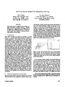
Figure 1: Our sequential and iterative parameter update procedure derived from the ADMM framework.

where ↵i and j represent Lagrange multipliers (or dual vari|U | |V| ables), and A = (↵i )i=1 and B = ( j )j=1 . Moreover, ⇢ is a tunable parameter to control the strength of constraint satisfaction during parameter estimation, where ⇢ > 0. Unfortunately, the joint optimization of Eq. (8) over all parameter sets is a hard problem. Thus, we leverage the ‘alternating direction method of multiplier (ADMM)’ algorithm [Gabay and Mercier, 1976; Boyd et al., 2011], as it provides an efficient optimization framework to solve problems in dual decomposition form like Eq. (8). The notable characteristic of ADMM is that it virtually decomposes the original optimization problem into several sub-problems, whose optimization variables are a (disjoint) subset of the original optimization variables. It sequentially and iteratively solves the sub-problems over the selected variable set while holding the other variables fixed. Detailed derivation for the general case can be found in [Boyd et al., 2011]. Fig. 1 shows our sequential and iterative parameter update procedure derived from the ADMM framework as applied to Eq. (8). Step1: If we discard all the terms that are independent from original optimization variables E and O, the objective function in Eq. (8) can be rewritten as follows: ⇢X ⇢X ||ei e0i ||22 + ||oj o0j ||22 , 1 = (E, O|D) + 2 i 2 j

be written as follows:

⇢ XX 0 ui,b 2 i b X X ⇢ 0 vj,b 2,V (V) = 2 j 2,U (U) =

ui,b

2 2

vj,b

2 , 2

(13)

b

0 = ei,b + ⇢1 ↵i,b and vj,b = P P 0 2 Note that i kui ui k2 = i

where o +1 , respecPj,b 0 ⇢ j,b 2 tively. ku u i,b k2 . i,b b We can further transform objective functions 2,U and 2,V in Eq. (13) by combining the parameter sharing constraints into the objective function. Finally, we obtain the following objective functions: n o ⇢ XX 2 0 min u0i,b pb,k 2 , 2,U (P) = k 2 i b n o XX (14) ⇢ 2 0 0 min vj,b qb,k 2 , 2,V (Q) = k 2 j u0i,b

b

as the replacements of 2,U and 2,V that include their constraints. Interestingly, both equations shown in Eq. (14) match the form of the objective function used as a standard k-means clustering problem. We can easily obtain a local optimum (or stationary point) by simply applying a standard k-means clustering algorithm. Step3: In the ADMM framework, dual variables are generally updated by one step of gradient ascent to tighten the constraints ei = ui and oj = vj , that is, ˆ i = ↵i + ⇠(ei ui ) 8i, ↵ (15) ˆj = j + ⇠(oj vj ) 8j, where ⇠ represents the learning rate of the gradient ascent method.

(12) where e0i = ui ⇢1 ↵i and o0j = vj ⇢1 j . Obviously, the minimization problem in Eq. (9) with 1 in Eq. (12) can be viewed as a conventional neural word embedding method with ‘shifted’ L2 -norm regularizers. Therefore, this optimization problem can be solved by gradient-based algorithms widely used in conventional neural word embedding methods, such as SGD or its variants. Step2: If we discard all the terms that are independent from auxiliary variables U, V, P and Q, we can further separate the sub-problem into two distinct parts (U, P) and (V, Q). Thus, the objective functions 2,U and 2,V in Eq. (10) can

4

Experiments

We followed the experimental settings used in a series of neural word embedding papers. First, our training data was

2049

Table 2: Benchmark datasets used in our experiments.

Table 4: Impact of dimension, D, for both performance and model size: (average performance of ten runs)

abbr. size OOV reference Word Similarity estimation (WordSim) MEN 3,000 0 [Bruni et al., 2014] MTurk 287 2 [Radinsky et al., 2011] RARE 2,034 313 [Luong et al., 2013] SLex 998 1 [Hill et al., 2014] SCWS 2,003 24 [Huang et al., 2012] WSR 252 14 [Agirre et al., 2009] WSS 203 7 [Agirre et al., 2009] Word Analogy estimation (Analogy) GSEM 8,869 0 [Mikolov et al., 2013a] GSYN 10,675 0 [Mikolov et al., 2013a] MSYN 8,000 0 [Mikolov et al., 2013c] Sentence Completion (SentComp) MSC 1,040 36 [Zweig and Burges, 2011]

method dimension model size WordSim Analogy SentComp SGNS D = 1024 3125MB 65.6 64.4 34.1 D = 512 1563MB 66.1 64.4 34.3 D = 256 781MB 64.0 63.5 32.7 D = 128 391MB 57.2 61.8 32.1 D = 64 195MB 44.4 59.5 30.1 D = 32 98MB 28.1 55.7 27.8

Table 5: Summary of our experimental results (average performance of ten runs); bold-type: better than ‘the worst performance in ten runs’ of SGNS. †GN100B shows the results of using a set of freely available pre-trained embedding vectors as briefly described in Sec. 1. Note that the learning configuration of GN100B is entirely different from SGSN and PS-SGNS. Thus, GN100B results are shown just for reference in confirming that our results are empirically valid.

Table 3: Hyper-parameters selected in our experiments and their candidate parameter sets.

parameter(s) for reducing model size (best in ten runs) (worst in ten runs) 16bit quant. 8bit quant. 4bit quant. 2bit quant. K = 256, B = 256 K = 16, B = 256 K = 256, B = 64 K = 16, B = 64 K = 16, B = 32 K = 256, B = 256 K = 16, B = 256 K = 256, B = 64 K = 16, B = 64 K = 16, B = 32 †GN100B (default:float 32bit) w/ quant. 16bit quant. post-proc. 8bit quant. 4bit quant.

hyper-parameter selected value candidate param. set context window (W ) 5 {2, 3, 5, 10} sub (t) † 10 5 (dirty) {0, 10 5 } cds (↵) † 3/4 {3/4, 1} post-process † e+o {e, o, e + o} initial learning rate (⌘) 0.025 {0.01, 0.025, 0.05} # of neg. sampling (k) 5 {1, 5, 10} # of iterations (T ) 10 {1, 2, 5, 10, 15}

method SGNS (D = 512) SGNS (D = 512) w/ quant. post-proc. SGNS w/ blockwise k-means post-proc. PS-SGNS (proposed method)

taken from a Wikipedia dump (Aug. 2014). We used the hyperwords tool6 for data preparation [Levy et al., 2015]. Finally, we obtained approximately 1.6 billion tokens of training data D. We selected 400,000 most frequent words in the training data as vocabularies of input and output words (|U| = |V| = 400, 000). Table 2 summarizes the benchmark datasets used in our experiments. We prepared three types of linguistic benchmark tasks: word similarity (WordSim), word analogy (Analogy), and sentence completion (SentComp). The ‘OOV’ column represents the number of words (problems) in each benchmark data that were out of vocabulary relative to our training data. Thus, these numbers also indicate the number of problems that are impossible to solve correctly in our experiments.

4.1

For a fair evaluation, we also examined two naive methods that can reduce the model size of embedding vectors.

Methods for comparing in our experiments

1. m-bit quantization: After obtaining the embedding vectors, we calculate the minimum and maximum values of every coordinate independently, and then evenly quantize the interval between minimum and maximum values into 2m -bins.

We selected SGNS as the baseline method since this is one of the most famous methods and is known to work well in many situations [Levy et al., 2015]. We used the word2vec implementation but modified the code to save the context vectors as well as the word vectors7 . Many tunable hyper-parameters were set based on the recommended default values or suggested values explained in [Levy et al., 2015]. Table 3 summarizes the hyper-parameters used consistently in all our experiments unless otherwise noted (See [Levy et al., 2015] for details of † in Table 3). Moreover, we selected ⇠ = 0.01, and ⇢ = 1.0 for hyper-parameters of our proposed method. 6 7

model Word- Ana- Sentsize Sim logy Comp 1565MB 67.2 64.7 35.9 1565MB 65.1 64.2 33.6 781MB 65.2 62.2 28.7 391MB 58.8 56.4 25.0 195MB 48.5 57.1 24.9 98MB 47.4 56.7 26.1 196MB 67.0 64.5 34.4 98MB 64.4 64.0 33.7 50MB 54.4 62.3 33.5 24MB 36.2 58.3 29.9 12MB 19.2 51.9 25.5 196MB 67.1 64.5 35.3 98MB 65.5 64.6 34.0 50MB 59.0 64.0 33.5 24MB 37.8 58.5 31.0 12MB 24.1 53.9 27.8 3433MB 73.6 65.5 38.0 1716MB 63.2 60.5 27.1 858MB 30.5 52.0 23.4 429MB 9.3 42.4 21.9

2. block-wise k-means clustering8 : We applied k-means clustering with exactly the same setting as the procedure of Step2 shown in Eq. (14). These two methods can be categorized as post-processing for model size reduction. 8 Note that simple vector-wise k-means clustering does not work for the purpose of model size reduction.

https://bitbucket.org/omerlevy/hyperwords https://code.google.com/p/word2vec/ (trunc42)

2050

Table 6: Detailed Results of Table 5; (average performance of ten runs)

parameters for model WordSim method reducing model size size MEN MTurK RARE SLex SCWS SGNS (default:float 32bit) 1565MB 77.1 69.5 48.4 65.7 39.2 PS-SGNS K = 256, B = 256 196MB 77.2 69.7 48.5 66.0 39.1 K = 16, B = 64 24MB 71.1 63.4 41.3 61.7 31.6 †GN100B (default:float 32bit) 3433MB 78.2 68.5 53.4 66.6 44.2

4.2

5

Task performance vs. model size

It is worth emphasizing here that our proposed method, which we refer to as ‘PS-SGNS’, is not intended to improve task performance. Our goal for PS-SGNS is to reduce the model size as much as possible while maintaining the task performance of the baseline method, SGNS.

WSR 66.0 65.7 59.6 63.5

Analogy WSS GSEM GSYN MSYN 78.7 79.7 63.7 51.0 79.1 80.6 64.8 51.6 73.7 48.4 37.6 23.0 77.2 73.1 74.0 73.6

SentComp dev. test 35.6 33.0 36.3 34.2 29.6 32.3 37.1 38.8

Related Work

Several papers have recently attempted to reduce the model size of neural networks in deep learning settings (NN/DL), i.e., [Droniou and Sigaud, 2013; Chen et al., 2015; Gupta et al., 2015; Courbariaux et al., 2015]. The motivation and purpose of our method are exactly the same as those studies. However, the methods developed for NN/DL cannot be directly or straightforwardly used in word embedding methods (like SGNS) in most cases. The first simple reason is that the target of most methods for NNs is to reduce the information of transformation matrices U in the transformation function o = f (Ue + b) since this part is generally the largest component of NNs. However, embedding methods like SGNS have no transformation matrices, U, in their models, namely, v = e · o. In addition, we emphasize that the problem for reducing the embedding vectors is much harder than that for NNs since the model capacity is already very limited. Moreover, the required properties are different. A simple example is provided by Analogy task. The embedding vectors are required to preserve the relation of angles and distances among all embedding vectors in the vector space. This basically is a very hard requirement. Based on these two reasons, our proposed method, PS-SGNS, seems to be much complicated compared to the methods used in NN/DL listed above. Our ADMM-based algorithm essentially is an extension of our previous study [Suzuki and Nagata, 2014]. However, there is an essential difference between them. The method introduced in this paper is realized by the fact that each dimension of embedding vectors has no interpretable meaning, and thus, exchangeable.

Baseline results with different model size (dimension) We first evaluated the impact of dimension D since it deeply affect to both performance and model size of our baseline method, SGNS. Table 4 shows the results. In our setting, D = 512 provided the best results. Thus, we selected ‘SGNS with D = 512’ as the base setting of our method, PS-SGNS. Comparison with original SGNS Table 5 summarizes our main results. Moreover, Table 6 shows results of individual benchmark datasets. PS-SGNS with ‘K = 16, B = 256’ had successfully reduces the model size nearly 16-fold compared to SGNS while generally matching SGNS task performance. In addition, the model size of PS-SGNS with ‘K = 16, B = 64’ was just 24MB, approximately 65 times smaller than that of original SGNS. Interestingly, the proposal still offered acceptable performance for WordSim and SentComp. Therefore, the embedding vectors obtained from PS-SGNS will be highly effective in applications running on limited memory devices. Analogy, on the other hand, seems to be very sensitive to model compaction. However, we emphasize that PS-SGNS provided significantly better results than all the baseline methods. In addition, we note that our method easily manage CBoW and similar word embedding method instead of SGNS as a baseline method. We omit to show PS-CBoW results since the tendency and relation of CBoW and PS-CBoW were essentially the same as SGNS and PS-SGNS.

6

Comparison with SGNS with block-wise k-means SGNS with the block-wise k-means post-processing method can be seen as a form of PS-SGNS. This is because SGNS with block-wise k-means post-processing essentially matches a single iteration of the ADMM-based algorithm shown in Fig. 1. Thus, comparing these two results roughly demonstrates the effectiveness of our method in terms of performing multiple iterations of ADMM updates. Obviously, multiple iterations significantly improved task performance. In addition, it is hard to prove that the proposed ADMM-based algorithm will converge to certain stationary point. This is because the original SGNS optimization problem is already a non-convex optimization problem. Therefore, these results provide empirical evidence that our ADMM-based algorithm has ability to find better solution by the iterative parameter update procedure.

Conclusion

This paper proposed a novel neural word embedding method that incorporates parameter sharing constraints during embedding vector learning. The embedding vectors obtained from our method strictly share the parameters in a certain predefined limited space. As a result, our method only needs to remember the set of shared parameters and selection information for recovering completely all embedding vectors; our approach can significantly reduce the model size. This paper also introduced an efficient learning algorithm based on the ADMM framework for solving the optimization problem with our parameter sharing constraints. Our experiments showed that SGNS with our parameter sharing constraints, which we call PS-SGNS, successfully reduced the model size by more than one order of magnitude while matching the task performance of the original SGNS.

2051

References

[Levy et al., 2015] Omer Levy, Yoav Goldberg, and Ido Dagan. Improving Distributional Similarity with Lessons Learned from Word Embeddings. Transactions of the ACL, 3, 2015. [Liu et al., 2014] Shujie Liu, Nan Yang, Mu Li, and Ming Zhou. A Recursive Recurrent Neural Network for Statistical Machine Translation. In Proc. of the 52nd Annual Meeting of the ACL, 2014. [Luong et al., 2013] Thang Luong, Richard Socher, and Christopher Manning. Better Word Representations with Recursive Neural Networks for Morphology. In Proc. of the Seventeenth Conference on CoNLL, pages 104–113, 2013. [Mikolov et al., 2013a] Tomas Mikolov, Kai Chen, Greg Corrado, and Jeffrey Dean. Efficient Estimation of Word Representations in Vector Space. CoRR, abs/1301.3781, 2013. [Mikolov et al., 2013b] Tomas Mikolov, Ilya Sutskever, Kai Chen, Greg S Corrado, and Jeff Dean. Distributed Representations of Words and Phrases and their Compositionality. In Advances in Neural Information Processing Systems 26, pages 3111–3119. Curran Associates, Inc., 2013. [Mikolov et al., 2013c] Tomas Mikolov, Wen-tau Yih, and Geoffrey Zweig. Linguistic Regularities in Continuous Space Word Representations. In Proc. of the 2013 Conference of the NAACL: Human Language Technologies, pages 746–751, 2013. [Miller and Charles, 1991] George A. Miller and Walter G. Charles. Contextual Correlates of Semantic Similarity. Language & Cognitive Processes, 6(1):1–28, 1991. [Mnih and Kavukcuoglu, 2013] Andriy Mnih and Koray Kavukcuoglu. Learning Word Embeddings Efficiently With Noise-contrastive Estimation. In Advances in Neural Information Processing Systems 26, pages 2265–2273. Curran Associates, Inc., 2013. [Pennington et al., 2014] Jeffrey Pennington, Richard Socher, and Christopher Manning. Glove: Global Vectors for Word Representation. In Proc. of the 2014 Conference on EMNLP, pages 1532–1543, 2014. [Powell, 1969] M. J. D. Powell. A method for nonlinear constraints in minimization problems. In Optimization, pages 283–298. Academic Press, 1969. [Radinsky et al., 2011] Kira Radinsky, Eugene Agichtein, Evgeniy Gabrilovich, and Shaul Markovitch. A Word at a Time: Computing Word Relatedness Using Temporal Semantic Analysis. In Proc. of the 20th International Conference on WWW, pages 337– 346, 2011. [Suzuki and Nagata, 2014] Jun Suzuki and Masaaki Nagata. Fused Feature Representation Discovery for High-dimensional and Sparse Data. In Proc. of the Twenty-Eighth AAAI Conference on Artificial Intelligence, pages 1593–1599, 2014. [Suzuki and Nagata, 2015] Jun Suzuki and Masaaki Nagata. A Unified Learning Framework of Skip-Grams and Global Vectors. In Proc. of the 53rd Annual Meeting of the ACL and the 7th IJCNLP, pages 186–191, 2015. [Turian et al., 2010] Joseph Turian, Lev-Arie Ratinov, and Yoshua Bengio. Word Representations: A Simple and General Method for Semi-Supervised Learning. In Proc. of the 48th Annual Meeting of the ACL, pages 384–394, 2010. [Zweig and Burges, 2011] Geoffrey Zweig and Christopher J.C. Burges. The Microsoft Research Sentence Completion Challenge. Technical Report MSR-TR-2011-129, Microsoft Research, 2011.

[Agirre et al., 2009] Eneko Agirre, Enrique Alfonseca, Keith Hall, Jana Kravalova, Marius Pas¸ca, and Aitor Soroa. A Study on Similarity and Relatedness Using Distributional and WordNet-based Approaches. In Proc. of Human Language Technologies: The 2009 Annual Conference of the NAACL, pages 19–27, 2009. [Boyd et al., 2011] Stephen Boyd, Neal Parikh, Eric Chu, Borja Peleato, and Jonathan Eckstein. Distributed Optimization and Statistical Learning via the Alternating Direction Method of Multipliers. Foundations and Trends in Machine Learning, 2011. [Bruni et al., 2014] Elia Bruni, Nam Khanh Tran, and Marco Baroni. Multimodal distributional semantics. J. Artif. Int. Res., 49(1):1–47, 2014. [Chen and Manning, 2014] Danqi Chen and Christopher Manning. A Fast and Accurate Dependency Parser using Neural Networks. In Proc of the 2014 Conference on EMNLP, pages 740–750, 2014. [Chen et al., 2015] Wenlin Chen, James Wilson, Stephen Tyree, Kilian Q. Weinberger, and Yixin Chen. Compressing neural networks with the hashing trick. In Proc. of the 32nd ICML, pages 2285–2294, 2015. [Courbariaux et al., 2015] Matthieu Courbariaux, Yoshua Bengio, and Jean-Pierre David. Binaryconnect: Training deep neural networks with binary weights during propagations. In Advances in Neural Information Processing Systems 28, pages 3105–3113. Curran Associates, Inc., 2015. [Droniou and Sigaud, 2013] Alain Droniou and Olivier Sigaud. Gated Autoencoders with Tied Input Weights. In Proc. of the 30th ICML, pages 154–162, 2013. [Everett, 1963] Hugh Everett. Generalized Lagrange Multiplier Method for Solving Problems of Optimum Allocation of Resources. Operations Research, 11(3):399–417, 1963. [Gabay and Mercier, 1976] D. Gabay and B. Mercier. A Dual Algorithm for the Solution of Nonlinear Variational Problems via Finite-Element Approximations. Computer Math. Applications, 2:17–40, 1976. [Guo et al., 2014] Jiang Guo, Wanxiang Che, Haifeng Wang, and Ting Liu. Revisiting Embedding Features for Simple Semisupervised Learning. In Proc. of the 2014 Conference on EMNLP, pages 110–120, 2014. [Gupta et al., 2015] Suyog Gupta, Ankur Agrawal, Kailash Gopalakrishnan, and Pritish Narayanan. Deep Learning with Limited Numerical Precision. In Proc. of the 32nd ICML, pages 1737–1746, 2015. [Hestenes, 1969] Magnus R. Hestenes. Multiplier and gradient methods. Journal of Optimization Theory and Applications, 4(5):303–320, 1969. [Hill et al., 2014] F. Hill, R. Reichart, and A. Korhonen. SimLex999: Evaluating Semantic Models with (Genuine) Similarity Estimation. ArXiv e-prints, 2014. [Hinton and Salakhutdinov, 2012] Geoffrey E. Hinton and Ruslan R Salakhutdinov. A Better Way to Pretrain Deep Boltzmann Machines. In Advances in Neural Information Processing Systems 25, pages 2447–2455. Curran Associates, Inc., 2012. [Huang et al., 2012] Eric H. Huang, Richard Socher, Christopher D. Manning, and Andrew Y. Ng. Improving Word Representations via Global Context and Multiple Word Prototypes. In Proc. of the 50th Annual Meeting of the ACL, pages 873–882, 2012.

2052