Sep 8, 2013 - shows the latest advances in the project Statistics-to-Go. Finally, Section VI presents ... Android is an operating system designed primarily for.
PAPER LEARNING CONFIDENCE INTERVALS WITH MOBILE DEVICES
Learning Confidence Intervals with Mobile Devices http://dx.doi.org/10.3991/ijim.v7i4.2788
F.J. Tapia-Moreno, H.A.Villa-Martinez University of Sonora, Hermosillo, México
Abstract— Mobile learning (m-learning) enhances learning skills in some students. Mobile phones, Tablets, PDAs, Pocket PCs, and Internet can be used jointly in order to encourage and motivate learning wherever and whenever students want to learn. In this work, we show learning objects for teaching and learning inferential statistics using mobile devices. With these learning objects, students can calculate confidence intervals based in either a large or a small data sample obtained from a normal or a non-normal population. These objects have been designed for devices with Android operating system. Index Terms—m-learning, inferential statistics, learning objects.
I.
INTRODUCTION
In April of 2012 we presented a paper about the main results obtained in the project Statistics-to-Go [1] in which we developed learning objects for descriptive statistics by means of three Java-ME suites named Module 1, Visual Summary Measures, and Skewness Measures. We wrote the corresponding user manuals. These learning objects are currently used by the students who take the statistics courses offered in the University of Sonora. The success in the use of these learning objects has motivated us to build a module for inferential statistics. In this paper, we present learning objects for calculate confidence intervals based in either a large or a small sample of data obtained from a normal or a non-normal population. The remainder of this paper is composed as follows: Section II presents a short review about the state of art in mobile learning. Section III shows details about Android operating system and what can be created on mobile devices which use this operating system. Section IV presents basic confidence intervals theory. Section V shows the latest advances in the project Statistics-to-Go. Finally, Section VI presents our conclusions and future work. II.
MOBILE LEARNING
Mobile learning (also known as m-learning) is the acquisition of knowledge by means of some mobile device, for example a cellular phone or a tablet computer [2]. m-learning is extremely effective in classroom environments where modern technology may not be available to all students, or in schools where there are not sufficient computational resources for all students. In such situations, using a mobile device for learning, a device that can be shared among a group of students, is a great
4
way to ensure that pupils are still able to benefit from the diverse opportunities presented by educational technology. Some of the reported uses of m-learning are: to enhance the user experience in visitors of an art museum, to take advantage of the learning context [3], to allow students to participate on an academic discussion forum [4], in training for personnel in disaster or emergency situations [5], to suggest didactic methods that are adequate to a specific teaching situation [6], and in the learning of science [7], languages [8], and medicine [9]. The differences between m-learning and other types of learning can be studied by considering both the technology involved and the educational experience. Regarding technology, m-learning differs in the use of portable equipment that allows students to access learning objects anytime and anywhere. Regarding the educational experience, Traxler [10] compares m-learning and traditional e-learning using keywords. This way, mlearning is “personal”, “spontaneous”, “opportunistic”, “informal”, “pervasive”, “private”, “context-aware”, “bite-sized”, and “portable”, whereas e-learning is “structured”, “media-rich”, “broadband”, “interactive”, “intelligent”, and “usable”. The same author notes that some of these distinctions can disappear as mobile technology advance, but properties as informality, mobility, and context will remain. III.
ANDROID OPERATING SYSTEM
Android is an operating system designed primarily for mobile devices such as cellular phones and tablet computers. Initially developed by Android, Inc., which Google bought in 2005, Android was unveiled in 2007 along with the founding of the Open Handset Alliance, a consortium of hardware, software, and telecommunication companies devoted to advancing open standards for mobile devices. The first Android-powered phone was sold in October 2008 [11]. Android-based cellular phones lead the market. According to Tech-Thoughts [12], Android has a share of almost 70% in the global smartphone market, while iOS, made by Apple, accounts to about 14%. In fact, Android has the largest share in every developed country, except in the United States and Japan where iOS is the dominant mobile operating system [13, 14]. In the tablet world the story is similar. According to BGR [15], Android worldwide market share grew from 39.8% in 2011 to 42.7% in 2012, while iOS share diminished from 56.3% to 53.8%.
http://www.i-jim.org
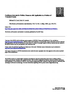
PAPER LEARNING CONFIDENCE INTERVALS WITH MOBILE DEVICES IV. CONFIDENCE INTERVALS In statistical inference, one wishes to estimate population parameters (for example average, variance, standard deviation, proportions, and differences between means and/or proportions) using observed sample data. A confidence interval gives an estimated range of values which is likely to include the unknown population parameter. This estimated range is calculated from a given set of sample data. Each confidence interval has associated a measure of the certainty that the interval confidence contains the population’s parameter. This measure is called confidence level and is indicated by 1!!, where !, a number between 0 and 1, is called the significance grade. The most used confidence levels are 90%, 95%, and 99%. Each one of these numbers represents the probability that the confidence interval contains the real valor of the population parameter. Figure 1 shows a confidence interval for the population’s average ! based in an observed sample data. !! is the sample’s average.
!!!!
According to Triola [16], from a population sample a confidence interval can be constructed for the population’s mean using the normal distribution when: 1) the size of the sample is larger than 30 (! ! !") (this is due to the central limit theorem), or 2) when the sample size is less than 30 (! ! !"!, but the population has a normal distribution and its standard deviation is known. For this case, the confidence interval is given by Equation (1). ! !!!!!!!! ! ! !!!!!! ! !
Note that if the population’s standard deviation is unknown, then Equation (2) should be used for determining the confidence interval. !
!
(2)
where ! is the sample’s mean, ! is the sample’s standard deviation, ! is the size of the sample, and !!!!!! is the critical value of the normal standardized distribution [16]. If the size of the sample is less than 30 (! ! !"!, the population a has normal distribution, and the standard deviation is unknown, then the Student’s distribution is preferred for constructing the confidence interval for population’s mean [2]. In this case, the confidence interval is given by Equation (3) ! !!!!!!!!! ! ! !!!!!!!!!! ! !
iJIM ‒ Volume 7, Issue 4, October 2013
!
!!!!!!!!! ! where ! ! !!!.
In a similar way, confidence intervals for a population’s proportion can be build using the normal distribution as an approximation to the binomial distribution if ! ! !"!!and either ! ! ! ! ! or ! ! !! ! !! ! !. Here, ! is the sample size and ! is the probability of success in the experiment [16]. The confidence interval for this case is presented in Equation (6).
where
Figure 1.
! ! !!!!!! !
where ! is the sample’s mean, ! is the sample’s standard deviation, ! is the size of the sample, ! ! ! are the degrees of freedom, and !!!!!!!!!! is the corresponding critical value for the confidence grade (! ! !!!) of the Student’s distribution. When the size of the sample is less than 30 (! ! !") and the population has a non-normal distribution, then the Chebyshev’s Theorem can be used to build a confidence interval for the population’s mean [16]. Equations (4) and (5) show the confidence interval for this case when the population’s standard deviation is known and unknown, respectively. ! !!!!!!!!! !!!! !
!! !
! ! !!!!!! ! !! !!!!!!!
!!!!!!! !
!!!!or
!! !
!!!!!!! !
!
!!!
if
!!!
! ! !!!" ! !. Here ! is the population size, and ! is the probability of success in the experiment. Similarly, confidence intervals can be constructed for the difference between the means of two populations and for the difference between the proportions of two populations. The confidence interval for each one of these cases is shown in Equations (7), (8), (9), (10), (11), and (12). !! ! !! ! !!!!!! ! !!!!!! !!!!!! !! ! !! ! !!!!!! ! !!!!!! !!!!!!
!! ! !! ! !!!!!!!!!!!!!!!! ! !!!!!! !!!!!! !! ! !! ! ! ! !!!!!! !!!!!"! !! ! !! ! ! ! !!!!!! !!!!!!!
!! ! !! ! !!!!!! ! !!!!!! !!!!!"! where !!!!!! !
!!!!!! ! !! ! !!!! !!
!!! !!
!
!
!!! !!
;
!! ! !!!! !!
!!!!!! !
!!!
!!
!
!!!
!!
;
, and !! , !! , !! , !! , !! ,
!! , !! ! !! ! !! , and !! are respectively, the means, standard deviations of the populations, standard deviations
5
PAPER LEARNING CONFIDENCE INTERVALS WITH MOBILE DEVICES of the samples, proportions of the samples, and the samples sizes. If a sample is taken from a normal distribution, confidence intervals can be built for both population’s variance and standard deviation using the chi square distribution [17]. Both confidence intervals are given in Equations (13) and (14), respectively. ! ! ! ! !! ! ! ! ! !! ! ! ! ! !!!!!!!"! ! ! !!!!!!!!!""#$ !!!!!!!!!"#$% ! ! ! ! !! !!! ! !!!!!!!!!""#$
The second object computes confidence intervals for the population’s average when the size of the sample is less than 30 (! ! !"), the population has a normal distribution, and the standard deviation is unknown. For this case, the Student’s distribution is the preferred way for constructing the confidence interval for the population’s mean. In this case, the system uses Equation (3) in order to calculate it. Figure 3 shows the output of this object for a sample with size ! ! !", a mean of 7.5, a standard deviation of 2.1, and a confidence level of 95%.
! ! ! ! !! !!!!!!!"! ! !!!!!!!!!"#
%$where the upper and lower sub-indices identify the percentiles points of the chi-square distribution that was used for constructing the confidence interval. Finally, we can build confidence interval for the ratio of variances of two normally distributed populations using the F distribution [16] employing Equation (15). !!! !!!!
!!!!!!
!
!!! !!!
!
!!! !!!! !!!!
(15)
One last remark is that a person who wants to calculate confidence intervals needs statistics tables, like those in [17], in order to obtain the proportion of the area under the normal curve, the Student t, the chi-square, and the F factor. On the other hand, our system obviates this requirement. IV. RESULTS In this second stage of our project, we have developed learning and teaching objects for Inferential Statistics. Each one of the objects calculates a confidence interval for a distinct situation. The first object computes confidence intervals for the population’s mean. The application uses Equations (1) or Equation (2) depending if the value of the population’s standard deviation is known or not. Figure 2 shows the output of this object for a sample with size ! ! !", a mean of 7.5, a standard deviation of 2.1, and a confidence level of 95%. That is, ! ! !!!"!
Figure 3.
The third object computes confidence intervals for the population’s average when the population has a nonnormal distribution. The Chebyshev’s theorem is used to build this confidence interval. The application uses Equation (4) or Equation (5) depending if the value of the population’s standard deviation is known or not. Figure 4 shows the output of this object for a sample with ! ! !", a mean of 7.5, a standard deviation of 2.1, and a confidence level of 95%.
Figure 4.
The fourth object calculates confidence intervals for a population’s proportion using Equation (6). This application can be used only when both conditions mentioned in section IV are satisfied. Figure 5 presents the output of this object for a population with size ! ! !"", and a sample of size ! ! !" with a proportion of ! ! !!!" and a confidence level of 95%. Figure 2.
6
http://www.i-jim.org
PAPER LEARNING CONFIDENCE INTERVALS WITH MOBILE DEVICES
Figure 5.
The fifth object computes confidence intervals for the difference between the means of two populations using Equation (7) or Equation (8) depending if both population’s standard deviations are known or not. Figure 6 shows the output of this object for two samples with sizes !! ! !" and !! ! !!, sample’s means of !! ! !"!!" and !! ! !!!!, and sample’s standard deviations of !! ! !!! and !! ! !!!"#, with confidence level of 95%.
Figure 7.
The ninth object computes confidence intervals for the population’s variance and standard deviation using the chi square distribution. The object uses Equation (13) or Equation (14) to estimate these confidence intervals. Figure 8 shows the result output for a sample with size ! ! !", a standard deviation of 7.5, and a confidence level of 95%.
Figure 8. Figure 6.
The sixth object computes confidence intervals for the difference between the means of two populations when both two samples are little (!! ! !!