Feb 26, 1997 - ant language classes (including the regular and context-free ones) cannot be ... Learning context-free languages is harder, but recently some ...
Learning context-free grammars from stochastic structural information� Rafael C. Carrasco and Jose Oncina Departamento de Lenguajes y Sistemas Inform�aticos Universidad de Alicante, E-03071 Alicante E-mail: (carrasco, joncina)@dlsi.ua.es February 26, 1997 Abstract
We consider the problem of learning context-free grammars from stochastic structural data. For this purpose, we have developed an algorithm (tlips) which identi es any rational tree set from stochastic samples and approximates the probability distribution of the trees in the language. The procedure identi es equivalent subtrees in the sample and outputs the hypothesis in linear time with the number of examples.
Running title Learning CF stochastic grammars Keywords stochastic languages, machine learning, language identi cation AMS subject 68Q75
� Work
partially supported by the Spanish CICYT under grant TIC93-0633-C02
1
1 Introduction Grammatical inference is the task of learning a correct grammar for a language from examples. Gold (1967) introduced the criterion of identi cation in the limit for successful learning of a language, and also showed that many relevant language classes (including the regular and context-free ones) cannot be learned from positive samples1, essentially due to the problem of overgeneralization. One way to avoid this problem is to provide complete samples. A complete sample presents all strings as belonging or not to the language. In practice, complete samples are scarce, as they mean a complete knowledge of the language. An alternative way to overcome overgeneralization is the use of stochastic samples, something closer to most experimental scenarios where random or noisy examples appear. Angluin (1988) proved that identi cation in the limit is possible from stochastic samples provided that rather general assumptions about the probability distribution are made. This general result explains the success in nding algorithms which identify regular languages from positive stochastic data. Indeed, algorithms working in polynomial time have been proposed by Stolcke and Omohundro (1993) and by Carrasco and Oncina (1994). Learning context-free languages is harder, but recently some interesting results have been found. Sakakibara (1992) addressed the related problem of learning context-free grammars from positive examples of their structural descriptions. Structural descriptions of context-free languages may appear, for instance, when examples of strings in the language are presented in bracketed form. Every set of structural descriptions is a rational set of trees (i.e., a set which can be recognized by a tree automaton). Therefore, the identi cation problem can be reduced to that of learning rational tree languages. In that work (Sakakibara, 1992), he proves that the subclass of reversible tree languages can be learned in polynomial time from positive examples. Reversible tree languages are the extension of the reversible regular languages studied by Angluin (1982), and are properly included in the class of rational tree languages2 . Indeed, the class of rational tree sets is not identi able in the limit from positive data. A more general algorithm has been recently proposed by Oncina and Garc��a (1994). Their algorithm identi es any rational tree language, works in polynomial time and uses both positive and negative examples during the training process. Because this last property restricts its applicability, we present in this paper a new algorithm which can be trained with positive stochastic samples generated according to a probabilistic production scheme. Once the rational language of derivation trees is identi ed, there is always a backwards deterministic (Aho and Ullman, 1972) form of the context-free grammar compatible with the set of derivation trees, and the probability distribution can be approximated with any desired accuracy, provided that enough examples are given. Our notation follows closely that of Sakakibara (1992) and is described in Section 2, before the algorithm is presented in Section 3. The probabilistic version is introduced in Section 4 and an experimental example is presented in Section 5. Finally, conclusions are drawn in Section 6. 1 2
A positive sample presents all and only examples from the target language. Even if reversibility can be considered a normal form for context-free grammars.
2
2 Preliminaries
Let N be the set of natural numbers and N� be the free monoid generated by N with \." as the operation and � as the identity. The length of x 2 N� is denoted as jxj, and satis es j�j = 0 and jx:yj = jxj + jyj for all x; y 2 N�. A subset D � N� is a tree domain if for all x; y 2 N� and for all i; j 2 N x:y 2 D ) x 2 D (1) x:i 2 D ^ j � i ) x:j 2 D A ranked alphabet V is a nite set of symbols with a nite relation (called rank): r � (V � N). The elements in V of rank k are Vk = ff 2 V : (f; k) 2 rg. Note that the sets Vk are not necessarily disjoint. A nite tree over a ranked alphabet V is a mapping t : dom(t) ! V where dom(t) is a nite tree domain such that t(x) 2 Vk with k = minfi 2 N : x:i 62 dom(t)g. The depth of a tree is the maximum length of the elements in its domain: depth(t) = maxfjxj : x 2 dom(t)g: (2) The set of nite trees over V will be denoted with V T . The alphabet V can be regarded as a set of function symbols whose rank is the function arity. In the following, trees will be written in the form t = f(t1 ; :::; tk), where f is a symbol in Vk . Note that V0 coincides with the subset of trees in V T whose domain is �. Let V be a ranked alphabet and n the greatest rank of the symbols in V . A deterministic tree automaton (DTA) is de ned as A = (Q; V; �; F), where Q is a nite set of states, F � Q is the subset of accepting states, and � = (�0 ; : : :; �n) is a n-tuple of functions with the form �k : Vk � Qk ! Q: (3) The DTA operates on trees as follows: � (f; �(t1); : : :; �(tk )) if t = f(t1 ; : : :; tk ) 2 V T ? V0 (4) �(t) = ��0k(t) if t 2 V0 Every DTA de nes a rational tree language (RTL): L(A) = ft 2 V T : �(t) 2 F g (5) For every �-production free (Hopcroft, 1979) context-free grammar G = (N; �; P; S), we (recursively) de ne the set of trees rooted at X 2 (N [ �) as: 8 if X 2 � < fX g DX (G) = : fX(t1 ; :::; tn) : X ! X1 :::Xn 2 P ^ (6) ^ ti 2 DX (G); 1 � i � ng if X 2 N The trees in DS (G) are also called derivation trees of G. For every t 2 V T , the skeleton of t can be de ned as: � 0 sk(t) = t�(sk(t ); : : :; sk(t )) ifif tt 2= Vf(t (7) T ? V0 ) 1 k 1 ; : : :; tk ) 2 (V where � is a special symbol whose arities are all strictly positive. Internal nodes in the skeleton are labeled with �, while leaves are labeled with symbols in �. i
3
Both the set of derivation trees DS (G) and the set of their skeletons sk(DS (G)) are rational tree sets. For instance, given a backwards-deterministic grammar G = (N; �; P; S), it is possible to de ne the acceptor (Q; V; �; F) with Q V �0 (a) �k (�; X1; :::; Xk)
N [� f�g [ �
= = = =
a A
8a 2 � if A ! X1 :::Xk 2 P
(8)
which recognizes sk(DS (G)). It is also straightforward to obtain a (backwards deterministic) grammar generating the skeletal language de ned by this DTA. A stochastic tree language T is de ned by a probability density function over V T denoted as p(tjT). The probability of any subset S � V T is p(S jT) =
X
t2S
p(tjT):
(9)
On the other hand, two stochastic languages are identical if T1 = T2 , p(tjT1 ) = p(tjT2 ) 8t 2 V T :
(10)
A stochastic DTA, A = (Q; V; �; r; p), incorporates the probability r : Q ! [0; 1] that a node appears at the root of a tree X
q2Q
r(q) = 1
(11)
plus a set of probability functions p = (p0; : : :; pn) of the form pk : Vk � Qk ! [0; 1], such that for all qi 2 Q 1=
n
X X
X
k=1 f 2Vk q1 ;:::qk 2Q
pk (f; q1; :::; qk)
(12) �(f;q1 ;:::qk )=qi
A stochastic rational tree language can be de ned through the density function p(tjA) = r(�(t))p(t) (13) where the probability of the tree t = f(t1 ; ::; tk) is p(t) = pk (f; t1 ; :::; tk)p(t1) � � � p(tk ):
(14)
Let $ 62 V be a new symbol of rank zero. With V$T we denote the set of trees in (V [ f$g)T containing exactly one symbol $. For every s 2 V$T , and every t 2 (V T [ V$T ), the $-replacement s#t is de ned by � s(x) if x 2 dom(s) ^ s(x) 6= $ s#t(x) = t(z) (15) if x = y:z ^ s(y) = $ and x 62 dom(s#t) otherwise. 4
For every stochastic tree language T and t 2 V T , the quotient t?1 T is a stochastic language over V$T de ned through the probabilities
jT) : p(sjt?1 T) = p(s#t (16) p(V$T #tjT) In case s 62 V$T then p(sjt?1T) = 0. On the other hand, if p(V$T #tjT) = 0, the quotient (16) is unde ned and we will write t?1T = ;. The Myhill-Nerode's theorem for rational languages (see for instance, Hopcroft 1979) can be generalized for stochastic rational tree languages. If T is a stochastic RTL, then the number of di�erent sets t?1T is nite and a deterministic tree automaton (DTA) accepting ft 2 V T : p(tjT) > 0g can be de ned. We will call it the canonical acceptor M = (QM ; V; � M ; F M ), with:
QM = ft?1T 6= ; : t 2 V T g F M = ft?1T : p(tjT) > 0g (17) ? 1 ? M � (f; t1 T; : : :; tk 1T) = f(t1 ; : : :; tk )?1 T A stochastic sample S of the language T is an in nite sequence of trees generated according to the probability distribution p(tjT). We denote with Sn the sequence of the n rst trees (not necessarily di�erent) in S andPwith cn (t) the number of occurrences of tree t in Sn . For X � V T , cn(X) = t2X cn(t). Provided that the structure (states and transition functions) of M is known, we can estimate the probability functions in the stochastic DTA from the examples in Sn : t) (18) r(t?1T) = cn(� n cn (V$T #t) pk (f; t?1 1 T; : : :; t?k 1T) = (19) cn(V$T #�t) : where �t = fs 2 V T : � M (s) = t?1 T). The accuracy of these estimates improves with n. In the following section we present an algorithm identifying the structure of the automaton M.
3 Inference algorithm In the following, we will assume that an arbitrary total order relation has been de ned in V T such that t1 � t2 , depth(t1 ) � depth(t2 ). As usual, t1 < t2 , t1 � t2 ^ t1 6= t2. The subtree set and the short-subtree set are respectively de ned as Sub(T) = ft 2 V T : t?1 T 6= ;g (20) SSub(T) = ft 2 Sub(T) : s?1 T = t?1T ) s � tg The kernel and the frontier set are de ned as: K(T) = ff(t1 ; :::; tk) 2 Sub(T) : t1 ; :::; tk 2 SSub(T)g (21) F(T) = K(T) ? SSub(T) 5
algorithm tlips input: output:
A � Sub(T) such that K(T) � A SSub (short subtree set) F (frontier set)
begin algorithm
SSub = F = ; W = V0 \ A do ( while W 6= ; ) x = minW W = W ? fxg if 9y 2 SSub : equivT(x; y) then F = F [ fxg else
SSub = SSub [ fxg W = W [ ff(t1 ; :::; tk) 2 A : t1 ; :::; tk 2 SSubg
endif end do end algorithm
Figure 1: Algorithm tlips. Note that there is exactly one tree in SSub(T) for every state in QM of the canonical acceptor, while the trees in K(T) ? V0 correspond to the rules in the generating grammar and, therefore, both SSub(T) and K(T) are nite. Let us de ne a boolean function equivT : K(T) � K(T) ! ftrue; falseg such that 1 ?1 equivT(t1 ; t2) = true , t? (22) 1 T = t2 T: We will make use of the following lemma: Lemma 1 If SSub(T), F(T) and equivT are known, then the structure of the
canonical acceptor is isomorphic to:
Q = SSub(T) �(f; t1 ; :::; tk) = t where t is the only tree in SSub(T) such that equivT(t; f(t1 ; :::; tk))
(23)
Proof. Let � be a mapping that for every language t?1 T gives the only tree s = �(t?1 T) in SSub(T) such that s?1 T = t?1T. Clearly, if t 2 SSub(T) then �(t?1 T) = t. The mapping � is an isomorphism if �(f; �(t?1 1 T); :::; �(t?k 1T)) = �� M (f; t?1 1T; :::; t?k 1T): As t1; :::; tk are in SSub(T), and � M (f; t?1 1T; :::; t?k 1T) = f(t1 ; :::; tk)?1 T, then one can rewrite the above condition as �(f; t1; :::; tk) = �(f(t1 ; :::; tk)?1T) which holds if �(f; t1; :::; tk) is the only tree t 2 SSub(T) satisfying t?1T = f(t1 ; :::; tk)?1 T. Note that t1 ; :::; tk 2 SSub(T) implies f(t1 ; :::; tk) 2 K(T), and therefore, the condition can be written as equivT(t; f(t1 ; :::; tk)). Next theorem supports the inference algorithm. Theorem 2 The algorithm in Fig. 1 outputs SSub(T) and F(T) with input equivT plus any A � Sub(T) such that K(T) � A. 6
algorithm compn T n input: output: begin algorithm do if different
x; y 2 V ; S boolean
( 8t; z : depth(t) = 1 ^ (t#z#x _ t#z#y) 2 Sub(Sn ) ) (cn (V$T #t#z#x); cn(V$T #x); cn(V$T #t#z#y); cn(V$T #y); �) then
return endif end do return true end algorithm
false
Figure 2: Algorithm compn. Proof.(sketch) Induction shows that after i iterations SSub[i] � SSub(T), F [i] � F(T) and W [i] � K(T). On the other hand, if t 2 K(T) then t 2 A and induction in the depth of the tree shows that t eventually enters the algorithm. For instance, the set Sub(Sn ) � Sub(T) can be used as input in the former algorithm, as K(T) � Sub(Sn ) for n large enough. On the other hand, the algorithm never calls equivT out of its domain K(T) and the number of calls is bounded by jK(T)j2 . Thus, the global complexity of the algorithm is O(jK(T)j2 ) times the complexity of function equivT.
4 Probabilistic inference In practice, the unknown language T is replaced by the stochastic sample S and the equivalence test equivT(x; y) is performed through a probabilistic function compn(x; y) of the n rst trees in S (i.e., of Sn ). The algorithm will output the correct DTA in the limit as long as compn tends to equivT when n grows. According to (22), equivT(x; y) = true means x?1T = y?1 T. This can be checked by means of eq. (16), but we rather check the conditional probabilities: p(V$T #t#z#x) p(V$T #t#z#y) p(V$T #z#x) = p(V$T #z#y)
(24)
for all z 2 V$T and for all t 2 V$T with depth(t) = 1. In order to check (24) a statistical test is applied to the di�erence (provided that t#z#x or t#z#y are in Sub(Sn )): cn(V$T #t#z#x) cn(V$T #t#z#y) cn(V$T #z#x) ? cn (V$T #z#y) ;
(25)
where cn counts the number of occurrences in Sn of the trees in the argument. We have chosen a Hoe�ding (1963) type test, as described in the Appendix. This check provides the correct answer with probability greater than (1 ? �)2 , being � an arbitrarily small positive number. Therefore, the algorithm compn plotted 7
in Fig. 2 returns the correct value with probability greater than (1 ? �)2r , where r is smaller than the number of di�erent subtrees in Sn . Because r grows slowly with n, we allow � to depend on r. Indeed, if � decreases faster than 1=r then (1 ? �)r tends to zero and compn(x; y) = equivT(x; y) in the limit of large n. Finally, note that the complexity of compn is at most O(n). As jK(T)j does not depend on Sn then the global complexity of our algorithm is O(n).
5 An example The following probabilistic context-free grammar generates conditional statements: statement ! if expression then statement else statement endif (0.2) statement ! if expression then statement endif (0.4) statement ! print expression (0.4) expression ! expression operator term (0.5) expression ! term (0.5) term ! number (1.0) where variables appear in italics, terminals in bold and the number in parenthesis represents the probability of the rule. The average number of rules in the hypothesis as a function of the number of examples is plotted in Fig. 3. When the sample is small, rather small grammars are found and overgeneralization occurs. As the number of examples grows, the algorithm tends to output a grammar with the correct size, and for larger samples (above 150 examples) the correct grammar is always found. Similar behavior was observed for other grammars and experiments. On the other hand, our implementation needed about 15 seconds (running on a Hewlett-Packard 715 with 40 MIPS) for a 1000 trees sample of this language.
6 Conclusions The algorithm tlips learns context-free grammars from stochastic examples of parse tree skeletons. The result is, in the limit, structurally identical to the target grammar (i.e., they generate the same stochastic set of skeletons) and is found in linear time with the size of the sample. Experimentally, identi cation is reached with relatively small samples and the algorithm proves fast enough for application purposes. We are presently working on adapting this algorithm for the inference of graph grammars in character recognition.
Acknowledgments We thank M.L. Forcada his useful suggestions while writing the manuscript.
8
8 7 6 5 4
�
3
� �
� � �
20
40
� �
� � � � � � � �
2 1 0
0
60
80 100 size of sample
120
140
160
Figure 3: Number of rules in the hypothesis as a function of the number of examples. The target grammar has 6 rules.
A Appendix We will use the following bound (Hoe�ding 1963) for the observed frequency f=m of a Bernoulli variable of probability p. Let � > 0 and let r
1 log 2 �� (m) = 2m � then, with probability greater than 1 ? �, f < � (m) p ? m � It follows immediately that, with probability greater than (1 ? �)2,
f m
? mf < ��(m) + ��(m0 ) if
f m
? mf > ��(m) + ��(m0 ) if jp ? p0j > 2(�� (m) + �� (m0 ))
0
p = p0
0
0
(26) (27)
(28)
0
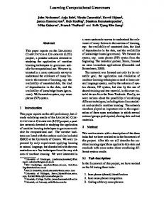
Because limm!1 �� (m) = 0, one of the two conditionals stands if m and m0 are large enough. Therefore, function different (Fig. 4) checks p = p0 with con dence level (1 ? �)2 for large enough m and m0 . In our algorithm � will slowly change with the size of the sample (at most linearly), but even in this case �� has the correct limit. Indeed, its logarithmic dependence on � makes the result depend moderately on this value. 9
algorithm different 0 0 input: output: begin algorithm 0 0 if return true else return false endif end algorithm
f; m; f ; m ; � boolean
jf=m ? f =m j < ��(m) + ��(m0 ) then
Figure 4: Algorithm different.
References
� Aho, A.V. and Ullman, J.D. (1972): \The theory of parsing, translation
� � � � � � � � �
and compiling. Volume I: Parsing". Prentice-Hall, Englewood Cli�s, NJ. Angluin, D. (1982): Inference of reversible languages. Journal of the Association for Computing Machines 29, 741{765. Angluin, D. (1988): Identifying languages from stochastic examples. Yale University Technical Report: YALEU/DCS/RR{614. Carrasco, R.C. and Oncina, J. (1994): Learning stochastic regular grammars by means of a state merging method in \Grammatical Inference and Applications" (R.C. Carrasco and J. Oncina, Eds.). Lecture Notes in Arti cial Intelligence 862, Springer-Verlag, Berlin. Gold, E.M. (1967): Language identi cation in the limit. Information and Control 10, 447{474. Hoe�ding, W. (1963): Probability inequalities for sums of bounded random variables. American Statistical Association Journal 58, 13{30. Hopcroft, J.E. and Ullman, J.D. (1979): \Introduction to automata theory, languages and computation". Addison Wesley, Reading, Massachusetts. Oncina, J. and Garc��a, P. (1994): Inference of rational tree sets. Universidad Polit�ecnica de Valencia, Internal Report DSIC-ii-1994-23. Sakakibara, Y. (1992): E�cient learning of context-free grammars from positive structural examples. Information and Computation 97, 23{60. Stolcke, A. and Omohundro, S. (1993): Hidden Markov model induction by bayesian model merging in \Advances in Neural Information Processing Systems 5" (C.L. Giles, S.J. Hanson and J.D. Cowan, Eds.). MorganKaufman, Menlo Park, California.
10