sep â separability(newSet) for jj = 1 to numT weaks do. tempSet â tweak(newSet). tempSep â separability(tempSet) if tempSep ⥠sep then sep â tempSep.
Learning Discriminative Local Patterns with Unrestricted Structure for Face Recognition Douglas Brown, Yongsheng Gao, Jun Zhou School of Engineering Griffith University Brisbane, Australia {douglas.brown, yongsheng.gao, jun.zhou}@griffith.edu.au Abstract—Local binary patterns are a popular local texture feature for describing textures and objects. The standard method and many derivatives use a hand-crafted structure of point comparisons to encode the local texture to build the descriptors. In this paper we propose automatically learning a discriminative pattern structure from an extended pool of candidate pattern elements, without restricting the possible configurations. The learnt pattern structure may contain elements describing many different scales and gradient orientations that are not available in LBP (and related patterns), thus allowing the flexibility to construct structures capable of better representing the objects under test. We show through experimentation on two face recognition databases that this approach consistently outperforms other methods, in terms of training speed and recognition accuracy in every tested case.
I.
I NTRODUCTION
Face recognition using local features is an active research area [1]–[5]. These approaches are robust to various changes in facial expression, pose, slight misalignment [2], illumination and certain occlusions when compared with holistic methods [6], [7]. Among these local features, one prevalent local texture feature is the Local Binary Pattern [8]. It is computationally simple and performs well in terms of accuracy. It has been shown to perform especially well when used for face recognition [9]. LBP and its derivatives have been shown to be effective when applied to applications such as texture representation [2], gender determination [10], face and object detection and recognition [11], facial expression analysis, image and video retrieval and other applications [12]. Its effectiveness is evident in the numerous applications and variations on the original method presented in literature; examples of approaches based on LBP include incorporating and combining LBP of colours [13]; extending the neighbourhood size of the extracted pattern [8]; completing LBP [14], where the ring and centre pixels are compared to both the image average intensity as well as the centre pixel; the list goes on. In fact, there are over 100 methods based on LBP, as reviewed in [12]. The original LBP method extracts an eight bit code for each small neighbourhood of pixels surrounding each pixel. A histogram of code frequencies is then built from the codes within a defined region to form the texture feature for that region. For face recognition, the texture features generally consist of concatenated histograms of LBP micropattern texture codes extracted from each region of the subdivided face image [9]. The image may be transformed prior to LBP extraction, using Gabor transforms, directional derivatives [2], learned
filters [3] or another transform, to improve the performance of the features. Alternately (or additionally) the histogram of micropattern codes may be transformed after extraction to reduce the length of the features and to improve classification speed and accuracy, by merging bins [2], using uniform patterns [11], selecting dominant [15] or discriminative [16] bins, learning through boosting [17], or other code selection methods. The original method involves extracting consecutive points on a ring and comparing each with a reference, which is always the intensity of the centre pixel, and then encoding the sign of the comparison result. The majority of derivative methods utilise this structure. In other cases the ring is replaced with another hardcoded geometry. For example, elongated LBP [18] distorts the standard ring configuration into an ellipse having a defined angle to encode more anisotropic characteristics and modify the response to better capture different gradient directions present in the image. Another example is shrink-boost histogram learning [17], which provides a fixed extended pool of micropatterns then iteratively alternates between boosting and discarding less-discriminative bins from the histogram. The pattern pool is fixed and only defined for a 3x3 neighbourhood. The fundamental LBP utilises a 3x3 pixel neighbourhood, but has been extended to multiple neighbourhood and ring sizes to better performance at different scales [8]. The LBP micropattern pixel pair comparison setup for a 5x5 pixel neighbourhood is similar to that shown in Fig. 2. The comparison of the eight fixed pixel neighbours of the centre pixel gives greyscale derivatives in eight directions, with pixels compared having roughly constant distance, using bilinear interpolation of the pixel intensity for larger neighbourhood sizes. We believe that this arbitrarily chosen fixed geometry and forced comparison with the centre pixel limits the discrimination effectiveness of the LBP. In [5], Maturana et al. proposed a Discriminative Local Binary Pattern (DLBP), which compares the centre pixel with any other pixel in the neighbourhood, rather than limiting the comparison to just the points on the ring. They learn an effective set of b relationships to be used to form the b-bit binary code using a stochastic hill climbing routine maximizing a Fisher-like separation criteria of the histograms, shown (1), over the images in the training set.
Sep =
(μw − μb )2 2 + σ2 σw b
(1)
In this equation, μw and μb represent the average distance between histograms within the same class and between different classes, respectively, and σw and σb are the standard deviations of the distances. This approach shows better performance than standard LBP and some other derivatives, because it can learn an improved pattern structure based on a set of pixel relationships rather than relying on an arbitrary ring organization. However, DLBP, like most of the hand-crafted patterns, relies on comparison of neighbouring pixels with the arbitrarily chosen centre pixel, which means that the maximum distance between any two pixels to be compared is half of the neighbourhood dimensions, thus limiting the effective frequency range, or scale, that can be coded for a given pixel range. It also limits the number of possible angles of the relationships, which limits the number of possible discrete gradient directions that relationships may describe effectively. Finally, the use of the centre pixel in each comparison limits the amount of pixel information that may be encoded for a given pixel neighbourhood, meaning that a complete set of eight comparisons only contains information from nine points from within the neighbourhood. We believe that parts of an image may be more effectively coded using additional relationships not possible with DLBP. In our method we do not have any fixed arbitrary relationships; we believe that the descriptor effectiveness can be improved by providing a larger pool of pattern geometries to choose from. We call this new approach Unrestricted Structure Learned Discriminative Local Pattern (US-LDLP). We would like to point out that although US-LDLP is applied to face recognition in this paper, this approach is quite general and can be extended to other computer vision applications. In the next sections we will describe our method, the learning of the micropattern structure, recognition approach, separation scores and results of testing the feature on two face databases and finally the discussion and conclusion.
Fig. 2. The standard organisation of pixel comparisons in LBP. The pattern is encoded in a clockwise direction using (2) to obtain 100000112 (13110 ) for the neighbourhood shown.
Fig. 3. Geometry of an example set of pixel comparisons in DLBP. The pattern is encoded according to the order in which the learning routine defines them, using (2). The neighbourhood depicted will be encoded as 100000112 (13110 ).
Fig. 1. An example 5x5 neighbourhood of pixel intensities used by the methods in Fig. 2, 3 and 4 . The numbers represent pixel intensity values and depict a region with a dominant gradient direction from top left to bottom right.
Fig. 4. Geometry of an example set of pixel comparisons in US-LDLP. The pattern is encoded according to the order in which the learning routine defines them, using (4). The neighbourhood depicted will be encoded as 111111112 (25510 ).
II.
U NRESTRICTED S TRUCTURE L EARNED D ISCRIMINATIVE L OCAL PATTERNS
US-LDLP has an increased number of usable pixel relationships, increased range of scales and an increased precision of directions over DLBP and LBP of the same neighbourhood size. As an example, US-LDLP operating on a 3x3 neigh�9 � bourhood has a pool of = 36 available pixel relationships 2 √ and 2 2 pixels distance between compared points, whereas DLBP would be operating in a degenerate mode equivalent to standard LBP, with only eight possible comparison elements to learn from and half the scale of US-LDLP. For a 5x5 neighbourhood, DLBP has 5√2 − 1 = 24 available relationships, with � a�maximum scale of 2 2, whereas US-LDLP has√a pool of 25 2 = 300 relationships with maximum scales of 4 2 and many more directions. For LBP and DLBP, the micropattern code is formed for each neighbourhood using equation (2), where u(·) is the unit step function, shown in equation (3), ai is the pixel intensity of a radial satellite point and b is the centre reference point. c=
8 �
u(ai − b) · 2i−1
(2)
i=1
� u(x) =
1, if x ≥ 0 0, otherwise
(3)
This builds up an eight bit string of the binary outputs of the comparisons, formed into an integer value. For LBP, the satellite points, ai , are located at equally spaced points around a circle centred on point b and the comparisons are made in a clockwise direction. This allows phenomena such as uniform patterns, termed LBPu2 in [8], to be observed. This kind of ordering is not meaningful to DLBP and US-LDLP. For US-LDLP, as there is no common fixed element b, the micropattern code is formed using equation (4), where ai and bi are the intensity of the first and second pixels, respectively, in each element in the set of pixel pair relationships.
c=
8 �
u(ai − bi ) · 2i−1
(4)
i=1
Fig. 4 shows the structure of an example US-LDLP pattern on a pixel neighbourhood; it is clear that the pattern is not restricted like those in Fig. 2 and Fig. 3. In practice, any pair of pixels within the neighbourhood can constitute an structure element of the US-LDLP micropattern. The greater variation in utilised orientations and scales is evident. Due to the manner in which the micropatterns are coded, it is easy to see that these approaches may be applied to greyscale images, or to images in various transformation spaces (Tan & Triggs, Gabor, directional derivatives and so on), just as is possible with LBP and some derivative works [2], [4]. In the rest of this paper, all examples and experiments will use the eight bit codes for all methods; these are the most common in the literature and provide a good trade-off between performance and speed, in addition to allowing the performances of the different methods to be directly compared.
Algorithm 1 Stochastic Hill Climbing Structure Learning procedure LEARN SHC set ← [initial guess] bestSep ← −∞ for hh = 1 to numIterations do newSet ← set sep ← separability(newSet) for jj = 1 to numT weaks do tempSet ← tweak(newSet) tempSep ← separability(tempSet) if tempSep ≥ sep then sep ← tempSep newSet ← tempSet end if end for set ← newSet if sep ≥ sepBest then bestSet ← set bestSep ← sep end if end for return bestSep, bestSet end procedure procedure TWEAK(set) set[rand] ← select rand in (f ullP ool \ set) return set end procedure procedure SEPARABILITY(set) hist[...] ← get histograms(images[...], set) calculate distance between every pair of histograms calculate intra- and extra-class μ and σ from distances 2 return (μw − μb )2 /(σw + σb2 ) end procedure
III.
L EARNING PATTERN S TRUCTURES
Each micropattern can be seen as a bitwise concatenation of the results of a number of pixel intensity comparisons. As a means of selecting the best pixel relationships to use in creating the final pattern structure, a learning algorithm can be employed, such as modified boosting, incremental classifier building, selecting the most discriminative comparison element from a random pool of possible pixel pair relationships or stochastic hill climbing. Incremental classifier building can be accomplished by building up the structure one pixel pair comparison at a time, choosing the pair such that the separability score of the resulting set is maximized. Stochastic hill climbing (SHC) may be implemented using multiple rounds of random ”tweaks” applied to the set of pixel pair relationships, i.e. replacing a random element from the set with one randomly chosen from the pool, and retaining the tweaked set having improved performance from each round for use in the next round [5].
Options such as boosting or other classifier learning techniques may be applied to all possible pixel pair comparison outputs for each image section to be trained. During training, the weakest-weighted elements can be excluded from the final pattern structure. Out of the methods trialled, SHC was found to be the most effective learning instrument for a large number of pixel pair relationships. The SHC algorithm detailed in the listing shown in Algorithm 1 is based on [5]. The SHC algorithm uses 60 iterations, or rounds, and 30 structure element tweaks within each round, as proposed in [5]. During each round, if a tweak improves the separation score of the pattern structure, the tweaked structure is used as the basis for the next tweak. Conversely, if the tweak results in a worse-performing structure, the tweak will be reverted so that the separation score of the structure being learnt can never decrease during training. The SHC approach is notably more effective than comparing separation scores of the equivalent number of randomly selected sets. Even though the pool of structure element candidates for US-LDLP is much larger than for DLBP, the learning time complexity and memory consumption is the same for USLDLP as for DLBP and the matching complexity for USLDLP, DLBP and LBP are identical. The SHC method is effective at improving the separability score of a classifier set. It can easily be run in parallel across multiple processors, however the large size of the features and the number of iterations makes it a computationally intensive method. The learning time complexity and memory usage increases approximately in proportion to the product of the number of partitions and the number of bins in the histograms. To improve on these costs, the number of histogram bins can be reduced prior to calculating the separability score, e.g. by merging neighbouring bins [2], discarding universally empty bins, using only dominant patterns [15] or using the most descriptive bins [16]. All of these methods are efficient for reducing the feature dimensionality during training, allowing for reductions in training time and memory resource requirements. On an i7 3.5GHz machine, training a single partition in MATLAB requires a time period approaching 30 seconds. The distance metric used in training and testing is the histogram intersection distance, due to its simplicity, speed and acceptable performance. The histogram intersection equation is shown in (5). �2b min(Ai , Bi ) dHI (A, B) = 1 − i=1�2b (5) i=1 Bi Other distance metrics are also valid; examples include the �1 norm or Manhattan distance used in [5] and the χ2 distance employed in [11]. A number of methods use different weighting for each partition to improve the overall match accuracy; in this paper we treat each partition equally, which still allows for a valid comparison of the performance of the different local pattern representations. IV.
E XPERIMENT
A. Databases The LBP, LBP-U2, DLBP and US-LDLP can be used to extract features from any image for a variety of applications. In this paper, we apply the methods to face recognition, and
test against images from the cropped greyscale AR [19] and FERET [20], [21] databases. The AR database subset consists of cropped and aligned images for 100 persons, consisting of 26 images for each person, taken under a variety of pose, expression, occlusion and lighting conditions in two sessions, spaced two weeks apart, for a total of 2600 images. These images have been cropped to 165 x 120 pixels. We use the first three unoccluded images for training the pattern structures and as the gallery. The remaining 23 images per person are used as the probe images and include occlusion and various illumination effects. Sample cropped images from the AR database are shown in the top row of Fig. 5; the occlusion caused by sunglasses and scarf, as well as the difference in lighting source can be seen.
Fig. 5. Example images from the datasets. The face images in the top row are samples from the AR dataset, those in the second row are from the FERET dataset, and the final row is composed of the Tan & Triggs [4] normalised versions of the images in the second row.
The FERET database subset includes cropped frontal images where five or more images of each person are available, for a total of 905 images depicting 117 persons. These images have been cropped to 160 x 160 pixels. The first three images from each person’s subset contribute to the training set and gallery; the remainder are used as the probe images. Sample cropped images from the FERET database are shown in the second row of Fig. 5. There are a number of variations in lighting and expressions, with some changes in pose in the probe and gallery images. Learning is performed on the same image subset that forms the gallery. For both datasets, only the first 3 images for each person are used, which represent some relatively neutral expressions without occlusions. The use of only a small subset of the faces reduces the training time and shows that the experiments are more easily applied to real applications where potentially few gallery images are available. The experiment is conducted for cropped database images in addition to the same images after applying Tan & Triggs normalisation [4]. The normalisation is designed to provide invariance to changes in lighting sources. Because both datasets contain images with varying illumination, it is logical that the performance will increase for the normalised images. The normalisation process is rather quick, and not all stages described in [4] need to be carried out, namely the final contrast equalisation step is not required due to the monotonic greyscale invariance exhibited by the micropattern codes defined in (2) and (4). The Tan & Triggs normalised images give better performance for all methods. In the following sections, only
DĂƚĐŚ��ĐĐƵƌĂĐLJ�;йͿ
ϵϱ
�Z�ϱdžϱ
ϵϬ
�>�W h^Ͳ>�>W >�W >�WƵϮ
ϴϬ ϳϱ
DĂƚĐŚ��ĐĐƵƌĂĐLJ�;йͿ
ϵϳ
�>�W h^Ͳ>�>W >�W >�WƵϮ
ϵϲ ϵϱ ϵϰ
ϯdžϰ
ϱdžϲ
ϳdžϳ ϴdžϴ ϭϬdžϭϬ WĂƌƚŝƚŝŽŶ��ƌƌĂŶŐĞŵĞŶƚ
ϭϮdžϭϮ
ϭϲdžϭϮ
Fig. 8. Match results for the FERET dataset (Tan & Triggs normalised) using a 5x5 neighbourhood ϯdžϰ
ϱdžϲ
ϳdžϳ ϴdžϴ ϭϬdžϭϬ WĂƌƚŝƚŝŽŶ��ƌƌĂŶŐĞŵĞŶƚ
ϭϮdžϭϮ
ϭϲdžϭϮ
ϭϬϬ ϵϵ
Fig. 6. Match results for the AR dataset (Tan & Triggs normalised) using a 5x5 neighbourhood
ϵϱ
ϵϴ
ϵϮ
ϳϬ
ϭϬϬ
&�Z�d�ϱdžϱ
ϵϯ
ϴϱ
ϲϱ
ϵϵ
�Z�ϳdžϳ
DĂƚĐŚ��ĐĐƵƌĂĐLJ�;йͿ
ϭϬϬ
ϭϬϬ
DĂƚĐŚ��ĐĐƵƌĂĐLJ�;йͿ
the results for the experiment carried out on the normalised images is shown; the trends (i.e. the relative performance of the different methods) described in the results are evident for images with and without normalisation.
&�Z�d�ϳdžϳ
ϵϴ ϵϳ
�>�W h^Ͳ>�>W >�W >�WƵϮ
ϵϲ ϵϱ ϵϰ ϵϯ
ϵϬ
ϵϮ
�>�W h^Ͳ>�>W >�W >�WƵϮ
ϴϱ ϴϬ
ϯdžϰ
ϱdžϲ
ϳdžϳ ϴdžϴ ϭϬdžϭϬ WĂƌƚŝƚŝŽŶ��ƌƌĂŶŐĞŵĞŶƚ
ϭϮdžϭϮ
ϭϲdžϭϮ
Fig. 9. Match results for the FERET dataset (Tan & Triggs normalised) using a 7x7 neighbourhood FIX THE LEGEND e.g. US-LDLP-7
ϳϱ ϳϬ ϯdžϰ
ϱdžϲ
ϳdžϳ ϴdžϴ ϭϬdžϭϬ WĂƌƚŝƚŝŽŶ��ƌƌĂŶŐĞŵĞŶƚ
ϭϮdžϭϮ
ϭϲdžϭϮ
Fig. 7. Match results for the AR dataset (Tan & Triggs normalised) using a 7x7 neighbourhood FIX THE LEGEND e.g. US-LDLP-7
the 3x4 partition size and 7x7 neighbourhood size, the LBP, LBPu2 , DLBP and US-LDLP attain accuracies, respectively, of 96.39%, 92.96%, 95.85% and 97.65%. C. Separation Performance
B. Face Recognition Performance The task of face recognition is performed using a forcedmatch nearest neighbour approach, using the histogram intersection distance as the dissimilarity score. The features are kept as full concatenated histograms to provide an indicative baseline performance, although using bin selection methods described in previous sections can be employed to gain improvements in efficiency and accuracy. Fig. 6 and Fig. 7 shows the accuracy of the LBP, LBPu2 , DLBP and US-LDLP methods when applied to the AR database, for neighbourhood sizes of 5x5 and 7x7 pixels, respectively. The US-LDLP method can clearly be seen to outperform or match all other methods for every partition configuration and for every neighbourhood size. For the 3x4 partition size, where the accuracies haven’t yet saturated, with a 7x7 neighbourhood size, the LBP, LBPu2 , DLBP and US-LDLP attain accuracies of 79.04%, 71.61%, 80.04% and 85.26%, respectively. Fig. 8 and Fig. 9 show the accuracy of the methods when matching images in the FERET database. Again, the USLDLP method can be seen to dominate the other methods across all partition arrangements and neighbourhood sizes. For
The separation scores (see equation (1)) for LBP, LBPu2 , DLBP and US-LDLP are shown in Fig. 10 and Fig. 11 when trained on the AR and FERET datasets, respectively. The figures show results for the 7x7 neighbourhood, however the smaller 5x5 neighbourhood had the same trends, while the 3x3 neighbourhood is unsuitable for training DLBP. From the figures, US-LDLP can be seen to have superior separation compared to DLBP. The average separation scores for LBP and LBPu2 , which are not the result of training, are reported below the figures. During the learning phase, the rate at which DLBP and US-LDLP converge to their final pattern structure can be seen in Fig. 10 and Fig. 11. Each line in this figure represents the mean separation score of the micropattern structure from a 7x7 pixel neighbourhood at each round of training. These measures were calculated over all partitions from all partitioning layouts, for a total of 1182 partitions, to provide a large sample size to improve the confidence interval and smooth the reported values. The partition schemes result in the image being subdivided into 3x4, 5x6, 7x7, 8x8, 10x10, 12x12 and 16x12 blocks. The separation scores of the LBP and LBPu2 are 1.00 and 0.91, respectively, on the AR dataset, and 0.75 and 0.59, respectively, on the FERET dataset. With even a single round
of training, the average US-LDLP separation scores are well above the LBP and LBPu2 values. From the above results, it is clear that learning the micropattern structure allows for more-discriminative features. The figures show the separation superiority of the USϭ͘ϳ
�Z�ϳdžϳ
^ĞƉĂƌĂƚŝŽŶ�^ĐŽƌĞ
ϭ͘ϲ ϭ͘ϱ
h^Ͳ>�>W �>�W
ϭ͘ϰ ϭ͘ϯ ϭ͘Ϯ ϭ͘ϭ ϭ Ϭ
ϭϬ
ϮϬ
ϯϬ dƌĂŝŶŝŶŐ�ZŽƵŶĚ
ϰϬ
ϱϬ
ϲϬ
Fig. 10. Separation score during training for the AR dataset (Tan & Triggs normalised) using a 7x7 neighbourhood. The comparative LBP separation score is 1.00, while the LBPu2 separation score is 0.91.
ϭ͘ϭ ϭ͘Ϭϱ
&�Z�d�ϳdžϳ
^ĞƉĂƌĂƚŝŽŶ�^ĐŽƌĞ
ACKNOWLEDGMENT Portions of the research in this paper use the FERET database of facial images collected under the FERET program, sponsored by the DOD Counterdrug Technology Development Program Office. R EFERENCES
ϭ
h^Ͳ>�>W �>�W
Ϭ͘ϵϱ Ϭ͘ϵ Ϭ͘ϴϱ Ϭ͘ϴ Ϭ͘ϳϱ
techniques, but makes use of micropattern structures that are based on a hand-crafted arrangement of pixel relationships, which reduces its potential effectiveness. In this paper we have shown through extensive testing on images from the AR and FERET datasets that there are more effective patterns that may be learned based on the training data. We have also shown the proposed US-LDLP approach can learn discriminative relationships much faster than the more restricted DLBP. In fact, the averaged Fisher separation score of US-LDLP was seen to exceed that of DLBP after less than one twentieth of the number of training rounds. The matching results also show that US-LBP has superior performance compared with the other tested methods, across all trialled experimental configurations. In this paper we have shown that selecting the pixel relationships for local texture patterns using learning, without restricting the pool of possible relationships, provides superior recognition accuracy and faster training times.
Ϭ
ϭϬ
ϮϬ
ϯϬ dƌĂŝŶŝŶŐ�ZŽƵŶĚ
ϰϬ
ϱϬ
ϲϬ
Fig. 11. Separation score during training for the FERET dataset (Tan & Triggs normalised) using a 7x7 neighbourhood. The comparative LBP separation score is 0.75, while the LBPu2 separation score is 0.59.
LDLP over the more restricted DLBP selection method. It appears that the DLBP separation score saturates before the end of training, whereas the score for US-LDLP can be seen to continue to be increasing even at the last iteration. Further improvements in separation could be gained by increasing the number of training rounds. The averaged separation score of US-LDLP after three training rounds can be seen to eclipse that of DLBP after even sixty rounds. Based on this observation, the training time could be reduced greatly, while still attaining a separation score exceeding that of DLBP, LBP and LBPu2 . The potential for growth and the rate of change of the score with each training round is visible for US-LDLP, whereas DLBP shows much less improvement after the initial rounds. V.
C ONCLUSION
Local features are an important tool in pattern recognition for a variety of applications. LBP is one of the most popular
[1] B. Gkberk, M. O. irfanoglu, L. Akarun, and E. Alpaydn, “Learning the best subset of local features for face recognition,” Pattern Recognition, Vol, vol. 40, pp. 1520–1532, 2007. [2] B. Zhang, Y. Gao, S. Zhao, and J. Liu, “Local derivative pattern versus local binary pattern: Face recognition with high-order local pattern descriptor,” IEEE Trans. Image Process., vol. 19, no. 2, pp. 533–544, 2010. [3] Z. Lei, D. Yi, and S. Li, “Discriminant image filter learning for face recognition with local binary pattern like representation,” in IEEE Conf. Comput. Vis. and Pattern Recognit., 2012, pp. 2512–2517. [4] X. Tan and B. Triggs, “Enhanced local texture feature sets for face recognition under difficult lighting conditions,” IEEE Trans. Image Process., vol. 19, no. 6, pp. 1635–1650, 2010. [5] D. Maturana, D. Mery, and A. Soto, “Learning discriminative local binary patterns for face recognition,” in IEEE International Conf. Autom. Face & Gesture Recognit. and Workshops. IEEE, 2011, pp. 470–475. [6] M. Turk and A. Pentland, “Face recognition using eigenfaces,” in Computer Vision and Pattern Recognition, 1991. Proceedings CVPR ’91., IEEE Computer Society Conference on, 1991, pp. 586–591. [7] P. Belhumeur, J. Hespanha, and D. Kriegman, “Eigenfaces vs. fisherfaces: recognition using class specific linear projection,” Pattern Analysis and Machine Intelligence, IEEE Transactions on, vol. 19, no. 7, pp. 711–720, 1997. [8] T. Ojala, M. Pietikainen, and T. Maenpaa, “Multiresolution gray-scale and rotation invariant texture classification with local binary patterns,” Pattern Analysis and Machine Intelligence, IEEE Transactions on, vol. 24, no. 7, pp. 971–987, 2002. [9] T. Ahonen, A. Hadid, and M. Pietik¨ainen, “Face recognition with local binary patterns,” in European Conf. Comput. Vis. Springer, 2004, pp. 469–481. [10] A. Shobeirinejad and Y. Gao, “Gender classification using interlaced derivative patterns,” in International Conf. Pattern Recognit. IEEE, 2010, pp. 1509–1512. [11] T. Ahonen, A. Hadid, and M. Pietikainen, “Face description with local binary patterns: Application to face recognition,” IEEE Trans. Pattern Anal. and Mach. Intell., vol. 28, no. 12, pp. 2037–2041, 2006.
[12] D. Huang, C. Shan, M. Ardabilian, Y. Wang, and L. Chen, “Local binary patterns and its application to facial image analysis: A survey,” IEEE Trans. Syst., Man, and Cybern., Part C: Appl. and Rev., vol. 41, no. 6, pp. 765–781, 2011. [13] J.-Y. Choi, Y.-M. Ro, and K. Plataniotis, “Color local texture features for color face recognition,” Image Processing, IEEE Transactions on, vol. 21, no. 3, pp. 1366–1380, 2012. [14] Z. Guo, L. Zhang, and D. Zhang, “A completed modeling of local binary pattern operator for texture classification,” IEEE Trans. Image Process., vol. 19, no. 6, pp. 1657–1663, 2010. [15] S. Liao, M. Law, and A. Chung, “Dominant local binary patterns for texture classification,” IEEE Trans. Image Process., vol. 18, no. 5, pp. 1107–1118, 2009. [16] Y. Guo, G. Zhao, M. Pietik¨ainen, and Z. Xu, “Descriptor learning based on fisher separation criterion for texture classification,” in Asian Conf. Comput. Vis. Springer, 2011, pp. 185–198. [17] C.-K. Heng, S. Yokomitsu, Y. Matsumoto, and H. Tamura, “Shrink boost for selecting multi-lbp histogram features in object detection,” in IEEE Conf. Comput. Vis. and Pattern Recognit., 2012, pp. 3250–3257. [18] S. Liao and A. C. Chung, “Face recognition by using elongated local binary patterns with average maximum distance gradient magnitude,” in Computer Vision–ACCV 2007. Springer, 2007, pp. 672–679. [19] A. M. Martinez and R. Benavente, “The ar face database,” CVC Tech. Report #24, 1998. [20] P. J. Phillips, H. Wechsler, J. Huang, and P. Rauss, “The feret database and evaluation procedure for face recognition algorithms,” Image and Vision Comput. J., vol. 16, no. 5, pp. 295–306, 1998. [21] P. J. Phillips, H. Moon, S. A. Rizvi, and P. Rauss, “The feret evaluation methodology for face recognition algorithms,” IEEE Trans. Pattern Anal. and Mach. Intell., vol. 22, pp. 1090–1104, 2000.