Learning Efficient Reactive Behavioral Sequences from Basic Reflexes in a Goal-Directed Autonomous Robot ´ Jos´ e del R. MILLAN Institute for Systems Engineering and Informatics Commission of the European Communities. Joint Research Centre TP 361. 21020 ISPRA (VA). ITALY e-mail:
[email protected]
Abstract
proach to control of autonomous mobile robots is that of reactive systems (e.g., Brooks, 1986; Connell, 1990; Schoppers, 1987). However, there exist two reasons to prefer a robot that acquires automatically the appropriate navigation strategies. First, a learning approach can considerably reduce the robot programming cost. Second and most importantly, pure reactive controllers may generate inneficient trajectories since they select the next action as a function of the current sensor readings and the robot’s perception is limited. Autonomous robots can adapt to unknown environments in two ways. The first one is to acquire a coarse global map of them. This map is made out of landmarks and is built from sensory data. Then, planning takes place at an abstract level and all the low level details are handled by the reactive component as the robot actually moves (e.g., Connell, 1992; Mataric, 1992; Miller & Slack, 1991). The second adaptive approach is to learn directly the appropriate reactive behavioral sequences (e.g., Lin, 1991; Mill´an, 1992; Mill´an & Torras, 1992; Mitchell & Thrun, 1993). While we agree that global maps are very helpful for navigation, we believe that the addition of learning capabilities to reactive systems are sufficient to allow a robot to generate efficient trajectories after a limited experience. This paper presents experimental results that support this claim: a real autonomous mobile robot equipped with low-resolution sensors learns efficient goaloriented obstacle-avoidance reactive sequences in a few trials. This paper describes TESEO, an autonomous mobile robot controlled by a neural network. The neural controller maps the current perceived situation into the next action. A situation is made of sensory information coming from physical as well as virtual sensors. This neural network offers two advantages, namely good generalization capabilities and high tolerance to noisy sensory data. TESEO improves its performance through reinforcement learning (Barto et al., 1983; Barto et al.,
This paper describes a reinforcement connectionist learning mechanism that allows a goaldirected autonomous mobile robot to adapt to an unknown indoor environment in a few trials. As a result, the robot learns efficient reactive behavioral sequences. In addition to quick convergence, the learning mechanism satisfies two further requirements. First, the robot improves its performance incrementally and permanently. Second, the robot is operational from the very beginning, what reduces the risk of catastrophic failures (collisions). The learning mechanism is based on three main ideas. The first idea applies when the neural network does not react properly to the current situation: a fixed set of basic reflexes suggests where to search for a suitable action. The second is to use a resource-allocating procedure to build automatically a modular network with a suitable structure and size. Each module codifies a similar set of reaction rules. The third idea consists on concentrating the exploration of the action space around the best actions currently known. The paper also reports experimental results obtained with a real mobile robot that demonstrate the feasibility of our approach.
1 Introduction In this paper, we investigate how a goal-directed autonomous mobile robot can rapidly adapt its behavior in order to navigate efficiently in an unknown indoor environment. Efficient navigation strategies are common in animals (see Gallistel (1990) for a review) and are also critical for autonomous robots operating in hostile environments. In the case of unknown environments, a common apThis paper will appear in From Animals to Animats: Third International Conference on Simulation of Adaptive Behavior, Brighton, UK, August 8-12, 1994.
1
1989; Sutton, 1984; Watkins, 1989; Williams, 1992) and adapts itself permanently as it interacts with the environment. An important assumption of our approach is that the robot receives a reinforcement signal after performing every action. Thus TESEO’s aim is to learn to perform those actions that optimizes the total reinforcement obtained along the trajectory to the goal. Although this assumption is hard to satisfy in many reinforcement learning tasks, it is not in the case of goal-directed tasks since the robot can easily evaluate its progress towards the goal at any moment. A second assumption of our approach is that the goal location is known. In particular, the goal location is specified in relative cartesian coordinates with respect to the starting location. TESEO overcomes three common limitations associated to basic reinforcement connectionist learning. The first and most important one is that reinforcement learning might require an extremely long time. The main reason is that it is hard to determine rapidly promising parts of the action space where to search for suitable reactions. The second limitation is related to the first one and concerns the inability of “monolithic” connectionist networks —i.e., networks where the knowledge is distributively codified over all the weights— to support incremental learning. In this kind of standard networks, learning a new rule (or tuning an existing one) could degrade the knowledge already acquired for other situations. Finally, the third limitation regards the robot’s behavior during learning. Practical learning robots should be operational at any moment and, most critically, they should avoid catastrophic failures such as collisions.
Sonar Sensors
Infrared Sensors
Tactile Sensors
Figure 1. The Nomad 200 mobile robot.
the interval [0, 1]. The first 32 components correspond to the infrared and sonar sensor readings. In this case, a value close to zero means that the corresponding sensor is detecting a very near obstacle. The remaining 8 components are derived from a virtual sensor that provides the distance between the current and goal robot locations. This sensor is based on the dead-reckoning system. These 8 components correspond to a coarse codification of an inverse exponential function of the virtual sensor reading. The main reason for using this codification scheme is that, since it achieves a sort of interpolation, it offers three theoretical advantages, namely a greater robustness, a greater generalization ability and faster learning. The output of the connectionist network consists of a single component that controls directly the steering motor and indirectly the translation and rotation motors. This component is a real number in the interval [−180, 180] and determines the direction of travel with respect to the vector connecting the current and goal robot locations. Once the robot has steered the commanded degrees, it translates a fixed distance (10 inches) and, at the same time, it rotates its turret in order to maintain the front infrared and sonar sensors oriented toward the goal. It is worth noting that a relative codification of both the physical sensor readings and the motor command enhances TESEO’s generalization capabilities.
2 Experimental Setup The physical robot is a wheeled cylindrical mobile platform of the Nomad 200 family (see Figure 1). It has three independent motors. The first motor moves the three wheels of the robot together. The second one steers the wheels together. The third motor rotates the turret of the robot. The robot has 16 infrared sensors and 16 sonar sensors that provide distances to the nearest obstacles the robot can perceive, and 20 tactile sensors that detect collisions. The infrared and sonar sensors are evenly placed around the perimeter of the turret. Finally, the robot has a dead-reckoning system that keeps track of the robot’s position and orientation. As stated before, the connectionist controller uses the current perceived situation to compute a spatially continuous action. Then, the controller waits until the robot has finished to perform the corresponding motor command before computing the associated reinforcement signal and the next action. We will describe next what the input, output and reinforcement signals are. The input to the connectionist network consists of a vector of 40 components, all of them real numbers in 2
Evaluator
The reinforcement signal is a real number in the interval [−3, 0] which measures the cost of doing a particular action in a given situation. The cost of an action is directly derived from the task definition, which is to reach the goal along trajectories that are sufficiently short and, at the same time, have a wide clearance to the obstacles. Thus actions incur a cost which depends on both the step clearance and the step length. Concerning the step clearance, the robot is constantly updating its sensor readings while moving. Thus the step clearance is the shortest distance provided by any of the sensors while performing the action. Finally, TESEO has a low-level asynchronous emergency routine to prevent collisions. The robot stops and retracts whenever it detects an obstacle in front of it which is closer than a safety distance.
z
e1 1
x1
bj
e 1i
¼
x2
b1
ej
1
e nj
3 The Reinforcement Approach Situation
TESEO’s learning task is to associate with every per-
ceived situation the action that optimizes the total reinforcement in the long-term (i.e., from the moment this action is taken until the goal is reached). To solve it, TESEO uses two different learning rules, namely temporal difference (TD) methods (Sutton, 1988) and associative search (AS) (Barto et al., 1983; Sutton, 1984; Williams, 1992). TD methods allow TESEO to predict the total future reinforcement it will obtain if it performs the best currently known actions that take it from its current location to the goal. AS uses the estimation given by TD to update the situation-action mapping, which is codified into the neural network. In Section 1 we mentioned that TESEO seeks to satisfy three learning requirements, namely quick convergence, incremental improvement of performance, and collision avoidance. TESEO uses three main ideas to cope with these requirements. First, instead of learning from scratch, TESEO utilizes a fixed set of basic reflexes every time its neural network fails to generalize correctly its previous experience to the current situation. The neural network associates the selected reflex with the perceived situation in one step. This new reaction rule will be tuned subsequently through reinforcement learning. Basic reflexes correspond to previous elemental knowledge about the task and are codified as simple reactive behaviors (Brooks, 1986). As the actions computed by the neural controller, the reflexes determine the next direction of travel which is followed a fixed distance while the robot rotates its turret. Each reflex selects one of the 16 directions corresponding to the current orientations of the infrared and sonar sensors. We have chosen this fixed set of directions because they are the most informative for the robot in terms of obstacle detection. It is worth noting that, except in simple cases, these reflexes alone do not generate efficient trajectories; they just provide acceptable starting points for the reinforcement learn-
M od
ul e
j
x40
Exemplar Units
Action Unit
Figure 2. Network architecture.
ing algorithm to search appropriate actions. Integrating learning and reaction in this way allows TESEO to focus on promising parts of the action space immediately and to be operational from the very beginning. Second, TESEO utilizes a resource-allocating procedure to build automatically a modular network with a suitable structure and size. Each module codifies a consistent set of reaction rules. That is, each module’s rules map similar sensory inputs into similar actions and, in addition, they have similar long-term consequences. This procedure guarantees that improvements on a module will not negatively alter other unrelated modules. Finally, TESEO explores the action space by concentrating the search around the best actions currently known. The width of the search is determined by a counter-based scheme associated to the modules. This exploration technique allows TESEO to avoid experiencing irrelevant actions and to minimize the risk of collisions.
4 Network Architecture The controller is a modular two-layer network (see Figure 2). The first layer consists of units with localized receptive fields. This means that each of these so-called exemplars represents a point of the input space and covers a limited area around this point. The activation level of an exemplar is 0 if the perceived situation is outside its receptive field and it is 1 if the situation corresponds to the point where the exemplar is centered. The second layer is made of one single stochastic linear unit. There 3
at io n
exists a full connectivity between the two layers of units. The jth module consists of the exemplars ej1 , . . . , ejn and their related links. Actions are computed after a competitive process among the existent modules: only the module that best classified the perceived situation propagates the activities of its exemplars to the output unit. The winning module, if any, is that having the highest active exemplar. In the case that no exemplar matches the perceived situation, then the basic reflexes are triggered and the current situation becomes a new exemplar. Section 6.2 provides more details about the resourceallocating procedure. Thus, in order to improve its reactions to a particular kind of situations, TESEO needs just to fit the size or to tune the weights of the module that covers that region of the input space. As pointed out before, the modules are not predefined, but are created dynamically as TESEO explores its environment. Every module j keeps track of four adaptive values. First, the expected total future reinforcement, bj , that the robot will receive if it uses this module for computing the next action. Second, the width of the receptive fields of all the exemplars of this module, dj . Third, a counter that records how many times this module has been used without improving the robot’s performance, cj . Fourth, the prototypical action the robot should normally take whenever the perceived situation is classified into this module, paj . There are as many prototypical actions as reflexes. Thus the first one is the direction of the front infrared and sonar sensors — i.e., a deviation of 0 degrees from the vector connecting the current and goal robot locations—, the second one is 22.5 degrees, and so on. Section 6.2 explains how paj is initially determined and evolves. Finally, after reacting, the evaluator computes the reinforcement signal, z, as specified in Section 2. Then, if the action was computed through the module j, the difference between z and bj is used for learning. Only the weights of the links associated to the winning module j are modified.
ej
1
pl or
pa j
Ex
pa
cj
e jk
s
Sm
+45 -45
s
+
e jn Module j Figure 3. The action unit.
separately. This exploration mechanism depends on cj , the counter associated to the winning module. The action unit transforms the contributions of the winning module j as follows. On the one hand, the exploration mechanism uses paj and cj to compute the prototypical action, pa, around which to select the output. On the other hand, the activation levels of ej1 , . . . , ejn as well as cj determine the deviation, s, from pa. Thus TESEO will perform an action which is located in the interval [pa − 45, pa + 45]. That is, TESEO will only explore actions between pa and its four neighboring prototypical actions (two to the left and two to the right). The exploration mechanism selects pa from the prototypical actions associated to all the modules that classify the perceived situation. That is, if the situation is located in the receptive field of one of the exemplars of the module m, then pam is a candidate. The selection is as follows. If cj is not divisible by, say, 3 then it chooses paj , the prototypical action of the winning module. Otherwise, it chooses the prototypical action associated to the module m with the best expected total future reinforcement, bm . The basic idea behind this exploration mechanism is that the winning module could well benefit from the knowledge of neighboring modules.
5 Action Unit As illustrated in Figure 3, the action unit’s output is a prototypical action pa plus a certain variation s that depends upon the location of the perceived situation in the input subspace dominated by the module that classifies the situation. Normally, the prototypical action is that of the winning module. As any other reinforcement system, TESEO needs to explore alternative actions for the same situation in order to discover the best action. However, this exploration is not conducted upon the whole action space, but it is performed around the best actions currently known. Since each action is the sum of two components, pa and s, the exploration mechanism works on each of them
Concerning the computation of s, an effective way of implementing exploration techniques in continuous domains is to use a stochastic process that selects with higher probability the best currently known value. This process controls separately the location being sought (mean) and the breadth of the search around that location (variance). The computation of s is done in three steps. The first step is to determine the value of the stochastic process’ parameters. The mean µ is a weighted 4
sum of the activation levels of the exemplars: µ=
n X
wkj ajk ,
action y(t) the next situation x(t + 1) belongs to the module i, and the reinforcement signal —or cost— is z(t + 1), then:
(1)
£ ¤ bj (t + 1) = bj (t) + η ∗ z(t + 1) + bi (t) − bj (t) .
k=1
wkj
where is the weight associated to the link between j ek and the action unit, and ajk is the activation level of ejk . The variance σ is proportional to cj . The basic idea is that the more times the module j is used without improving the performance of TESEO, the higher is σ. In the second step, the unit calculates its activation level l which is a normally distributed random variable: l = N (µ, σ).
Note that even if the robot reaches the module i at time t + 1, the value bi (t) is used to update bj . This makes sense, since the module i could be the same as the module j. η controls the intensity of the modification, and it takes greater values when TESEO behaves better than expected than in the opposite case. These two values of η are 0.75 and 0.075, respectively. The rationale for modifying less intensively bj when z(t+1)+bi (t)−bj (t) < 0 is that this error is probably due to the selection of an action different from the best currently known one for the module j. The problem is for TESEO to figure out bi (t) when the next situation x(t + 1) does not match any stored exemplar. In this case, bi is estimated on the basis of the distance from the next location to the goal and the distance from the next location to the perceived obstacles in between the robot and the goal. Finally, the value bj of every module j observed along a path taking to the goal is also updated in reverse chronological ®order. To do that, TESEO stores the pairs j(t), z(t + 1) , where j(t) indicates the winning module at time t. Then, after reaching the goal at time n + 1 and updating the last value bj(n) , the value bj(n−1) is updated, and so on until bj(1) . As Mahadevan and Connell (1992) point out, this technique only accelerates the convergence of the value bj of every module j —especially if it classifies situations far from the goal—, but does not change the steady value of bj .
(2)
In the third step, the unit computes s: s=
(
45, −45, l,
if l > 45, if l < −45, otherwise.
(3)
6 Learning There are four basic forms of learning in the proposed architecture. The first regards the topology of the network: initially, there exist neither exemplars nor, consequently, modules and the resource-allocating procedure creates them as they are needed. The second kind of learning concerns weight modification. The third type of learning is related to the update of the bj values and is based on TD methods. Finally, the fourth consists on the adaptation of the other three adaptive parameters associated to every module j, namely dj , cj and paj .
6.1 Temporal Difference Methods
6.2 When to Learn
Every value bj corresponds to an estimate of the total future reinforcement TESEO will obtain if it performs the best currently known actions that take it from its current location (whose associated observed situation is classified into the j th module) to the goal. Consequently, the value bj of the module j should be equal to the sum of the cost z of reaching the best next module i plus the value bi : bj =
max (z) + bi .
y∈Actions
(5)
Let us present now the three occasions in which learning takes place. The first of them arises during the classification phase, whereas the other two happen after reacting. 1. if the perceived situation is not classified into one of the existent modules —i.e., no exemplar matches it—, then the basic reflexes get control of the robot, and the resource-allocating procedure creates a new exemplar which is added either to one of the existing modules or to a new module. The new exemplar has the same coordinates as the perceived situation. That is, both represent the same point of the input space. The weight of the link from this exemplar to the action unit is initially set to zero and evolves through reinforcement learning. The new exemplar is added to one of the existing modules if its receptive field overlaps the receptive fields of the module’s exemplars and the selected reflex is the
(4)
During learning, however, this equality does not hold for the value bj of every module j because the optimal action is not always taken and, even if it is, the value bi of the next module i has not yet converged. A way of improving the quality of bj is to use the simplest TD method, i.e. TD(0). This procedure works as follows. If the situation perceived at time t, x(t), is classified into the module j, and after performing the 5
same as the module’s prototypical action. The first condition assures that every module will cover a closed input subspace. If any of the two conditions above is not satisfied, then the new exemplar is added to a new module. This module consists initially of the exemplar and its associated connections. Concerning the four parameters associated to this new module v, they are initially set to the following values: bv is estimated as when no module classifies the perceived situation (see Section 6.1), dv equals 0.5, cv equals 0, and pav is the selected reflex.
TESEO maintains the best situation-action rules known so far, while exploring other reaction rules. Finally, the adaptive parameters are also updated differently in case of reward than in case of penalty. In case of reward, dj is increased by 0.1, cj is initialized to 0, and if the output of the action unit, pa + s, is closer to a prototypical action other than paj , then paj becomes this new prototypical action. In case of penalty, cj is increased by 1 and dj is decreased by 0.1 if it is still greater than a threshold kd .
3. if (i) the perceived situation is classified into the module j, and (ii) z(t + 1) + bi (t) − bj (t) > kz then (i) the topology of the network is slightly altered, and (ii) dj is updated. If the total futute reinforcement computed after reacting, z + bi , is considerably worse the expected one, bj , this means that the situation was incorrectly classified and needs to be classified into a different module. In order for TESEO to classify this and other very similar situations into a different module the next time they will be perceived, the resource-allocating procedure modifies the network topology. Simultaneously, dj is decreased by 0.1 if it is still greater than a threshold kd . The resource-allocating procedure creates a new exemplar, eu , that has the same coordinates as the perceived situation, but it does not add it to any module. The next time this situation will be faced, eu will be the closest exemplar. Consequently, no module will classify the situation and the basic reflexes will get control of the robot. Then, the resource-allocating procedure will add eu either to one of the existing modules or to a new module as described in point 1 above. This means that our architecture classifies situations, in a first step, based on the similarity of their input representations. Then, it also incorporates task-specific information for classifying based on the similarity of reinforcements received. In this manner, the input space is split into consistent clusters since a similar total future reinforcement corresponds to similar suitable actions for similar situations in a given input subspace.
2. if (i) the perceived situation is classified into the module j, and (ii) z(t + 1) + bi (t) − bj (t) ≤ kz , where kz is a constant, then (i) the exemplars of that module, ej1 , . . . , ejn , are modified to make them closer to the situation, (ii) the weights associated to the connections between the exemplars and the action unit are modified using reinforcement learning, (iii) bj is updated through TD(0), and (iv) dv , cv , and pav are adapted. The coordinates of the k th exemplar, ejk , are updated proportionally to how well it matches the situation: £ ¤ φjk (t + 1) = φjk (t) + ² ∗ ajk (t) ∗ x(t) − φjk (t) ,
(6)
where φ are the coordinates of the exemplar and ² is the learning rate. In the experiments reported below, the value of ² is 0.1. Simultaneously, the connections from the exemplars ej1 , . . . , ejn to the action unit are updated so as to strengthen or weaken the probability of performing the action just taken for any situation in the input subspace dominated by the module j. The intensity of the weight modifications depends on the relative merit of the action, which is just the error provided by the TD method. Thus, the AS reinforcement learning rule is: £ ¤ wkj (t+1) = wkj (t)+α∗ z(t+1)+bi (t)−bj (t) ∗ejk (t), (7)
where α is the learning rate, and ejk is the eligibility factor of wkj . The eligibility factor of a given weight measures how influential that weight was in choosing the action. In our experiments, ejk is computed in such a manner that the learning rule corresponds to a gradient ascent mechanism on the expected reinforcement (Williams, 1992): ejk (t) =
∂lnN ∂wkj
(t) = ajk (t)
l(t) − µ(t) , σ 2 (t)
7 Experimental Results The environment where TESEO has to perform its missions consists of a corridor with offices at both sides. In one of the experiments TESEO is asked to go from inside an office to a point in the corridor. The first time it tries to reach the goal it relies almost all the time on the basic reflexes which make TESEO follow walls and move around obstacles. As illustrated in Figure 4, in the first trial, TESEO enters into a dead-end section of the office (but it does not get trapped into it) and even it collides against the door frame because its sensors were not able to detect it. Collisions happened because the frame of the door is relatively thin and the incident angles of the
(8)
where N is the normal distribution function in (2). The weights wkj are modified more intensively in case of reward —i.e., when TESEO behaves better than expected— than in case of penalty. These two values of α are 0.2 and 0.02, respectively. The aim here is that 6
Figure 4. The environment and first trajectory generated for a starting location within the office. Note that TESEO has some problems in going through the doorway.
Figure 5. Trajectory generated after travelling 10 times to the goal.
rays drawn from the sensors were too large resulting in specular reflections. Thus this task offers three learning opportunities to TESEO. The first and simplest one is to tune slightly certain sections of the trajectory generated by the basic reflexes. The second opportunity consists in avoiding dead-ends or, in general, in not following wrong walls. The third and most critical opportunity arises in very particular occasions where the robot collides because its sensors cannot detect obstacles. TESEO solves all these three learning subtasks very rapidly. It reaches the goal efficiently and without colliding after travelling 10 times from the starting location to the desired goal (see Figure 5). The total length of the first trajectory is approximately 13 meters while the length of the trajectory generated after TESEO has learned the suitable sequence of reactions is about 10 meters. This experiment was run several times. TESEO learned the suitable motor skills after, at most, 13 trials. Finally, Figure 6 depicts instances of the reaction rules learned. For every location considered (little circles) the move to be taken by the robot is shown. The figure shows that TESEO generates solution paths from any starting location inside the room. This experiment indicates that TESEO exhibits good generalization abilities, since it can handle many more situations than those perceived during the learning phase.
Figure 6. Generalization abilities: Situation-action rules applied for a sample of locations within the office and the first part of the corridor.
8 Related Work The architecture we have described in this paper bears some relation to a number of previous works. Some researchers have recently shown the benefits of letting the robot learn automatically the appropriate 7
reaction rules. Berns et al. (1992) use Kohonen maps (Kohonen, 1988) to split the sensory input space into clusters, and then associate an appropriate action to every cluster through reinforcement learning. Their architecture maps all the situations of a given cluster to a single action, and classifies situations solely by the similarity of their representations. Lin (1991) combines reinforcement connectionist learning and teaching to reduce the learning time. In this framework, a human teacher shows the robot several instances of reactive sequences that achieve the task. Then, the robot learns new reaction rules from these examples. The taught reaction rules help reinforcement learning by biasing the search for suitable actions toward promising parts of the action space. In our approach, the basic reflexes play the same guidance role (but it does not require a human teacher). Mitchell and Thrun (1993) integrate inductive neural network learning and explanation-based learning. The domain theory is previously learned by a set of neural networks, one network for each discrete action the robot can perform. As Mitchell and Thrun’s domain theory, our basic reflexes also represent prior knowledge about the task; however, they are much more elemental and are used in a different way. Our approach is also related to the Dyna integrated architectures introduced by Sutton (1990) and further extended by Lin (1991, 1992) as well as Peng and Williams (1993), among others. Roughly, Dyna uses planning to speed up the acquisition of reaction rules through reinforcement learning. Dyna also learns a global model of the task on which it plans. Jacobs et al. (1991) and Singh (1992) have also described modular neural networks that learn to decompose a given problem into distinct subtasks and assign each of them to the appropriate module. The allocation of input patterns to modules is done by a specific gating module. Jacobs et al.’s approach has been developed in the framework of supervised learning, while Sing’s approach is intended for reinforcement learning systems. Mahadevan and Connell (1992) also extend the basic reinforcement learning framework by combining several modules, each one specialized on solving a particular subtask. They adopt the subsumption architecture (Brooks, 1986) to develop their agent. In all the three cases the number of modules is predefined.
However, the current implementation of our approach suffers from one main limitation, namely it requires a reliable odometry system that keeps track of the robot’s relative position with respect to the goal. The version of the robot used during the experiments cannot detect the goal, and so the odometry system is totally based on dead-reckoning. In all the experiments we have carried out so far, dead-reckoning from the robot’s wheel encoders has proven sufficient to reach the goal. As long as the dead-reckoning system’s estimation of the position of the robot does not differ greatly from the actual one, the connectionist controller is still able to produce correct actions. However, dead-reckoning will probably be insufficient in more complicated missions requiring long travels and many turns. A way of improving the reliability of the odometry system is to equip the robot with sensors especially designed to detect the goal. For example, the goal could be a modulated light beacon and the robot could have infrared sensors. Thus TESEO will initially rely on the dead-reckoning system such as it does now. Then, at the moment it detect the goal, it will use the beaconing system. We are currently working on this new implementation.
Acknowledgements I gratefully acknowledge the contributions of Carme Torras to the ideas presented here. I thank Aristide Varfis for helpful discussions. This research has been partially supported under subcontract to the Institute for Systems Engineering and Informatics from the Institut de Cibern`etica in Barcelona as part of the ESPRIT Basic Research Action number 7274.
References Barto, A.G., Sutton, R.S., & Anderson, C.W. (1983). Neuronlike elements that can solve difficult learning control problems. IEEE Transactions on Systems, Man, and Cybernetics, 13, 835–846. Barto, A.G., Sutton, R.S., & Watkins, C.J. (1989). Learning and sequential decision making. Technical Report 89-95, Dept. of Computer and Information Science, University of Massachusetts, Amherst. Berns, K., Dillmann, R., & Zachmann, U. (1992). Reinforcement-learning for the control of an autonomous mobile robot. Proc. of the IEEE/RSJ International Conference on Intelligent Robots and Systems, 1808–1815. Brooks, R.A. (1986). A robust layered control system for a mobile robot. IEEE Journal of Robotics and Automation, 2, 14–23. Connell, J.H. (1990). Minimalist Mobile Robotics: A Colony-Style Architecture for an Artificial Creature. San Diego, CA: Academic Press.
9 Discussion In this paper we have shown how to improve the initial performance of a basic reactive controller through reinforcement connectionist learning. The main benefits of our learning robot’s architecture are: rapid acquisition of efficient reactive sequences, self-adaptation, incremental learning, high tolerance to noisy sensory data, good generalization abilities, and the robot is operational from the very beginning. 8
Connell, J.H. (1992). SSS: A hybrid architecture applied to robot navigation. Proc. of the IEEE International Conference on Robotics and Automation, 2719–2724. Gallistel, C.R. (1990). The Organization of Learning. Cambridge, MA: MIT Press. Jacobs, R.A., Jordan, M.I., Nowlan, S.J., & Hinton, G.E. (1991). Adaptive mixtures of local experts. Neural Computation, 3, 79–87. Kohonen, T. (1988). Self-Organization and Associative Memory. Second Edition. Berlin: Springer-Verlag. Lin, L.-J. (1991). Programming robots using reinforcement learning and teaching. Proc. of the 9th National Conference on Artificial Intelligence, 781–786. Lin, L.-J. (1992). Self-improving reactive agents based on reinforcement learning, planning and teaching. Machine Learning, 8, 293–321. Mahadevan, S. & Connell, J. (1992). Automatic programming of behavior-based robots using reinforcement learning. Artificial Intelligence, 55, 311–365. Mataric, M.J. (1992). Integration of representation into goal-driven behavior-based robots. IEEE Transactions on Robotics and Automation, 8, 304–312. Mill´an, J. del R. (1992). Building reactive path-finders through reinforcement connectionist learning: Three issues and an architecture. Proc. of the 10th European Conference on Artificial Intelligence, 661–665. Mill´an, J. del R. & Torras, C. (1992). A reinforcement connectionist approach to robot path finding in nonmaze-like environments. Machine Learning, 8, 363–395. Miller, D.P. & Slack, M.G. (1991). Global symbolic maps from local navigation. Proc. of the 9th National Conference on Artificial Intelligence, 750–755. Mitchell, T.M. & Thrun, S.B. (1993). Explanation-based neural networks learning for robot control. In C.L. Giles, S.J. Hanson, and J.D. Cowan (eds.), Advances in Neural Information Processing Systems 5, 287– 294. San Mateo, CA: Morgan Kaufmann. Peng, J. & Williams, R.J. (1993). Efficient learning and planning within the Dyna framework. Adaptive Behavior, 1, 437–454. Schoppers, M.J. (1987). Universal plans for reactive robots in unpredictable environments. Proc. of the 10th International Joint Conference on Artificial Intelligence, 1039–1046. Singh, S.P. (1992). Transfer of learning by composing solutions of elemental sequential tasks. Machine Learning, 8, 323–339. Sutton, R.S. (1984). Temporal credit assignment in reinforcement learning. Ph.D. Thesis, Dept. of Computer and Information Science, University of Massachusetts, Amherst. Sutton, R.S. (1988). Learning to predict by the methods of temporal differences. Machine Learning, 3, 9–44.
Sutton, R.S. (1990). Integrated architectures for learning, planning, and reacting based on approximating dynamic programming. Proc. of the 7th International Conference on Machine Learning, 216–224. Watkins, C.J. (1989). Learning with delayed rewards. Ph.D. Thesis, Psychology Dept., Cambridge University, England. Williams, R.J. (1992). Simple statistical gradientfollowing algorithms for connectionist reinforcement learning. Machine Learning, 8, 229–256.
9