Journal of Artificial Intelligence Research 23 (2005) 331 -- 366
Submitted 06/04; published 03/05
Learning From Labeled And Unlabeled Data: An Empirical Study Across Techniques And Domains Nitesh V. Chawla Department of Computer Science & Engg., University of Notre Dame, IN 46556, USA Grigoris Karakoulas Department of Computer Science University of Toronto Toronto, Ontario Canada M5S 1A4
[email protected]
[email protected]
Abstract There has been increased interest in devising learning techniques that combine unlabeled data with labeled data – i.e. semi-supervised learning. However, to the best of our knowledge, no study has been performed across various techniques and different types and amounts of labeled and unlabeled data. Moreover, most of the published work on semi-supervised learning techniques assumes that the labeled and unlabeled data come from the same distribution. It is possible for the labeling process to be associated with a selection bias such that the distributions of data points in the labeled and unlabeled sets are different. Not correcting for such bias can result in biased function approximation with potentially poor performance. In this paper, we present an empirical study of various semi-supervised learning techniques on a variety of datasets. We attempt to answer various questions such as the effect of independence or relevance amongst features, the effect of the size of the labeled and unlabeled sets and the effect of noise. We also investigate the impact of sample-selection bias on the semi -supervised learning techniques under study and implement a bivariate probit technique particularly designed to correct for such bias.
1. Introduction The availability of vast amounts of data by applications has made imperative the need to combine unsupervised and supervised learning (Shahshahni & Landgrebe, 1994; Miller & Uyar, 1997; Nigam et al., 2000; Seeger, 2000; Ghani et al., 2003). This is because the cost of assigning labels to all the data can be expensive, and/or some of the data might not have any labels due to a selection bias. The applications include, but are not limited to, text classification, credit scoring, and fraud and intrusion detection. The underlying challenge is to formulate a learning task that uses both labeled and unlabeled data such that generalization of the learned model can be improved. In recent years various techniques have been proposed for utilizing unlabeled data (Miller & Uyar, 1997; Blum & Mitchell, 1998; Goldman & Zhou, 2000; Nigam et al., 2000; Blum & Chawla, 2001; Bennett et al., 2002; Joachims, 2003). However, to the best of our knowledge, there is no empirical study evaluating different techniques across domains and data distributions. Our goal in ©2005 AI Access Foundation. All rights reserved.
CHAWLA & KARAKOULAS
this paper is to examine various scenarios of dealing with labeled and unlabeled data in conjunction with multiple learning techniques. Incorporating unlabeled data might not always be useful, as the data characteristics and/or technique particulars might dictate that the labeled data are sufficient even in the presence of a corpus of unlabeled data. There have been conflicting experiences reported in the literature. On the one hand, the NIPS’01 competition on semi-supervised learning required the contestants to achieve better classification results in most of the cases than just supervised learning (Kremer & Stacey, 2001). This implies an expectation that in most of the cases semi-supervised techniques could help. However, the results from the competition did not meet this expectation. Shahshahni and Landgrebe (1994) note that unlabeled data can delay the occurrence of Hughes phenomenon and the classif ication performance can be improved. Zhang and Oles (2000), using the Fisher Information criterion, show that for parametric models unlabeled data should always help. On the other hand, Cozman et al. (2002; 2003), using asymptotic analysis, show that unlabeled data can in fact decrease classification accuracy. They concluded that if the modeling assumptions for labeled data were incorrect, then unlabeled data would increase classification error, assuming the labeled and unlabeled data come from the same distribution. But they did not formulate the asymptotic behavior of semi-supervised techniques on scenarios in which the labeled and unlabeled data come from different distributions. In addition, they only evaluate their algorithm on one real dataset, by varying the amount of labeled and unlabeled data. The aforementioned semi-supervised learning techniques do not distinguish the different reasons for the data being missing. Most of the techniques assume that the data are missing completely at random (MCAR), i.e. P(labeled=1| x, y) = P(labeled=1) where y is the class label assigned and labeled=1 if a given example is labeled (Little & Rubin, 1987). In this case the labeling process is not a function of variables occurring in the feature space. The labeled and unlabeled data are assumed to come from the same distribution. When the labeling process is a function of the feature vector x then the class label is missing at random (MAR), i.e. P(labeled=1| x, y) = P(labeled=1|x). This scenario of MAR labeling can occur, for example, in credit scoring applications since many creditors use quantitative models for approving customers. In that case the class label y is observed only if some (deterministic) function g of variables in x exceeds a threshold value, i.e. g(x)≥c, where c is some constant. From the definition of MAR it follows that P(y=1| x, labeled=1) = P(y=1| x, labeled=0)=P(y = 1|x), i.e. at any fixed value of x the distribution of the observed y is the same as the distribution of the missing y. However, due to the aforementioned screening, the conditional distribution of x given y is not the same in the labeled and unlabeled data, i.e. there is a bias. Thus, in modeling techniques that aim to learn such conditional distributions one needs to correct for this bias by incorporating information from unlabeled data. In contrast, when labeling depends on y, the class label is missing not at random (MNAR), i.e. P(labeled=1| x, y) ≠ P(labeled=0| x, y). In that case there is sample-selection bias in constructing the labeled set that has to be corrected (Heckman, 1979). For example, sample -selection bias can occur in credit scoring applications when the selection (approval) of some customers (labels) is performed based on human judgment rather than a deterministic model (Greene, 1998; Crook & Banasik, 2002; Feelders, 2000). Sample -selection bias can also occur in datasets from marketing 332
Learning From Labeled And Unlabeled Data
campaigns. In the MNAR scenario the labeled and unlabeled data come from different distributions associated with a censoring mechanism, i.e. P(y=1| x, labeled=1) ≠ P(y=1| x, labeled=0). In such a scenario learning only from labeled data can give estimates that are biased downwards. When a selection bias is associated with the labeling process it is necessary to model the underlying missing data mechanism. Shahshahani and Landgrebe (1994) also note that if the training sample is not very representative of the distribution in the population then the unlabeled data might help. In this paper we present an empirical study of some of the existing techniques in learning from labeled and unlabeled data under the three different missing data mechanisms, i.e. MCAR, MAR and MNAR. To the best of our knowledge, the effect of unlabeled data under different missing data mechanisms has not been previously addressed in the semi-supervised learning literature. We also introduce two techniques from Econometrics, namely reweighting and bivariate probit, for semi-supervised learning. We try to answer various questions that can be important to learning from labele d and unlabeled datasets, such as: • • • • •
What is the process by which data have become labeled vs. unlabeled? How many unlabeled vs. labeled examples in a dataset? What is the effect of label noise on semi-supervised learning techniques? Are there any characteristics of the feature space that can dictate successful combination of labeled and unlabeled data? What is the effect of sample-selection bias on semi-supervised learning methods?
For our experiments we have chosen datasets with unbalanced class distributions, since they can be typical of real-world applications with unlabeled data, such as information filtering, credit scoring, customer marketing and drug design. For such datasets, accuracy can be a misleading metric as it treats both kinds of errors, false positives and false negatives, equally. Thus, we use AUC, Area Under the Receiver Operating Curve (ROC), as the performance metric (Swets, 1988; Bradley, 1987). AUC has become a popular performance measure for learning from unbalanced datasets (Provost & Fawcett, 2000; Chawla et al., 2002). The paper is organized as follows. In Section 2 we present an overview of the techniques that were evaluated in this work. These techniques are mainly applicable to MCAR or MAR type of data. In Section 3 we present two techniques that purport to deal with sample -selection bias in MNAR data. In Section 4 we describe the experimental framework and in Section 5 we analyze the results from the experiments. We conclude the paper with a discussion of the main findings.
2. Semi-Supervised Learning Methods The techniques we evaluate for learning from labeled and unlabeled data are: Co-training (Blum & Mitchell, 1998; Goldman & Zhou, 2000), Reweighting (Crook & Banasik, 2002), ASSEMBLE (Bennett et al., 2002) and Common-component mixture with EM (Ghahramani & Jordan, 1994; Miller & Uyar, 1997). We chose the variant of the co-training algorithm proposed by Goldman and Zhou (2000) since it does not make the assumption about redundant and independent views of data. For most of the datasets considered, we do not have a "natural" feature split that would offer redundant views. One could try to do a random feature split, but again that is not in-line with the original assumption of Blum and Mitchell (1998). Essentially, two different algorithms looking at 333
CHAWLA & KARAKOULAS
same data can potentially provide better than random information to each other in the process of labeling. By construction, co-training and ASSEMBLE assume that the labeled and unlabeled data are sampled from the same distribution, namely they are based on the MCAR assumption. The re-weighting and common-component mixture techniques are based on the assumption that data are of MAR type. Thus, they can be applied to cases where the conditional distribution of x given y is not the same in the labeled and unlabeled data. Details of these techniques are given in the rest of this Section. For sample -selection correction in MNAR data we use the Bivariate Probit technique (Heckman, 1979; Greene, 1998) and Sample -Select, an adapted version of the technique used by Zadrozny and Elkan (2000). Both of these techniques will be presented in Section 3. It is worth pointing out that we selected some of the most popular algorithms for learning from labeled and unlabeled data. However, the list of algorithms under study is not meant to be exhaustive. This is because our main goal is to evaluate the behavior of such algorithms with different amounts, distributions, and characteristics of labeled and unlabeled data. We used the Naïve Bayes algorithm as the underlying supervised learner for all the aforementioned semi-supervised learning methods. We chose Naïve Bayes due to its popularity in the semi-supervised learning framework as well as the need for a generative model for the common-component mixture technique. Thus, this choice for the base learner helped us achieve consistency and comparability in our experimental framework. Only for the co-training experiments, which by design require two classifiers, we also used C4.5 decision tree release 8 (Quinlan, 1992). Please note that in the rest of the paper, we will use Naïve Bayes and supervised learner, interchangeably. We next introduce a notation that will be used for describing the various methods in this paper. Consider a classification problem with K classes y k , k = 0,1,...,K − 1 . We will assume that the training set consists of two subsets: X = {X L , X U } , where
X L = {( x1 , y1 ), ( x2 , y 2 ),..., ( xl , yl )} is the labeled subset, X U = {xl +1 , x l + 2 ,..., xl + u } is the unlabeled subset, l and u are the number of examples in the labeled and unlabeled sets, respectively, and x is the n-dimensional feature vector. 2.1 Co-training Co-training, proposed by Blum and Mitchell (1998), assumes that there exist two independent and compatible feature sets or views of data. That is, each feature set (or view) defining a problem is independently sufficient for learning and classification purposes. For instance, a web page description can be partitioned into two feature subsets: words that exist on a web page and words that exist on the links leading to that web page. A classifier learned on each of those redundant feature subsets can be used to label data for the other and thus expand each other’s training set. This should be more informative than assigning random labels to unlabeled data. However, in a real-world application, finding independent and redundant feature splits can be unrealistic, and this can lead to deterioration in performance (Nigam & Ghani, 2001). Goldman and Zhou (2000) proposed a co-training strategy that does not assume feature independence and redundancy. Instead, they learn two different classifiers (using two different 334
Learning From Labeled And Unlabeled Data
supervised learning algorithms) from a dataset. The idea behind this strategy is that since the two algorit hms use different representations for their hypotheses they can learn two diverse models that can complement each other by labeling some unlabeled data and enlarging the training set of the other. Goldman and Zhou derive confidence intervals for deciding which unlabeled examples a classifier should label. We adopt this co-training strategy because it allows us to apply it to various real-world datasets and thus compare it with other semi-supervised learning techniques. For illustration purposes, let us assume there are two classifiers A and B. A labels data for B, and B labels data for A until there are no unlabeled data left or none can be labeled due to a lack of enough confidence in the label. The decision to label data for the other classifier is taken on the basis of statistical techniques. Following Goldman and Zhou (2000) we construct confidence intervals for A and B using 10-fold cross-validation. Let lA , lB , h A , h B , be the lower and upper confidence intervals for A and B, respectively. Additionally, the upper and lower confidence intervals for each class k can be defined as lAk, h Ak, l Bk, and h Bk. These intervals define the confidence assigned to each of the classifiers in their labeling mechanism. In addition, the amount of data labeled is subject to a noise control mechanism. Let us consider the co-training round for A that is labeling data for B (the other will follow similarly). Let XL be the original labeled training set (which is same for A and B), XLB be the data labeled by A for B, wB be the conservative estimate for the mislabeling errors in XLB , m = |XL ∪ XLB | be the sample size, and η = wB /|XL ∪ XLB | be the noise rate. The relationship between a sample of size m, classification noise rate of η, and hypothesis error of ε can be given as
m=
k ε 2 (1 − η 2 )
,
k is a constant, assumed to be 1
This relationship is used to decide if the amount of additional data labeled can compensate for the increase in the classification noise rate. Thus, based on the expressions for m and η, the conservative estimate of 1/ε 2 for classifier B, q B , can be given as q B = X L ∪ X LB
1 −
2wB 2 X L ∪ X LB
2
Similarly, we can compute the conservative estimate for 1/ε2 , qk, for each class k in the labeled set:
q k = X L ∪ X LB ∪ X Uk
2( w B + w k ) 1 − X L ∪ X LB ∪ X Uk
2 ,
| X Uk | = Examples in X U mapped to class k w k = (1 − l k ) | X Uk |
335
CHAWLA & KARAKOULAS
Thus, for classifier A the labeling process consists of two tests: (i) (ii)
h Ak > lB q k > qB
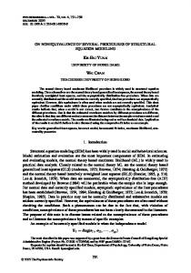
The first test ensures that the class k used by classifier A to label data has an accuracy at least as good as the accuracy of classifier B. The second test is to help prevent a degradation in performance of classifier B due to the increased noise in labels. The unlabeled examples that satisfy both criteria are la beled by classifier A for classifier B and vice versa. This process is repeated until no more unlabeled examples satisfy the criteria for either classifier. At the end of the co-training procedure (no unlabeled examples are labeled), the classifiers learned on the corresponding final labeled sets are evaluated on the test set. In our experiments we used two different classification algorithms – Naïve Bayes and C4.5 decision tree. We modified the C4.5 decision tree program to convert leaf frequencies into probabilities using the Laplace correction (Provost & Domingos, 2003). For the final prediction, the probability estimates from both Naïve Bayes and C4.5 are averaged. 2.2 ASSEMBLE The ASSEMBLE algorithm (Bennett et al., 2002) won the NIPS 2001 Unlabeled data competition. The intuition behind this algorithm is that one can build an ensemble that works consistently on the unlabeled data by maximizing the margin in function space of both the labeled and unlabeled data. To allow the same margin to be used for both labeled and unlabeled data, Bennett et al. introduce the concept of a pseudo-class. The pseudo-class of an unlabeled data point is defined as the predicted class by the ensemble for that point. One of the variations of the ASSEMBLE algorithm is based on AdaBoost (Freund & Schapire, 1996) that is adapted to the case of mixture of labeled and unlabeled data. We used the ASSEMBLE.AdaBoost algorithm as used by the authors for the NIPS Challenge. ASSEMBLE.AdaBoost starts the procedure by assigning pseudo-classes to the instances in the unlabeled set, which allows a supervised learning procedure and algorithm to be applied. The initial pseudo-classes can be assigned by using a 1-nearest-neighbor algorithm, ASSEMBLE-1NN, or simply assigning the majority class to each instance in the unlabeled datasets, ASSEMBLE-Class0. We treat majority class as class 0 and minority class as class 1 in all our datasets. The size of the training set over boosting iterations is the same as the size of the labeled set. Figure 1 shows the pseudo code of the ASSEMBLE.AdaBoost algorithm. In the pseudo code, L signifies the labeled set, U signifies the unlabeled set, l (size of the labeled set) is the sample size within each iteration and ß is the weight assigned to labeled or unlabeled data in the distribution D0 . The initial misclassification costs are biased towards the labeled data, due to more confidence in the labels. In the subsequent iterations of the algorithm, a, indicates the relative weight given to each type of error – either labeled data or unlabeled data error. In the pseudo-code, f indicates the supervised learning algorithm, which is Naïve Bayes for our experiments. T indicates the number of iterations, and f t (xi ) = 1 if an instance xi is correctly classified and f t (xi ) = -1, if it is incorrectly classified; ε is the error computed for each iteration t, and Dt is the sampling distribution. 336
Learning From Labeled And Unlabeled Data
1. l :=| L | and u :=| U | β / l 2. D1 ( i) := (1 − β ) / l
∀i ∈ L ∀i ∈U
3. yi := c, where c is the class of 1NN for i ∈ U or class 0 for i ∈ U, and original class for i ∈ L 4. f 1 = NaiveBayes (L + U) 5. for t := 1 to T do 6. Let yˆ i := f t (x i ), i = 1,..., L + U
7. ε = ∑ Dt [yi ≠ yˆ i], i = 1,..., L + U i
8. if ε > 0.5 then Stop 1 - ε 9. w t = 0.5 * log ε 10. Let Ft := Ft -1 + w t f t 11. Let y i = Ft (x i ) if i ∈ U 12. Dt +1 =
α i e − yi Ft +1 ( xi ) ∑ αi e
− yi Ft +1 ( xi )
∀i
i
13. S = Sample(L + U, Y, Dt + 1) 14. f t +1 = NaiveBayes (S) 15. end for 16. return Ft+1 Figure 1: ASSEMBLE.AdaBoost pseudo-code 2.3 Re-weighting Re-weighting (Crook & Banasik, 2002) is a popular and simple technique for reject-inferencing in credit scoring, but it has not been considered as a semi-supervised learning technique. It uses information on the examples from approved credit applications, i.e. labeled data, to infer conditional class probabilities for the rejected applications, i.e. unlabeled data. To apply re-weighting one assumes that the unlabeled data are MAR, i.e.
P(y = 1 | x,labeled = 1) = P(y = 1 | x,labeled = 0) = P(y = 1 | x) That is, at any x, the distribution of labeled cases having a y label is the same as the distribution of “missing” y (in the unlabeled population). There are several variants of re-weighting. According to the one we adopt here, also called extrapolation, the goal is first to estimate the distribution of classes for the la beled data within each 337
CHAWLA & KARAKOULAS
score group, and then extrapolate that distribution to the unlabeled data. Thus, a model is learned on the labeled training set and applied to the unlabeled data. The labeled and unlabeled data are grouped by score, i.e. posterior class probability from the model. The probabilities are percentile -binned, and each bin forms a score group. The unlabeled data are assigned labels based on the distribution of classes in corresponding score group from the labeled data. Thus, the key assumption is that the corresponding score-bands in the labeled and unlabeled data have the same distribution for the classes. This can be formulated as:
P( y k | S j , X L ) = P( yk | S j , X U ) ∴ y kjL / X Lj = y Ukj / X Uj where S j is the score band of group j, y kjL is the number of labeled examples belonging t o class yk in group j, and y U kj is the proportion of unlabeled examples that could be class y k in the score group j. The number of labeled cases in j are weighted by (|XLj +XUj |)/|XLj |, which is the probability sampling weight. To explain the re-weighting concept, let us consider the example given in Table 1. Let 0 and 1 be the two classes in the datasets. The score group of (0.6 - 0.7) is a bin on the posterior class probabilities of the model. The group weight for the example in Table 1 can be computed as (XL+XU )/XL = 1.2. Therefore, weighting the number of class0 and class1 in the group, we get class0 = 12; class1 = 108. Thus, we label at random 2 (=12-10) data points from the unlabeled set as class0, and 18 (=108-90) data points from the unlabeled set as class1. After labeling the unlabeled examples we learn a new model on the expanded training set (inclusive of both labeled and unlabeled data). Score Group 0.6 - 0.7
Unlabeled 20
Labeled
Class 0
Class 1
100
10
90
Table 1: Re-weighting example
2.4 Common Components Using EM The idea behind this technique is to eliminate the bias in the estimation of a generative model from labeled/unlabeled data of the MAR type. The reason for this bias is that in the case of such data the distributions of x given y in the labeled and unlabeled sets are different. We can remove this bias by estimating the generative model from both labeled and unlabeled data by modeling the missing labels through a hidden variable within the mixture model framework. In particular, suppose that the data was generated by M components (clusters), and that these components can be well modeled by the densities p ( x | j ,θ j ) , j = 1,2,..., M , with θ j denoting the corresponding parameter vector. The feature vectors are then generated according to the density: M
p ( x | θ ) = ∑ π j p ( x | j ,θ j ) j =1
338
Learning From Labeled And Unlabeled Data
where π j ≡ p( j ) are the mixing proportions that have to sum to one. The joint data log-likelihood that incorporates both labeled and unlabeled data takes the form:
L( Θ ) =
M
∑
( xi , yi )∈ X l
log ∑ π j p( xi | j ,θ j ) p ( yi | xi , j , ξ j ) + j =1
∑
xi ∈X u
M
log ∑ π j p ( xi | j , θ j ) j =1
Note that the likelihood function contains a "supervised" term, which is derived from X l labeled data, and an "unsupervised" term, which is based on X u unlabeled data. Consider applying the following simplistic assumption: the posterior probability of the class label is conditionally independent of the feature vector given the mixture component, i.e. p ( y i | xi , j , ξ j ) = p( yi | j ) . This type of model makes the assumption that the class conditional densities are a function of a common component (CC) mixture (Ghahramani & Jordan, 1994; Miller & Uyar, 1997). In general, we are interested in applying the CC mixture model to solve a classification problem. Therefore we need to compute the posterior probability of the class label given the observation feature vector. This posterior takes the form:
p ( y i | xi , Θ) =
M
∑ p ( j | xi , Θ) p ( y i | xi , j, ξ j ) = j =1
π p( x | j , θ ) j i j p( y i | j ) ∑ M π p ( x | l , θ ) j =1 ∑l =1 l i l M
One could also consider applying a separate component (SC) mixture model, where each class conditional density is modeled by its own mixture components. This model was essentially presented by Nigam et al. (2000) for the case of labeled/unlabeled data in document classification. All of these models, as well as more powerful ones that condition on the input feature vector, can be united under the mixture-of-experts framework (Jacobs et al., 1991). The application of this framework to the semi-supervised setting is further studied by Karakoulas and Salakhutdinov (2003).
2.4.1 Model Training Assume that p ( x | j ,θ j ) is parameterized by a Gaussian mixture component distribution for continuous data. We define the parameter vector for each component, j, to be θ j = ( µ j , Σ j ) for j = 1, 2,..., M ; where µ j is the mean, and Σ j is the covariance matrix of the jth component. In all of our experiments we constrain the covariance matrix to be diagonal. We also have two more model parameters that have to be estimated: the mixing proportion of the components, π j = p ( j ) , and β y | j = p ( y i | j ) the posterior class probability. i According to the general mixture model assumptions, there is a hidden variable directly related to how the data are generated from the M mixture components. Due to the labeled/unlabeled nature of the data, there is an additional hidden variable for the missing class labels of the unlabeled data. These hidden variables are introduced into the above log-likelihood L(Θ) . A general method for maximum likelihood estimation of the model parameters in the presence of hidden variables is the Expectation-Maximization (EM) algorithm (Dempster et al., 1977). The EM algorithm alternates between estimating expectations for the hidden variables (incomplete data) given the current model parameters and refitting the model parameters given the estimated, complete data. We now derive fixed-point EM iterations for updating the model parameters. 339
CHAWLA & KARAKOULAS
For each mixture component, j, and each feature vector, i, we compute the expected responsibility of that component via one of the following two equations, depending on whether the ith vector belongs to the labeled or unlabeled set (E-Step):
π tj β yi | j p( xi | j , θ tj )
p ( j | xi , yi , θ ) = t
M
∑ π lt β y |l p (x i | l ,θ lt ) i
l =1
p ( j | xi , θ ) = t
π tj p ( x i | j , θ tj ) M
∑ l =1
π lt
xi ∈ X L
xi ∈ X U
p ( x i | l ,θ lt )
Given the above equations the solution for the model parameters takes the form (M-Step):
1 t t p ( j | x , y , θ ) + p ( j | x , θ ) ∑ ∑ i i i N ( x , y )∈X xi ∈X u i i l
π tj+1 =
t +1 k| j
βy
∑ p ( j | xi , y i , θ t )
=
xi ∈ X l ∩ y i = k
∑ p ( j | x i , y i ,θ t )
( xi , yi )∈X l
µ tj +1 =
t t p ( j | x , y , θ ) x + p ( j | x , θ ) x ∑ ∑ i i i i i t +1 Nπ j ( xi , yi )∈X l xi ∈ X u
Σ tj+1 =
t t t t p ( j | x , y , θ ) S + p ( j | x , θ ) S ∑ ∑ i i ij i ij Nπ tj+1 ( xi , yi )∈X l xi ∈ X u
1
1
where we define N =| X l | + | X u | , and Sij ≡ ( xi − µ j )( xi − µ j ) . t
t T
Iterating through the E-step and M-step guarantees an increase in the likelihood function. For discrete-valued data, instead of using a mixture of Gaussians, we apply a mixture of multinomials (Kontkanen et al., 1996). In general, the number of components can be tuned via cross-validation. However, the large number of experiments reported in this work makes the application of such tuning across all experiments impractical, because of the computational overhead it would entail. Furthermore, the purpose of this paper is to provide insight into learning from labeled and unlabeled data with different techniques, rather than to find out which technique performs the best. For this reason we report the results from experiments using two, six, twelve and twenty-four components. We further 340
Learning From Labeled And Unlabeled Data
discuss this point in Section 4.
3. Dealing With Sample Selection Bias If there is a censoring mechanism that rules the assignment of a label to instances in the data then a model learned on only the labeled data will have a sample selection bias. In this case the decision for labeling can be due to unobserved features that create a dependency between assigning a label and the class label itself. Thus the data are of MNAR type. For example, suppose we are interested in assigning relevance to a text corpus, e.g., web pages, and that someone has subjectively decided which documents to label. The estimates for probability of relevance can then be underestimated, as the training set might not be representative of the complete population. This can result in an increase in the estimation bias of the model, thus increasing the error. We present two techniques, previously proposed in the literature, for dealing with MNAR data. 3.1 Bivariate Probit Heckman (1979) first studied the sample -selection bias for modeling labor supply in the field of Econometrics. Heckman's sample selection model in its canonical form consists of a linear regression model and a binary probit selection model. A probit model is a variant of a regression model such that the latent variable is normally distributed. Heckman's method is a two-step estimation process, where the probit model is the selection equation and the regression model is the observation equation. The selection equation represents the parameters for classification between labeled or unlabeled data – namely its purpose is to explicitly model the censoring mechanism and correct for the bias – while the observation equation represents the actual values (to regress on) in the labeled data. The regression model is computed only for the cases that satisfy the selection equation and have therefore been observed. Based on the probit parameters that correct for the selection bias, a linear regression model is developed only for the labeled cases. The following equations present the regression and probit models. The probit model is estimated for y2 . The dependent variable y2 represents whether data is labeled or not; y2 = 1 then data is labeled, y2 = 0 then data is unlabeled. The equation for y1 , the variable of interest, is the regression equation. The dependent variable y1 is the known label or value for the labeled data. The latent variables u 1 and u 2 are assumed to be bivariate and normally distributed with correlation ρ. This is the observation equation for all the selected cases (the cases that satisfy y2 >0). Let us denote by y1 * the observed values of y1 . Then we have:
y1 = β ' x1 + u1 y 2 = γ ' x 2 + u2 2
u1 , u2 ≈ N [ 0,0, σ u1 , ρ ] y1 = y1* , if y 2
>0
y1 ≡ missing if y2 ≤ 0 The estimate of β will be unbiased if the latent variables u 1 and u2 are uncorrelated, but that is 341
CHAWLA & KARAKOULAS
not the case as the data are MNAR. Not taking this into account can bias the results. The bias in regression depends on the sign of ρ (biased upwards if ρ is positive, and downwards if ρ is negative). The amount of bias depends on the magnitude of ρ and σ. The crux of Heckman’s method is to estimate the conditional expectation of u 1 given u 2 and use it as an additional variable in the regression equation for y1 . Let us denote the univariate normal density and CDF of u 1 by φ and Φ , respectively. Then,
E[ y1* | x1 , y 2 > 0] = β ' x1 + ρσ u λ 1 φ ( x2 γ ' ) where λ = Φ( x2 γ ' ) λ is also called the Inverse Mills Ratio (IMR), and can be calculated from the parameter estimates. Heckman's canonical form requires that one of the models be regression based. However, in this paper we deal with semi-supervised classification problems. For such problems a class is assigned to the labeled data, y1 = 0 or 1, only if y2 = 1. Given the two equations in Heckman’s method, the labeled data are only observed for y2 = 1. Thus, we are interested in E[y1 |x, y 2 = 1] or P(y1 |x, y 2 = 1). For example, to predict whether someone will default on a loan (bad customer), a model needs to be learnt from the accepted cases. Thus, in such scenarios one can use the bivariate probit model for two outcomes, default and accept (Crook & Banasik, 2002; Greene, 1998). The bivariate probit model can be written as follows:
y1 = β ′x1 +u1 y 2 = β ′x 2 +u 2 y1 = y1* for y 2 = 1 Cov(u1 , u 2 ) = ρ If ρ = 0 then there is no sample -selection bias associated with the datasets, that is the latent variables are not correlated and using the single probit model is sufficient. The log-likelihood of the bivariate model can be written as (where Φ 2 is the bivariate normal CDF and Φ is the univariate normal CDF).
Log ( L ) = ∑ y
2 =1, y1 =1
log F 2 [ β1 x1 , β 2 x 2 , ρ ]
+∑ y
2 =1, y1 =1
log F 2 [ −β1 x 1 , β 2 x 2 ,− ρ ]
− ∑ y 2=0 log F [ −β 2 x 2 ] We apply the bivariate probit model in the semi-supervised learning framework by introducing a selection bias in various datasets. 3.2 Sample -Select Zadrozny and Elkan (2000) applied a sample -selection model to the KDDCup-98 donors' dataset to assign mailing costs to potential donors. There is sample sele ction bias when one tries to predict the donation amount from only donors’ data. Using Naïve Bayes or the probabilistic version of C4.5, 342
Learning From Labeled And Unlabeled Data
they computed probabilistic estimates for membership of a person in the ''donate'' or ''not donate'' category, i.e. P(labeled=1|x). They then imputed the membership probability as an additional feature for a linear regression model that predicts the amount of donation. Zadrozny and Elkan did not cast the above problem as a semi-supervised learning one. We adapted their method for the semi-supervised classification setting as follows:
= P( labeled = 1 | x, L ∪ U ) n +1 ∴ P( y = 1 |x ∪ x , L) n +1 x
L is the labeled training set, U is the unlabeled set, labeled=1 denotes an instance being labeled, labeled = 0 denotes an instance being unlabeled, and y is the label assigned to an instance in the labeled set. A new training set of labeled and unlabeled datasets (L∪ U ) is constructed, wherein a class label of 1 is assigned to labeled data and a class label of 0 is assigned to unlabeled data. Thus, a probabilistic mode l is learned to classify data as labeled and unlabeled data. The probabilities, P(labeled = 1|x), assigned to labeled data are then included as another feature in the labeled data only. Then, a classifier is learned on the modified labeled data (with the additional feature). This classifier learns on "actual" labels existing in the labeled data. For our experiments, we learn a Naïve Bayes classifier on L∪ U, and then impute the posterior probabilities as another feature of L, and relearn the Naïve Bayes classifier from L. For the rest of the paper we will call this method Sample-Select. While we apply the Sample -Select method along with other semi-supervised techniques, we only apply the bivariate probit model to the datasets particularly constructed with the sample-selection bias. This is because Sample -Select is more appropriate for the MAR case rather than the MNAR case due to the limiting assumption it makes. More specifically, in the MNAR case we have P(labeled,y|x,ξ,ω)=P(y|x,labeled,ξ)*P(labeled|x,ω) However, since Sample -Select assumes P(y|x,labeled=0,ξ)= P(y|x,labeled=1,ξ) this reduces the problem to MAR.
4. Experimental Set-up The goal of our experiments is to investigate the following questions using the aforementioned techniques on a variety of datasets: (i) (ii) (iii) (iv) (v)
What is the effect of independence or dependence among features? How much of unlabeled vs. labeled data can help? What is the effect of label noise on semi-supervised techniques? What is the effect of sample -selection bias on semi-supervised techniques? Does semi-supervised learning always provide an improvement over supervised learning?
For each of these questions we designed a series of experiments real-world and artificial 343
CHAWLA & KARAKOULAS
datasets. The latter datasets were used for providing insights on the effects of unlabeled data within a controlled experimental framework. Since most of the datasets did not come with a fixed labeled/unlabeled split, we randomly divided them into ten such splits and built ten models for each technique. We reported results on the average performance over the ten models for each technique. Details for this splitting are given in Section 4.1. Each of the datasets came with a pre-defined test set. We used those test sets to evaluate performance of each model. The definition of the AUC performance measure is given in Section 4.2. As mentioned earlier, the purpose of this work is to provide insight into learning from labeled and unlabeled data with different techniques, rather than to find out which technique performs the best. The latter would have required fine-tuning of each technique. However, to understand the sensitivity of the various techniques with respect to key parameters, we run experiments with different parameter settings. Thus, for the common-component technique, we tried 2, 6, 12, and 24 components; for ASSEMBLE-1NN and ASSEMBLE-Class0 we tried 0.4, 0.7 and 1.0 as values for α, the parameter that controls the misclassification cost; for co-training we tried 90%, 95% and 99% confidence intervals for deciding when to label. Appendix A (Tables 6 to 9) presents the results for these four techniques, respectively. The common-component technique with 6 components gave consistently good performance across all datasets. We found marginal or no difference in the performance of co-training for different confidence intervals. We found small sensitivity to the value of a at lower amounts of labeled data, but as the labeled data increases the differences between the values of a for various datasets becomes smaller. Moreover, not all datasets exhibited sensitivity to the value of a. Our observations agree with Bennett et al. (2002) that choice of a might not be critical in the cost function. Thus, for analyzing the above questions we set the parameters of the techniques as follows: 6 components for common-component mixture, α = 1 for ASSEMBLE-1NN and ASSEMBLE-Class0, and confidence of 95% for co-training. 4.1 Datasets We evaluated the methods discussed in Sections 2 and 3 on various datasets, artificial and real-world, in order to answer the above questions. Table 2 summarizes our datasets. All our datasets have binary classes and are unbalanced in their class distributions. This feature makes the datasets relevant to most of the real-world applications as well as more difficult for the semi-supervised techniques, since these techniques can have an inductive bias towards the majority class. To study the effects of feature relevance and noise we constructed 5 artificial datasets with different feature characteristics and presence of noise. We modified the artificial data generation code provided by Isabelle Guyon for the NIPS 2001 Workshop on Variable and Feature Selection (Guyon, 2001). The convention used for the datasets is: A_B_C_D, where § A indicates the percentage of independent features, § B indicates the percentage of relevant independent features, § C indicates the percentage of noise in the datasets, and § D indicates the percentage of the positive (or minority) class in the datasets. The independent features in the artificial datasets are drawn by N(0,1). Random noise is added 344
Learning From Labeled And Unlabeled Data
to all the features by N(0,0.1). The features are then rescaled and shifted randomly. The relevant features are centered and rescaled to a standard deviation of 1. The class labels are then assigned according to a linear classification from a random weight vector, drawn from N(0,1), using only the useful features, centered about their mean. The mislabeling noise, if specified, is added by randomly changing the labels in the datasets. The naming of the artificial datasets in Table 2 are self-explanatory using the convention outlined earlier. Datasets
Training Size |L+U|
Testing Size
Class-distribution (majority:minority)
Features
30_30_00_05
8000
4000
95:5
30
30_80_00_05
8000
4000
95:5
30
80_30_00_05
8000
4000
95:5
30
80_80_00_05
8000
4000
95:5
30
30_80_05_05
8000
4000
95:5
30
30_80_10_05
8000
4000
95:5
30
30_80_20_05
8000
4000
95:5
30
SATIMAGE (UCI)
4435
2000
90.64:9.36
36
WAVEFORM (UCI)
3330
1666
67:33
21
ADULT (UCI)
32560
16281
76:24
14
2710
71.7:28.3
12
800
61.75:38.25
25
0.6:99.4
200
NEURON (NIPS)
L
530 + 2130 U
HORSE-SHOE (NIPS)
400 L + 400 U
KDDCUP-98 (UCI)
4843 L +
96367
90569 U Table 2: Datasets details
Three of our real-world datasets – waveform, satimage, and adult – are from the UCI repository (Blake et al., 1999). We transformed the original six-class satimage datasets into a binary class problem by taking class 4 as the goal class (y=1), since it is the least prevalent one (9.73%), and merging the remaining classes into a single one. Two of the datasets come from the NIPS 2001 (Kremer & Stacey, 2001) competition for semi-supervised learning with pre-defined labeled/unlabeled subsets. We randomly divided ten times all the above artificial and UCI datasets into five different labeled-unlabeled partitions: (1,99)%, (10,90)%, (33,67)%, (67,33)%, (90,10)%. This provided us with a diverse test bed of varying labeled and unlabeled amounts. We report the results averaged 345
CHAWLA & KARAKOULAS
over the ten random runs. The last real-world dataset is from the KDDCup-98 Cup (Heittich & Bay, 1999; Zadrozny & Elkan, 2000). This is a typical case of sample selection bias, i.e. MNAR. We converted the original KDDCup-98 donors regression problem into a classification problem so that is consistent with the semi-supervised classification setting of the experiments. We considered all the respondents to the donation mailing campaign as the labeled set and the non-respondents as the unlabeled set. We then transformed the labeled set into a classification problem, by assigning a label of “1” to all the individuals that make a donation of greater than $2, and a label of “0” to all the individuals that make a donation of less than $2. This gave us a very difficult dataset since due to the sample selection bias built into the dataset the labeled and unlabeled sets had markedly different class distributions. The positive class in the training set is 99.5%, while in the testing set it is only 5%. We also created a biased version of the Adult dataset and the (30_80_00_05) artificial dataset with MAR labels in order to study the effect of this missing label mechanism on the techniques. More specifically, for the biased Adult dataset we constructed the labeled and unlabeled partitions of the training set by conditioning on the education of an individual. Using this censoring mechanism all the individuals without any post high-school education were put into the unlabeled set, and the rest into the labeled set. Thus, we converted the original classification problem into a problem of return of wages from adults with post high-school education. For the (30_80_00_05) dataset we divided it into labeled and unlabeled sets by conditioning on two features such that: if (xin


![columbus - Notre Dame Campus Tour - University of Notre Dame [PDF]](https://m.moam.info/img/260x300/columbus-notre-dame-campus-tour-university-of-notr_6479c497098a9ef8668b4658.jpg)